A useful place to begin is with the central tension in self-supervised vision: we want an encoder to learn from images without labels, but we do not want the pretraining task itself to quietly define the wrong notion of “understanding.” If the learned representation is later frozen and used for downstream tasks, then the pretraining signal has to encourage features that are semantic enough to transfer: object identity for classification, approximate numerosity for counting, geometry for depth, and many other properties that were never explicitly annotated during training.

Formally, we start with unlabeled images $I$ and train an encoder, often a Vision Transformer $f_\theta$, to produce representations that will later be reused. After pretraining, the encoder is commonly frozen, and a lightweight task-specific head is trained on top. This is why linear evaluation accuracy, often reported as $\mathrm{Top1}$, is such a useful diagnostic: if a linear classifier can extract category information from frozen features, then the representation already organizes images in a semantically meaningful way.

But the hard question is: what self-supervised prediction problem should force those semantics to emerge? Two dominant families of methods answer this differently. Joint-embedding methods often create two transformed “views” of the same image and train the model to make their representations agree. Masked image modeling methods often hide patches and ask the model to reconstruct missing pixels. Both strategies have been enormously influential, but both come with a possible mismatch between the pretraining objective and the representations we ultimately want.

The first risk is that hand-crafted view augmentations bake in assumptions. If we train a model to be invariant to random crops, color jitter, blur, or solarization, we are implicitly declaring that these transformations should not change semantic meaning. Often that is helpful. But it is not universally true. Cropping can remove the object of interest; color may matter for fine-grained recognition; geometric transformations may interfere with localization or depth. In other words, the augmentations are not neutral—they encode task-biased invariances.

The second risk is that pixel reconstruction can overemphasize low-level detail. If a model is rewarded for reconstructing RGB values, it may spend substantial capacity modeling texture, color continuity, and local statistics. Those details are real information, but they are not always the information we want a frozen encoder to prioritize. A pixel-level objective can succeed by becoming good at plausible image completion while still failing to build representations that are maximally useful for semantic transfer.

I-JEPA, the Image-based Joint-Embedding Predictive Architecture, takes a different route. Its claim is deceptively simple: predict missing information in representation space, not in pixel space, and do so without relying on pairs of hand-crafted augmented views. Instead of asking the model to reproduce the raw pixels of a hidden region, I-JEPA asks it to predict the representation that another encoder would assign to that region. The target is not “what exact colors go here?” but rather “what abstract representation should this missing part have, given the visible context?”

At a high level, we choose a visible context $x$ from an image $I$, with $x \subset I$. The context is encoded into a representation $s_x$. For a missing target block indexed by $i$, a predictor $g_\phi$ receives the context representation and information about the masked positions, represented by mask tokens $\{m_j : j \in B_i\}$. It then predicts a target representation:

$$x \subset I,\qquad \hat{s}_y(i)=g_\phi\bigl(s_x,\{m_j:j\in B_i\}\bigr), \qquad \hat{s}_y(i)\approx s_y(i).$$

The important phrase is $\hat{s}_y(i)\approx s_y(i)$. The model is not trained to make $\hat{y}$ look like a missing patch in RGB space. It is trained to make the predicted embedding $\hat{s}_y(i)$ match the target embedding $s_y(i)$. This places the learning signal at a more abstract level. If the target encoder produces semantic features, then the context encoder and predictor are pressured to infer semantic content from surrounding evidence.

This objective also changes what “prediction” means. Predicting pixels often rewards local realism: edges line up, colors continue, textures match. Predicting representations rewards compatibility with a learned feature space. That makes the task less about filling in every visual detail and more about inferring the latent structure that explains the image. The hope is that, by avoiding both augmentation-defined invariances and raw pixel reconstruction, the learned encoder becomes broadly useful rather than specialized to a pretext task’s quirks.

There are still subtle assumptions. I-JEPA assumes that the target representations are themselves meaningful enough to serve as learning signals, and that the masking strategy forces nontrivial contextual reasoning rather than shortcut prediction. If the hidden regions are too small or too locally predictable, the model may learn shallow continuity. If they are too large or disconnected from the context, prediction may become ambiguous. The design therefore depends on masking blocks at a scale where the model must use semantic context, not merely interpolate textures.

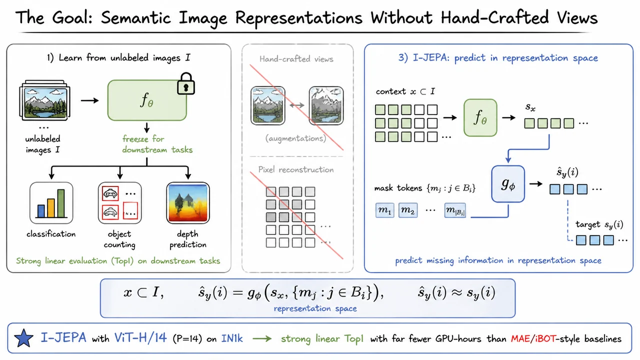
The visual summary below condenses this motivation into three pieces. On the left is the practical goal: train on unlabeled images, freeze the encoder, and transfer the representation to downstream tasks such as classification, counting, and depth prediction. In the middle are the two routes I-JEPA is trying to avoid as primary supervision signals: hand-crafted augmented views and pixel-level reconstruction.

On the right is the core alternative: use visible context $x$, encode it as $s_x$, combine it with mask-position information, and predict the missing block’s representation $\hat{s}_y(i)$ so that it matches $s_y(i)$. The headline empirical motivation is that this kind of representation-space prediction can scale to large ViTs—for example ViT-H/14 with patch size $P=14$ trained on $\mathrm{IN1k}$—while producing strong frozen-feature linear $\mathrm{Top1}$ performance with substantially less compute than several MAE- or iBOT-style baselines.

The previous point sets a high bar: we do not merely want features that make ImageNet linear probes happy; we want semantic image representations that remain useful when the downstream task changes. That is exactly where a first failure mode of popular view-invariance methods appears. Their success comes from making two transformed views of the same image agree, but the choice of transformations quietly defines what the model is allowed to forget.

In a typical joint-embedding method such as SimCLR, BYOL, DINO-style training, or related contrastive/non-contrastive approaches, we begin with an image $I$, sample two augmentations $t_1$ and $t_2$, and train an encoder so that

$$f(t_1(I)) \approx f(t_2(I)).$$

The objective is not literally saying “understand the whole image.” It is saying something more specific: produce similar representations after these hand-chosen perturbations. If the perturbations are semantically harmless, this is a powerful idea. A dog remains a dog under a crop, a color jitter, a blur, or a resize. For classification, these invariances are often exactly what we want.

But the hidden assumption is stronger than it first appears: whatever the augmentation removes or corrupts must be irrelevant to the representation. If a random crop cuts out half the scene, the model is still encouraged to map the crop close to another view of the original image. If color jitter removes appearance information, the representation is discouraged from depending too much on color. If blur destroys texture, or resizing changes apparent scale, the model is pushed toward features that survive those changes.

That pressure is not automatically wrong. In fact, it explains why view-invariance methods have been so effective for object category recognition. Classification often benefits from discarding nuisance variation:

• exact object position,
• background clutter,
• lighting and color shifts,
• small texture details,
• moderate changes in scale.

For a classifier, these details may be distractions. A robust “dogness” representation should not change much because the image was slightly blurred or the colors were altered.

The problem is that classification is only one downstream task. Many vision problems require precisely the information that standard augmentations treat as disposable. For object counting, a crop may remove one instance and change the correct answer. For depth estimation, resizing and cropping can distort cues about scale, perspective, and spatial relationships. For segmentation, weakening spatial layout is especially dangerous: the model must know not only what is present, but where each region and boundary lies. Color may also matter for materials, biological images, medical images, remote sensing, and fine-grained recognition.

So the issue is not simply “augmentations are bad.” The issue is that augmentations encode a task-biased invariance prior. They tell the representation which factors of variation should be ignored before we know which downstream task we care about. This is acceptable if the pretraining goal is aligned with classification-like transfer, but it becomes limiting when we want a more general visual representation.

This motivates one of I-JEPA’s central design choices: avoid relying on hand-crafted view augmentations as the main source of supervision. Instead of forcing agreement between aggressively transformed views, I-JEPA asks the model to predict missing information from visible context—but crucially, it predicts that information in representation space, not pixel space. The hope is to preserve semantic structure without requiring the designer to specify, through augmentations, which visual information should be invariant.

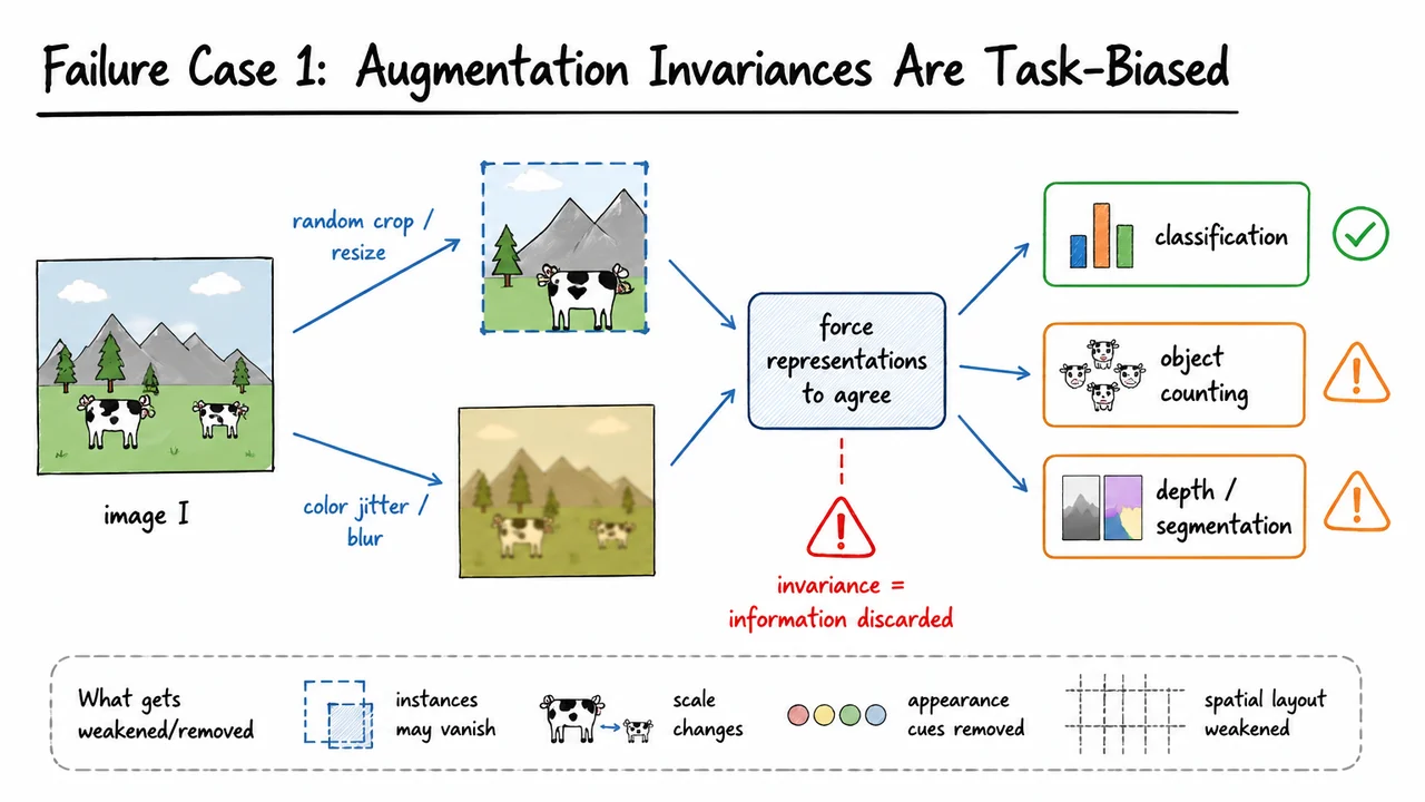
The visual below compresses this failure mode into a single causal chain. An image is transformed into multiple views through operations such as cropping, resizing, color jitter, and blur. The learning rule then forces the resulting representations to agree. That agreement is useful for classification, where invariance is often beneficial, but it can become harmful for tasks that depend on instance count, scale, appearance, or spatial layout.

The key takeaway is the warning in the middle: invariance means information has been discarded. Sometimes that discarded information is nuisance variation; sometimes it is the signal required by the next task. I-JEPA starts from this observation and asks whether self-supervised learning can avoid baking in so many manually chosen invariances while still learning high-level, transferable representations.

Avoiding hand-crafted augmentations removes one source of bias, but it does not automatically make the learning problem unbiased. A different family of self-supervised methods avoids explicit view design by corrupting the image itself and asking the model to fill in what is missing. This is the intuition behind masked image modeling: instead of saying “these two augmented views should match,” we say “given the visible part of the image, predict the hidden part.”

Formally, we start from an image signal $y$, then construct a corrupted or masked context $x$:

$$x = \text{masked or corrupted view of } y.$$

The model observes $x$, not the full image, and is trained to recover the missing content of $y$. In MAE-style methods, for example, a large fraction of image patches is removed, the encoder processes the visible patches, and a decoder reconstructs the missing pixels or patch-level visual tokens. This is attractive because it uses the image itself as supervision: no labels, no manually chosen positive pairs, no explicit color jitter or cropping policy that encodes assumptions about invariance.

But the choice of prediction target matters just as much as the choice of input corruption. If the target is raw pixels, then the loss function rewards whatever helps reduce pixel-level error. A typical reconstruction objective has the form

$$\mathcal{L}_{\text{pixel}} = \left\| \hat{y}_{\text{masked}} - y_{\text{masked}} \right\|^2,$$

or some variant defined over pixels, patches, or low-level visual tokens. This objective is perfectly sensible if the goal is image reconstruction. However, if the goal is semantic representation learning, it can overemphasize details that are only weakly connected to meaning.

The failure mode is subtle: the model is not “wrong” to learn texture, color, edges, and local continuity. Those cues are genuinely useful for reconstructing an image. If a missing patch contains grass, sky, fur, fabric, or a brick wall, then local statistics can be highly predictive. The model can improve its loss by becoming very good at short-range visual interpolation: matching colors, extending contours, reproducing texture frequencies, and respecting local patch boundaries.

The problem is that these are not always the features we want a frozen representation to prioritize. Many downstream tasks care more about objects, spatial layout, parts, relations, and category-level abstraction than about exact RGB values. A representation that preserves fine texture beautifully may still be less linearly organized by semantic class. This helps explain a common empirical pattern: masked autoencoder-style reconstruction can scale well and fine-tune very effectively, but its frozen features are often less semantic under linear probing or limited-label transfer than methods whose objectives more directly shape the representation space.

This does not mean pixel reconstruction is bad. It is useful, stable, and often very scalable. The issue is one of optimization pressure. When the loss is computed in pixel space, every low-level discrepancy is visible to the objective, while many high-level semantic equivalences are not. Two patches may differ substantially in pixels but play the same semantic role; conversely, two textures may be locally predictable while saying little about object identity. The reconstruction objective has no inherent reason to prefer the abstraction unless the architecture, data scale, or downstream fine-tuning later forces it to.

I-JEPA’s response is to keep the appealing part of masked prediction—learning from missing information in an image—while changing the target of prediction. Instead of predicting raw pixels, I-JEPA predicts abstract representation targets. The model is asked to infer the representation of a hidden region from the representation of a visible context. This shifts the learning problem away from “what exact colors and textures were missing?” toward “what high-level information about the scene is implied by the visible content?”

A useful way to summarize the contrast is:

• Pixel reconstruction asks for low-level fidelity.
• Representation prediction asks for agreement in an abstract embedding space.
• The motivation for I-JEPA is that semantic structure should be learned before the model is rewarded for rendering detail.

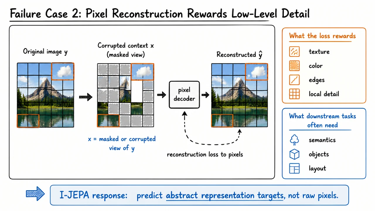
The visual below condenses this motivation into a compact comparison. On the left, masked image modeling begins with a full image signal $y$, produces a corrupted context $x$, and trains a pixel decoder to reconstruct the missing content. The highlighted patches emphasize the kinds of local evidence that a pixel-space loss naturally rewards: color, texture, edges, and nearby continuity.

On the right, the callouts separate what the reconstruction loss directly optimizes from what downstream recognition tasks often need. This is the key conceptual bridge into I-JEPA: rather than spending the pretraining objective on raw visual detail, predict targets in a representation space where the desired abstractions—objects, layout, and semantic context—can become the central currency of learning.

If pixel reconstruction pulls a model toward texture, edges, and color statistics, the natural question is: what kind of prediction target would force the model to understand the image without asking it to reproduce the image? This is the core motivation behind I-JEPA. It tries to occupy a middle ground between two familiar self-supervised extremes: learning invariances through hand-designed augmentations, and learning local detail through generative reconstruction.

The first extreme is the classic joint-embedding strategy: take two transformed views of the same image, encode them, and train their representations to agree. This can be very effective, but the semantics learned by the model depend heavily on the augmentations we choose. If random crops, color jitter, blur, or solarization define what should be invariant, then the training pipeline is quietly injecting human assumptions about vision. Sometimes those assumptions are helpful; sometimes they erase information that matters. A crop-based objective may encourage object-level semantics, but it may also teach the model to ignore spatial layout, small objects, or context that is predictive but frequently removed.

The second extreme is masked image modeling with a pixel-space decoder. Here the task is often easy to specify: hide patches and reconstruct them. But as we just saw, a pixel-level target rewards any information useful for matching RGB values. That includes semantic structure, but it also includes low-level regularities: local texture continuation, lighting, chromatic smoothness, and edge interpolation. A sufficiently strong decoder can solve much of the task by modeling image statistics rather than learning representations that transfer well to recognition, localization, or reasoning.

I-JEPA’s insight is to change where prediction happens. Instead of predicting pixels, it predicts representations of missing image regions. A context encoder sees part of the image. A target encoder sees the held-out region. The predictor is trained to infer the target region’s embedding from the context embedding and information about where the target block is located. In words, the model is asked:

> Given the visible context, what should the representation of the missing region be?

That target is deliberately not a raw patch. It is a feature vector produced by another neural network. This matters because representation space can discard nuisance variation that pixel space preserves. If the target encoder maps two visually different but semantically similar patches to nearby vectors, then the predictor is not punished for failing to reproduce exact texture or color. The hope is that the training signal emphasizes semantic compatibility: objects, parts, spatial relations, and scene-level regularities.

This also explains why I-JEPA does not need the same kind of hand-crafted view augmentations as contrastive or Siamese joint-embedding methods. Instead of saying, “these two augmented views must match,” I-JEPA says, “this missing region should be predictable from this context in representation space.” The invariances are therefore not imposed primarily by color jitter or crop recipes; they emerge from the predictive structure of the task and from the abstraction level of the target representation.

There is an important subtlety here: I-JEPA is not claiming that prediction alone magically creates semantics. If the target representation were allowed to remain too close to pixels, the method could still overfit low-level detail. If the target representation collapsed to a constant vector, prediction would become trivial. And if the masked regions were too small or too local, the model might again solve the task with short-range texture cues. The design therefore depends on several interacting choices:

• Predict in embedding space, not RGB space.
• Use large target blocks, so prediction requires nontrivial context.
• Separate context and target encoders, so the target can provide a stable learning signal.
• Update the target encoder slowly, often with an exponential moving average, to avoid chasing a moving or degenerate target.

The result is a pretraining problem that is neither purely discriminative nor purely generative. It is predictive, but not reconstructive. It learns by filling in missing information, but the thing being filled in is an abstract representation rather than pixels. This is why I-JEPA is best understood as a joint-embedding predictive architecture: it combines the semantic bias of embedding-based learning with the structured signal of masked prediction.

The visual below condenses this design choice into a simple contrast. Pixel reconstruction asks the model to recover visible detail and therefore risks rewarding low-level accuracy. Augmentation-based joint embedding asks the model to agree across hand-crafted views and therefore inherits the assumptions built into those views. I-JEPA instead routes the learning signal through a representation target: context goes in, a missing-region embedding is predicted, and the comparison happens in feature space.

That compact picture is useful because it frames I-JEPA as a response to both failure cases at once. It avoids making pixels the final authority, while also avoiding the need to manually specify every invariance through augmentations. The next issue is that joint-embedding systems have their own danger: if the representation target is not controlled carefully, the model may find a trivial collapsed solution. That is where the architecture and training dynamics become essential.

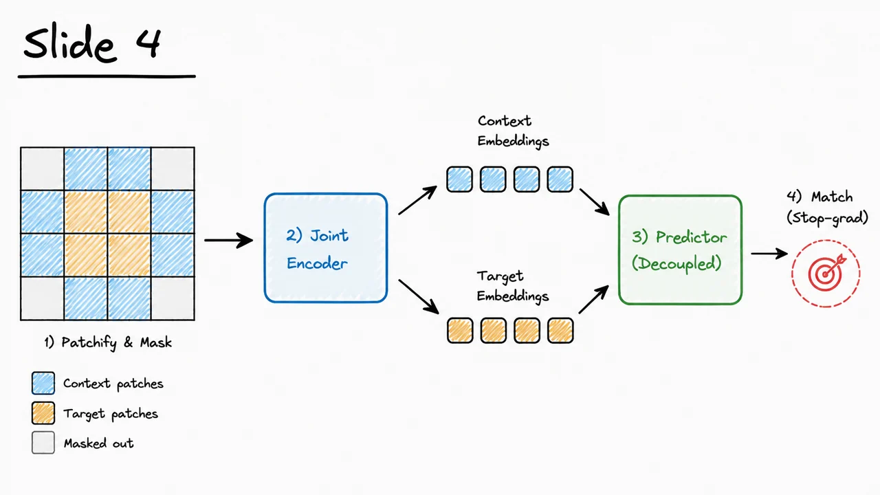
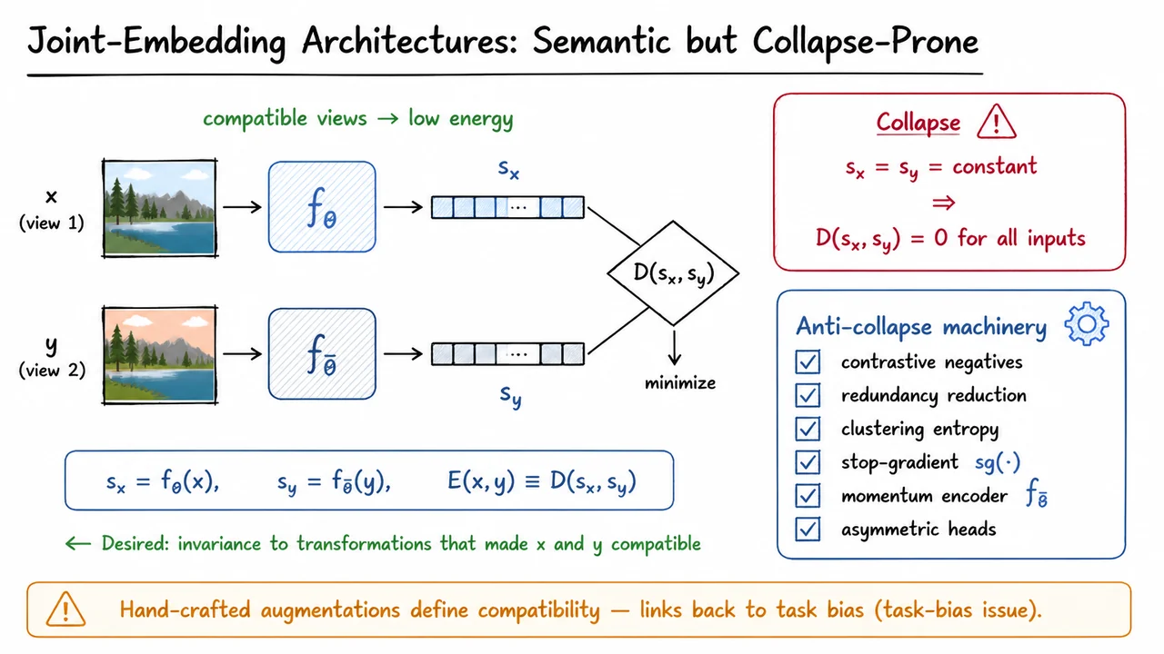
To understand why I-JEPA predicts in representation space rather than pixel space, it helps to first separate two families of self-supervised learning ideas. The first family is joint-embedding learning: take two related inputs, encode them, and train the encoders so that their representations agree. This is the conceptual lineage of methods such as Siamese networks, contrastive learning, BYOL, SimSiam, VICReg, Barlow Twins, SwAV, and related approaches.

The basic setup is simple. Suppose $x$ and $y$ are two compatible views of the same underlying content: perhaps two crops of the same image, or two differently augmented versions of it. A joint-embedding architecture maps each view into a representation space,

$$s_x=f_\theta(x),\qquad s_y=f_{\bar\theta}(y),$$

and assigns low energy when the two representations are close:

$$E(x,y)\equiv D(s_x,s_y).$$

Training then minimizes $D(s_x,s_y)$ for compatible pairs. The hope is that the model learns to ignore whatever changed between $x$ and $y$, while preserving what they share. If one view is color-jittered and the other is not, the model is encouraged to become invariant to color changes. If one view is a crop of the other, the model is encouraged to recognize the same object or scene despite partial observation.

This is why joint-embedding methods are often good at learning semantic invariances. They do not have to reconstruct every pixel. They only need to map related inputs to nearby points in representation space. That makes the learning signal less tied to low-level details such as texture, exact color, sensor noise, or background clutter. In a well-designed setup, the representation can focus on higher-level factors: object identity, scene layout, category-level structure, pose, or other stable semantic properties.

But the same elegance creates a serious failure mode: representational collapse. If the objective only says “make compatible representations close,” then the trivial solution is to map every input to the same vector. In that case,

$$s_x=s_y=\text{constant} \quad\Longrightarrow\quad D(s_x,s_y)=0\ \text{for all inputs}.$$

This solution perfectly minimizes the matching loss, but it contains no information about the image. Every dog, airplane, tree, and street scene receives the same representation. The energy is low everywhere, not because the model has understood compatibility, but because it has destroyed all distinctions.

The central challenge for joint-embedding learning is therefore not merely to make positive pairs close. It is to make them close without allowing all inputs to become identical. Different methods solve this problem in different ways:

• Contrastive methods use negative examples, pushing apart representations of different images.
• Redundancy-reduction methods penalize degenerate covariance or correlation structure across embedding dimensions.
• Clustering methods impose entropy or balanced-assignment constraints so that samples spread across prototypes.
• Stop-gradient and predictor asymmetry prevent both branches from chasing the same trivial solution too directly.
• Momentum encoders update one branch more slowly, creating a more stable target network.

These mechanisms are not incidental engineering tricks. They are what make joint-embedding objectives viable. Without some anti-collapse pressure, representation matching alone is underconstrained.

There is also a subtler issue: even if collapse is prevented, the notion of “compatible views” is usually defined by hand-crafted augmentations. We decide in advance that two random crops, color distortions, blur transformations, or solarized versions should be treated as equivalent. That injects a task bias into the learned representation. If the augmentations match the downstream semantics, the representation can be excellent. If they erase information that matters, or preserve nuisance factors that should be ignored, the learned invariances may be misaligned.

This is especially important for images. Cropping can teach object-level invariance, but it can also remove context or small objects. Color jitter can encourage robustness, but color may be semantically meaningful for some tasks. Strong augmentations can produce impressive transfer results, yet the pretext task is still partially designed by human assumptions about what should and should not matter.

So joint-embedding architectures give us a powerful lesson: prediction in representation space can emphasize semantics, because the model is not forced to reproduce pixels. But they also expose two limitations that I-JEPA wants to address. First, representation matching needs a way to avoid collapse. Second, when compatibility is defined by augmentations, the learned invariances inherit augmentation bias.

The visual below condenses this tradeoff. On the left, two compatible image views $x$ and $y$ pass through encoders and are encouraged to produce nearby embeddings $s_x$ and $s_y$, lowering the energy $D(s_x,s_y)$. That is the attractive part of joint embedding: it can learn invariance by matching representations rather than reconstructing images.

On the right, the collapse equation highlights the danger of an unconstrained matching objective. The anti-collapse checklist summarizes why practical joint-embedding systems require additional machinery. The bottom callout points to the motivation that will carry into I-JEPA: instead of relying entirely on hand-crafted view augmentations, can we define a predictive task in representation space that preserves the semantic benefits while reducing augmentation-driven task bias?

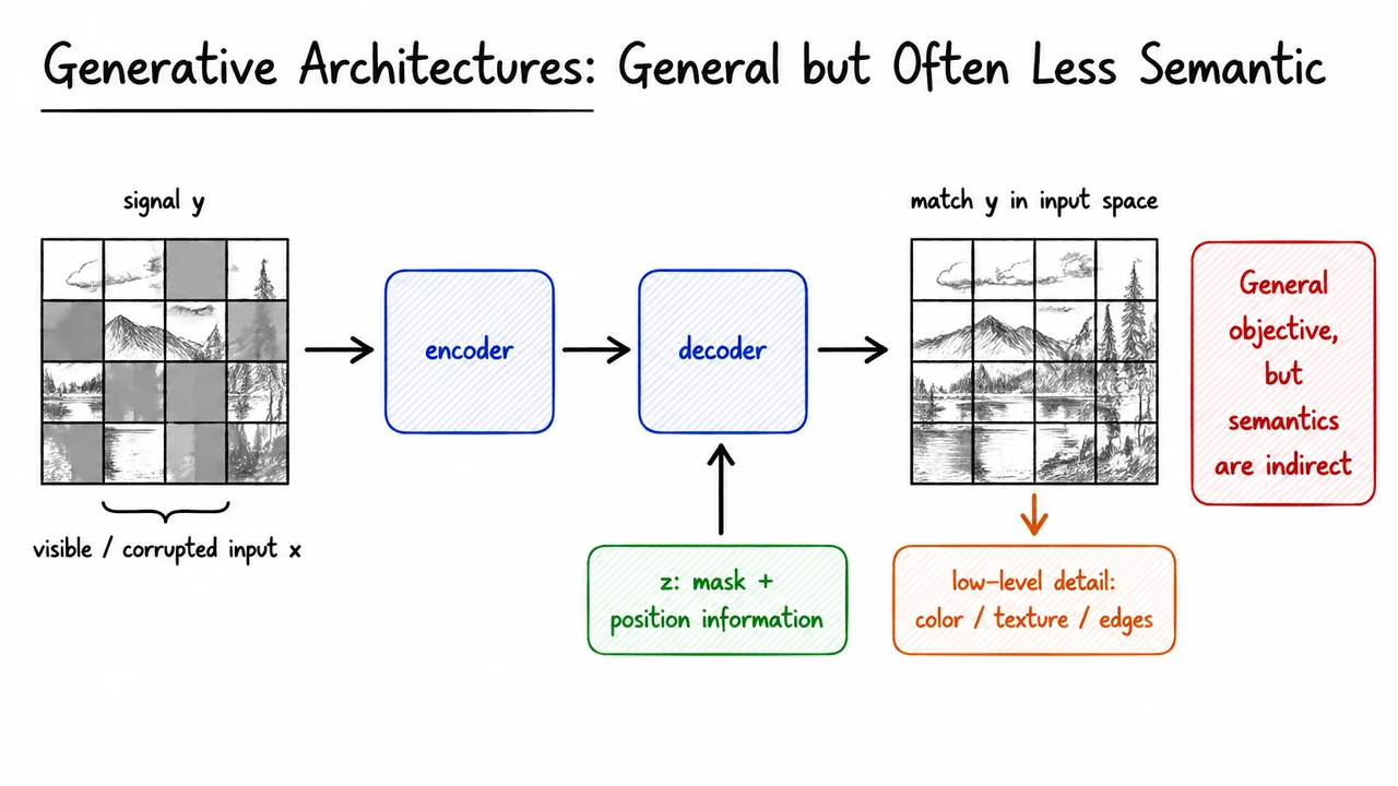
The previous discussion leaves us with an obvious temptation: if joint-embedding methods can collapse unless we carefully shape the objective, why not avoid that problem by asking the model to reconstruct the data itself? This is the central appeal of generative self-supervised learning. Instead of merely pulling two learned embeddings together, we corrupt or hide part of the input and train a model to recover the original signal. The target $y$ is no longer just another representation; it is the image, patch, token, or pixel signal itself.

From the energy-based viewpoint, a generative architecture makes $x$ compatible with $y$ by assigning low “energy” to reconstructions that match the observed data. Operationally, the pipeline is simple: take a visible or corrupted input $x$, encode it into a latent representation, decode that latent representation—often with additional conditioning information—and penalize the difference between the reconstruction and the target $y$ in input space.

In masked image modeling, for example, the model sees only some patches of an image. The missing patches must be inferred from the visible context. But the decoder is usually not asked to solve this problem from the latent representation alone. It also receives information such as:

• which patches are missing,
• where those patches belong,
• and sometimes explicit mask or position embeddings.

This conditioning variable, which we can loosely denote by $z$, tells the decoder the structure of the prediction problem. The encoder may summarize the visible content, while $z$ tells the decoder how to place predictions back into the image grid.

This setup has an important advantage over pure joint-embedding learning: collapse is much less natural. If the representation contains almost no information about the input, the decoder cannot simply output one constant image and achieve a good reconstruction loss across diverse targets. A constant output might minimize some trivial average error, but it will fail to match the many possible colors, shapes, textures, and object arrangements present in real images. In this sense, reconstruction gives the learning problem a built-in anti-collapse pressure.

That robustness is one reason generative SSL methods such as autoencoding and masked image modeling have been so influential. They define a broad, general-purpose objective: recover the data. This objective does not require hand-designed positive pairs, strong view augmentations, or a delicate balance of invariance and variance constraints. If the model can predict missing or corrupted parts of the signal, it must have learned something about the structure of the data distribution.

But this strength is also the source of a subtle weakness. A pixel-space or patch-space loss rewards everything that is predictable in the input, not only the information we would like a frozen representation to preserve for semantic transfer. The model may spend capacity modeling:

• local color continuity,
• texture statistics,
• edge sharpness,
• illumination patterns,
• patch-level correlations,
• and other low-level regularities.

These are real statistical structures, and they are useful for reconstruction. However, they are not necessarily the same structures needed for object recognition, scene understanding, or high-level visual reasoning. A representation can be excellent at supporting a decoder that fills in plausible pixels while still being less ideal as a frozen semantic feature.

This helps explain a recurring empirical pattern in self-supervised vision: strong reconstruction does not automatically imply strong semantics. A model may produce visually convincing completions or achieve a low reconstruction loss, yet its intermediate representations may transfer less well to classification or other semantic tasks than representations learned by contrastive or joint-embedding methods. The objective is not wrong; it is just aimed at a broader target. It asks the model to preserve enough information to regenerate the signal, and the signal contains far more than semantic category structure.

So the tradeoff is almost the mirror image of the joint-embedding case. Joint-embedding methods can become highly semantic, but they need mechanisms to avoid collapse and often depend on carefully chosen augmentations. Generative methods are more naturally grounded because they reconstruct $y$, but their input-space losses can overemphasize details that are only indirectly related to semantic abstraction.

The visual below compactly summarizes this generative route. The corrupted or visible input $x$ is encoded, the decoder receives both the encoded content and the auxiliary information $z$ about masks and positions, and the final prediction is trained to match $y$ in input space. This left-to-right pipeline captures why reconstruction is stable: the output must carry enough information to resemble the original signal.

At the same time, the caution on the right is the key motivation for I-JEPA. If the loss lives directly in image space, then color, texture, and edge statistics become first-class training targets. I-JEPA keeps the predictive spirit of masked modeling, but asks a different question: can we predict the missing content in representation space, so that the target is closer to semantic structure and less dominated by pixel-level detail?

The generative route gives us a very general learning signal: hide part of the input and ask the model to reconstruct what is missing. But for images, that signal can be too literal. A pixel-level target asks the model to spend capacity on texture, lighting, color statistics, and other details that may be only weakly related to object identity or scene structure. If our downstream goal is semantic transfer, we would like the pretraining task to reward predicting meaningful latent structure, not necessarily every high-frequency detail of the raw signal.

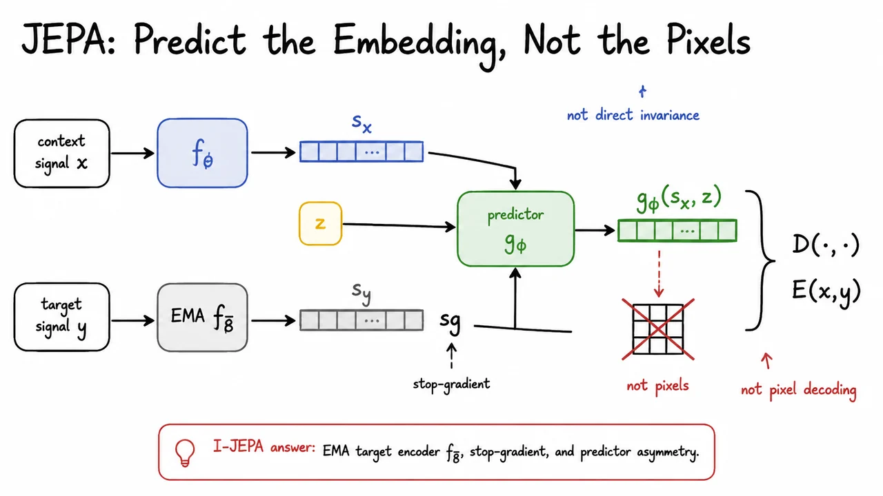
This is the central motivation behind a joint-embedding predictive architecture, or JEPA. Instead of predicting $y$ itself, the model predicts an embedding of $y$. In other words, we still keep the predictive flavor of generative modeling—there is a context $x$, a target $y$, and a notion of compatibility—but we move the target from pixel space into representation space.

From the energy-based viewpoint, the goal is to learn an energy $E(x,y)$ that is low when $x$ and $y$ are compatible and high otherwise. For images, $x$ might be a visible context region and $y$ might be a masked target region. The key design choice is where the comparison happens. A pixel reconstruction method compares a decoded prediction to the raw target pixels. JEPA instead compares a predicted representation to a target representation:

$$s_x=f_\theta(x),\qquad s_y=f_{\bar\theta}(y).$$

Here $f_\theta$ is the context encoder, and $f_{\bar\theta}$ is a target encoder. The context encoder maps the observed part $x$ to a representation $s_x$, while the target encoder maps the target signal $y$ to a representation $s_y$. A predictor $g_\phi$ then uses the context representation, together with conditioning information $z$, to predict the target embedding:

$$E(x,y)=D\big(g_\phi(s_x,z),\operatorname{sg}(s_y)\big).$$

The distance $D(\cdot,\cdot)$ might be a smooth embedding-space loss, and $\operatorname{sg}$ denotes stop-gradient: the target representation is treated as a fixed target for the purpose of this loss. The conditioning variable $z$ is important because the predictor needs to know what it is supposed to predict. In I-JEPA, for example, $z$ can encode information about the location of the masked target block relative to the visible context.

This places JEPA between two familiar families of self-supervised learning methods. Unlike ordinary joint-embedding architectures such as contrastive or invariance-based methods, JEPA does not simply force two views to have the same representation. Direct invariance can be powerful, but it usually depends heavily on hand-designed augmentations: crops, color jitter, blur, and so on. Those augmentations encode assumptions about what should and should not change the semantic content of an image.

JEPA avoids making invariance the whole objective. The model is not told, “these two transformed views must match.” It is instead asked, “given this context and this target position, predict the representation of the missing target.” That difference matters. The prediction problem can preserve spatial and semantic structure that would be erased by overly aggressive invariance constraints.

At the same time, JEPA is also not a standard generative masked model. It does not decode the missing region back into pixels. This avoids rewarding the model for modeling low-level uncertainty that may not help representation learning. If many textures or colors are plausible for a missing patch, a pixel-level objective may penalize the model for failing to guess arbitrary details. A representation-space objective can instead focus on more stable properties: object parts, layout, category-level information, and contextual compatibility.

The subtle danger is collapse. If the target encoder $f_{\bar\theta}$ maps every possible $y$ to the same constant vector, then the prediction task becomes trivial: the predictor can output that constant for every input, yielding low loss without learning useful visual structure. This is the same fundamental risk faced by non-contrastive joint-embedding methods. JEPA must therefore include mechanisms that make the target nontrivial while still avoiding explicit negative pairs or pixel reconstruction.

I-JEPA’s answer is a combination of target-encoder asymmetry, stop-gradient, and EMA updates. The target encoder parameters $\bar\theta$ are not updated directly by backpropagation through the prediction loss. Instead, they are maintained as an exponential moving average of the context encoder parameters. This creates a slowly moving target network:

• the context encoder $f_\theta$ learns through gradient descent;
• the predictor $g_\phi$ learns to map context embeddings to target embeddings;
• the target encoder $f_{\bar\theta}$ evolves more slowly, stabilizing the prediction target;
• stop-gradient prevents the target branch from chasing the predictor in a degenerate way.

So the JEPA objective is predictive, but not generative in pixel space; joint-embedding, but not merely invariant; non-contrastive, but not unconstrained. Its core bet is that predicting latent representations of missing information gives a cleaner semantic learning signal than reconstructing raw observations.

The visual below can be read as a compact summary of this design. The context signal $x$ flows through the online encoder $f_\theta$, producing $s_x$. The target signal $y$ flows through a separate EMA target encoder $f_{\bar\theta}$, producing $s_y$, with a stop-gradient barrier on that branch. The predictor $g_\phi$ receives $s_x$ and conditioning information $z$, then outputs a predicted representation $g_\phi(s_x,z)$.

The important comparison is on the right: the energy $E(x,y)$ is computed by measuring a distance between the predicted embedding and the stopped target embedding. The crossed-out pixel reconstruction cue emphasizes the essential contrast: JEPA is not trying to redraw the missing image patch. It is trying to predict the representation that a stable target encoder assigns to that patch, which is precisely why it can aim for semantic prediction without relying on hand-crafted invariance or low-level pixel decoding.

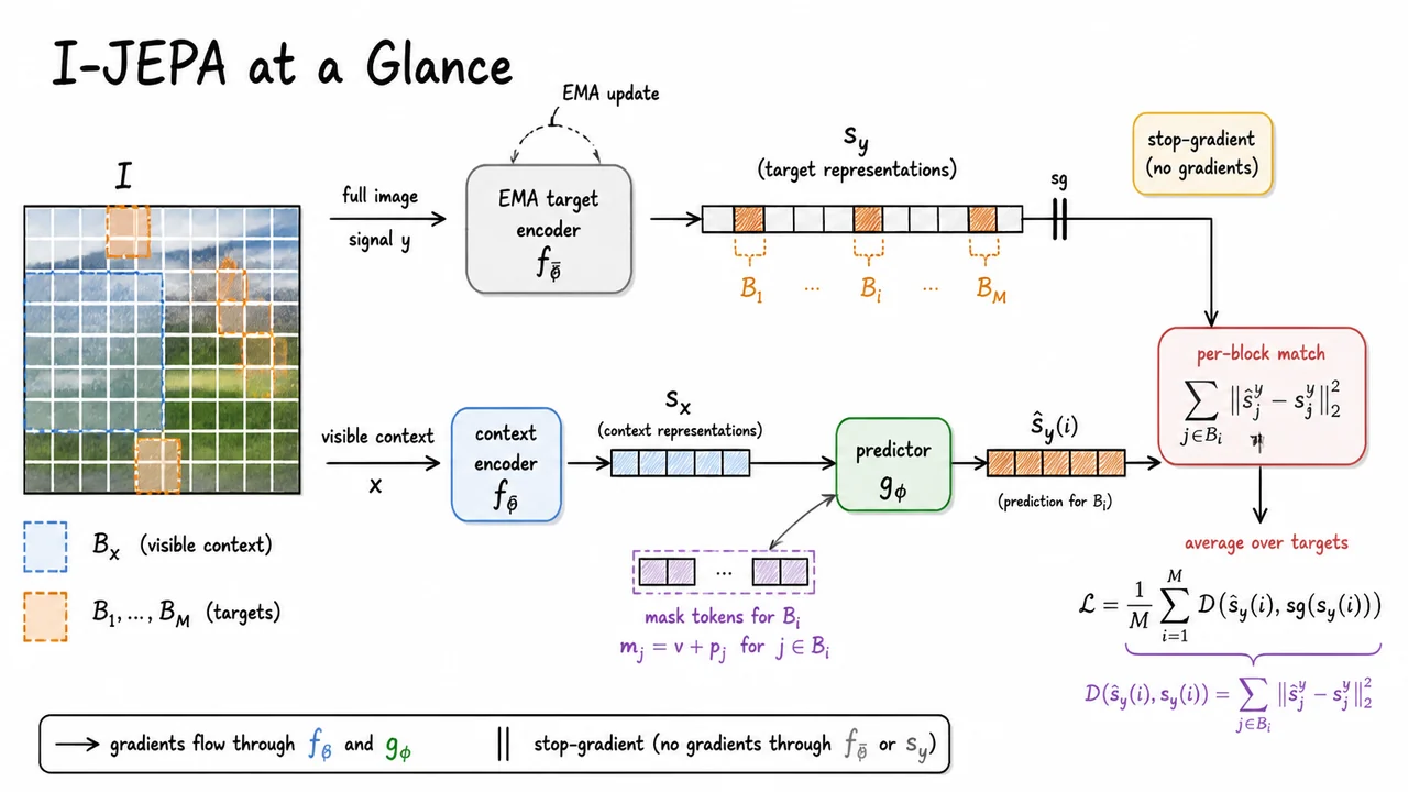
Having separated the JEPA idea from pixel reconstruction, we can now make it concrete for images. I-JEPA keeps the same core principle—predict a missing part of the world in representation space—but instantiates “world,” “context,” and “target” as sequences of image patches. The result looks superficially similar to masked image modeling, because some patches are hidden and later predicted, but the target is not RGB values. The model is asked to predict what an encoder would say about the missing region.

Start with a single image $I$, divided into a patch grid as in a Vision Transformer. I-JEPA samples several target blocks $B_1,\ldots,B_M$, usually spatially contiguous rectangles rather than isolated random patches. It also samples a visible context region $B_x$, with the target blocks removed from what the online encoder sees. This distinction matters: the context encoder must form a representation from incomplete visual evidence, while the target encoder is allowed to process the full image signal and produce representations for the held-out target locations.

The online, or context, branch encodes only the visible context $x$:

$$s_x=f_\theta(x).$$

Here $f_\theta$ is typically a ViT-style encoder applied to the unmasked context patches. The representation $s_x$ should contain enough semantic and geometric information to support predictions about the missing blocks. Crucially, the model is not being rewarded for copying texture or color at the pixel level. It is rewarded for inferring the representation of the missing region from surrounding evidence.

The target branch computes the embeddings that the prediction should match. It uses a separate encoder with parameters $\bar\theta$, maintained as an exponential moving average of the online encoder:

$$s_y=f_{\bar\theta}(y).$$

The target input $y$ corresponds to the image signal from which target-block representations are extracted. In practice, the target encoder provides the representation sequence whose entries at positions in $B_i$ become the prediction targets. Because $\bar\theta$ changes slowly, the target branch acts like a stabilizing teacher rather than a rapidly moving objective. The loss also uses a stop-gradient operation, so optimization does not directly update the target representations to make the task easier.

For each target block $B_i$, I-JEPA gives the predictor two kinds of information: the context representation $s_x$, and a set of positional mask tokens indicating where predictions should be made. A mask token at patch position $j$ is written as

$$m_j=v+p_j,$$

where $v$ is a learned mask-token vector and $p_j$ is the positional embedding for location $j$. This is a subtle but important design choice. The predictor is not merely asked to emit “some missing content”; it is asked to predict the representation that belongs at a specific spatial location. The position token tells the model whether it is predicting, for example, the top-left sky region, the center object region, or the lower background.

The predictor $g_\phi$ then produces target-block representations:

$$\hat{s}_y(i)=g_\phi\left(s_x,\{m_j:j\in B_i\}\right).$$

The predictor can be thought of as a lightweight reasoning module. The context encoder builds the visible-image representation; the mask tokens specify the query locations; the predictor combines both to infer what the target encoder would have represented there. This keeps the difficult part of the task at the semantic-representation level rather than at the pixel-synthesis level.

The pretraining loss compares predicted representations with the stopped target representations:

$$\mathcal{L} = \frac{1}{M}\sum_{i=1}^{M} D\left(\hat{s}_y(i),\operatorname{sg}(s_y(i))\right),$$

with a block-level squared-error distance

$$D\left(\hat{s}_y(i),s_y(i)\right) = \sum_{j\in B_i} \left\| \hat{s}^y_j-s^y_j \right\|_2^2.$$

The operator $\operatorname{sg}(\cdot)$ means stop gradient: the target encoder output is treated as a fixed regression target for the current update. Gradients flow through the predictor $g_\phi$ and the online context encoder $f_\theta$, while the target encoder $f_{\bar\theta}$ is updated only by EMA. This prevents trivial collapse modes where both sides could move together too freely, and it makes the target representation a slowly evolving reference signal.

This setup is designed to avoid two common failure modes in image self-supervision. First, unlike contrastive methods, it does not depend on hand-crafted view augmentations to define invariances. I-JEPA does not need to decide in advance that color jitter, cropping, blur, or other transformations should preserve identity. Second, unlike pixel-reconstruction masked autoencoders, it does not spend most of its capacity modeling low-level details. Predicting encoder representations encourages the model to capture information that is useful for downstream semantic transfer, while still preserving spatial structure through patch-level prediction.

The visual below compactly summarizes this computation as a two-branch pipeline. One branch encodes the full image with the EMA target encoder to produce the representation targets $s_y$. The other branch encodes only the visible context with the online encoder, appends positional mask tokens for each missing block, and sends the combined information to the predictor. The loss is applied only between the predicted block embeddings $\hat{s}_y(i)$ and the corresponding stopped target embeddings $s_y(i)$.

The key thing to notice is the asymmetry: context is incomplete, targets are representational, and the teacher is slow-moving. That asymmetry is what makes I-JEPA a joint-embedding predictive method rather than a generative reconstruction method. It learns by asking: given what is visible, what should the representation of the missing region be?

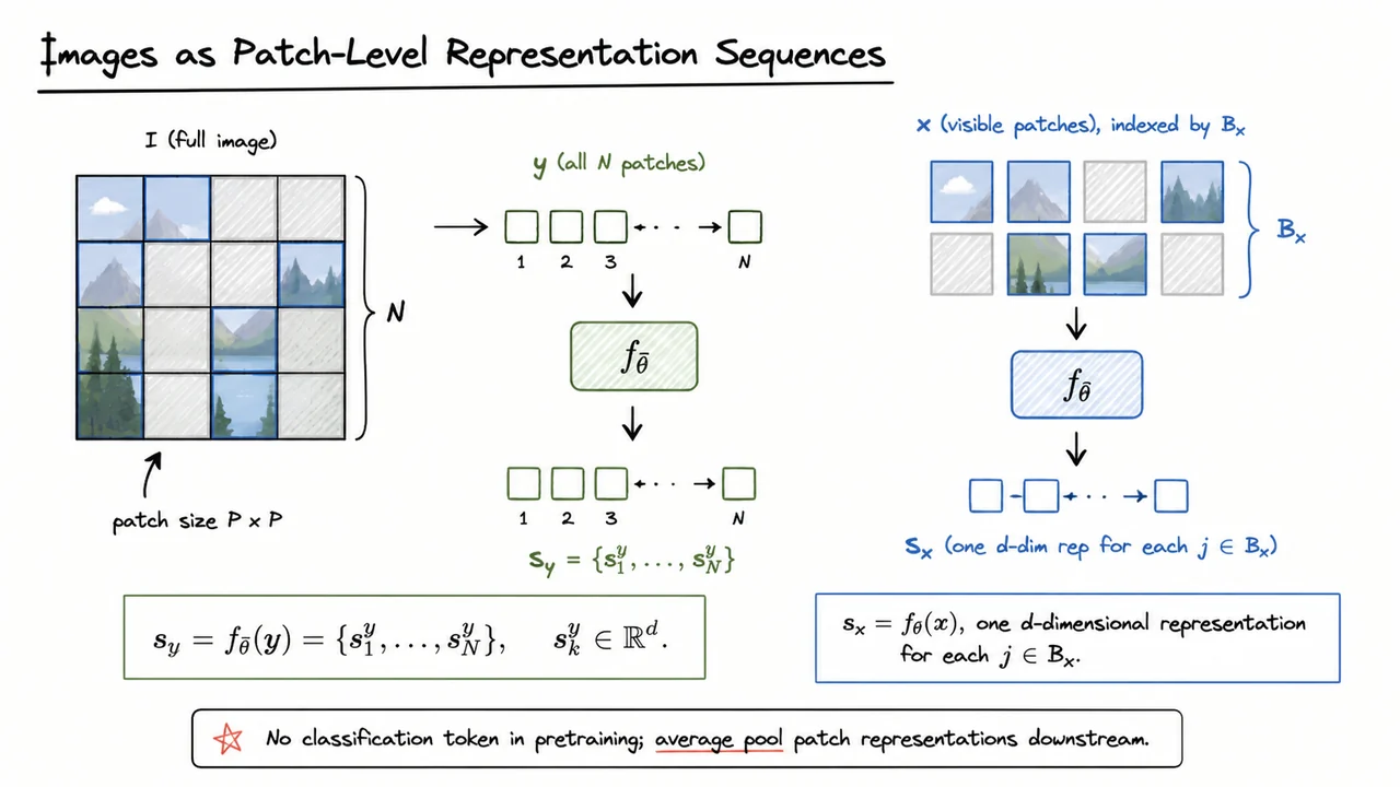
The “at a glance” pipeline is useful, but it hides a crucial modeling choice: I-JEPA does not reason about an image as a continuous pixel canvas once the encoders begin their work. Like a Vision Transformer, it first turns the image into a sequence of patch tokens. That sequence view is what makes masking, indexing, prediction, and pooling mathematically clean.

Suppose an image $I$ is split into $N$ non-overlapping patches, each of spatial size $P \times P$. After patch embedding, the image is no longer treated as one monolithic object; it becomes an ordered collection of local visual units. The order still matters, because each patch has a position, but the model’s internal objects are now patch-level representation vectors rather than raw pixels.

This matters because I-JEPA’s prediction problem is not “fill in missing RGB values.” Instead, it asks: given representations of visible patches, can we predict the representations that another encoder assigns to masked regions? The target branch therefore receives the full image signal $y$ and produces one representation for every patch location:

$$s_y=f_{\bar\theta}(y)=\{s^y_1,\ldots,s^y_N\},\qquad s^y_k\in\mathbb{R}^d.$$

Here $f_{\bar\theta}$ is the target encoder, whose parameters are typically an exponential moving average of the context encoder’s parameters. The output $s_y$ is a length-$N$ sequence, and each element $s^y_k$ is a $d$-dimensional representation associated with patch index $k$. At this point, every patch location has a target representation available, even though only some of those locations will later be selected as prediction targets.

The context branch is different. It receives only the visible part of the image, denoted $x$. More precisely, if $B_x$ is the set of visible context patch indices, then the context encoder processes only those visible patches and returns one representation for each $j\in B_x$:

$$s_x=f_\theta(x),\qquad \text{one } d\text{-dimensional representation for each } j\in B_x.$$

This asymmetry is central. The target encoder sees the full image, while the context encoder sees an incomplete view. But the learning signal is not a pixel reconstruction loss against the original image. The target branch converts the full image into a representation sequence, and the predictor will later try to infer selected target representations from the visible context representations. In other words, masking happens over patch indices, while prediction happens in representation space.

A subtle but important assumption is that patch-level representations contain enough semantic and spatial information to make prediction meaningful. If the representations were too local or too low-level, the task could collapse into texture matching. If they were too invariant too early, the model might lose the spatial detail needed to reason about masked regions. I-JEPA relies on the encoder architecture and the masking scheme to strike a useful balance: the model should learn representations that are predictive of meaningful visual structure without being forced to reproduce every pixel.

This also explains why there is no classification token during I-JEPA pretraining. The objective is defined over patch representations, not over a single global summary token. Later, for downstream tasks that require an image-level feature, one can average pool the learned patch representations. That design keeps the pretraining signal distributed across the image: every patch location can participate as context, target, or both across different masks.

So the key bookkeeping is:

• the full image $y$ produces a target sequence $s_y$ with $N$ patch representations;
• the visible context $x$ produces a shorter sequence $s_x$, indexed only by $B_x$;
• both sequences live in the same $d$-dimensional representation space;
• the pretraining objective will compare predicted target representations to selected elements of $s_y$, not to pixels.

The visual below condenses this indexing story. The full grid of image patches corresponds to the target branch, where all $N$ patch positions are encoded into $s_y=\{s^y_1,\ldots,s^y_N\}$. The highlighted visible patches correspond to the context branch, where only indices in $B_x$ are passed through $f_\theta$ to form $s_x$.

It is worth reading the two branches as complementary views of the same patch sequence. The target branch defines what representations exist at every location; the context branch defines what information the predictor is allowed to use. This separation is what makes the next step possible: constructing target blocks by selecting masked locations from the target-encoder output.

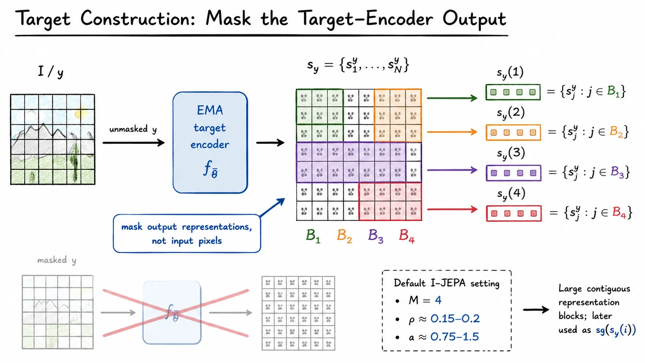
Now that an image has been reframed as a sequence of patch-level representations, the next question is deceptively simple: what exactly should the model predict? In I-JEPA, the answer is not “missing pixels,” and it is not “another randomly augmented view.” Instead, the model predicts parts of a representation sequence produced by a slowly moving target encoder.

This is the first important design move in I-JEPA. The target is constructed by taking the original, uncorrupted image $y$, feeding it through an EMA target encoder $f_{\bar\theta}$, and only then selecting which spatial regions will become prediction targets:

$$s_y=f_{\bar\theta}(y)=\{s^y_1,\ldots,s^y_N\}.$$

Here $N$ is the number of image patches, and $s^y_j$ is the target encoder’s representation for patch position $j$. The notation is intentionally sequence-like: even though the image is two-dimensional, the Vision Transformer has converted it into a structured set of patch embeddings. Each element still corresponds to a spatial location, but it now lives in a learned representation space rather than raw RGB space.

The subtle but crucial point is that the target encoder sees the full image. I-JEPA does not first remove pixels, feed a damaged image into the target network, and ask the context network to imitate that damaged target. Instead, the full image is encoded once, producing a complete representation sequence $s_y$. After that, I-JEPA samples target blocks $B_1,\ldots,B_M$, where each $B_i$ is a set of patch indices, and extracts the corresponding representations:

$$s_y(i)=\{s^y_j: j\in B_i\},\qquad i=1,\ldots,M.$$

So the masking operation happens after the target representation has been computed. The target blocks are subsets of $s_y$, not representations obtained by encoding masked images.

This matters because masking before the target encoder would change the semantic object being predicted. If the target encoder receives an image with holes, then its output at nearby positions may already contain artifacts of the corruption process. The target would no longer be “what the full image says about this region”; it would be “what the encoder says when the image has been partially destroyed.” That is a different learning problem, closer in spirit to denoising or masked reconstruction.

I-JEPA wants something more abstract. The predictor should infer the representation of a missing region from surrounding visible context, but the representation it predicts should be grounded in the unmasked image. This encourages the context encoder and predictor to model higher-level regularities: object parts, scene layout, spatial compatibility, and semantic co-occurrence. In other words, the target should be informative about the image, not about the masking noise.

There is also an anti-collapse motivation here. Joint-embedding methods must avoid trivial solutions where both branches produce constant representations. I-JEPA addresses this partly through architectural asymmetry and EMA target updates, but the target construction also helps: the model is asked to predict multiple large, spatially coherent chunks of a stable representation sequence. Later, these targets are used with a stop-gradient operation, conceptually as

$$\operatorname{sg}(s_y(i)),$$

so the online predictor learns to match the target representations without directly pulling the target encoder toward its own predictions.

The blocks themselves are not tiny isolated patches. In the default I-JEPA setup, the method samples multiple target regions, typically $M=4$, each covering a reasonably large fraction of the image. The scale parameter is roughly $\rho\approx 0.15\text{--}0.2$, and the aspect-ratio range is about $a\approx 0.75\text{--}1.5$. These choices bias the task toward predicting large contiguous semantic regions, rather than solving many small local texture completions.

That design separates I-JEPA from pixel-level masked autoencoding. A masked autoencoder can succeed by learning local statistics useful for reconstructing colors, edges, or textures. I-JEPA deliberately avoids asking for pixels. Its targets are already embedded by a neural network, so the prediction problem lives in representation space. The hope is that this makes the pretraining signal more aligned with downstream semantic transfer: classify, localize, and reason about objects, rather than merely synthesize plausible low-level appearance.

The visual below condenses this construction. Read it left to right: the full image $y$ is first passed through the EMA target encoder $f_{\bar\theta}$, producing the complete representation sequence $s_y$. Only after that do the sampled blocks $B_1,\ldots,B_4$ select subsets of the representation grid, yielding $s_y(1),\ldots,s_y(4)$.

The crossed-out alternative is just as important as the main path. It emphasizes the key rule: do not mask the input to the target encoder. The target branch should encode the unmasked image, and masking should select target representations afterward. This single ordering choice is what lets I-JEPA define prediction targets that are stable, semantic, and detached from pixel reconstruction.

Once the targets have been defined as large semantic blocks, the next question is: what information should the predictor be allowed to condition on? If the context is too small, the task becomes nearly impossible: predicting a large missing region from a few nearby patches may require hallucinating details with little semantic grounding. But if the context includes the target itself, the task becomes trivial leakage. I-JEPA’s context construction is designed to sit precisely between these two failure modes.

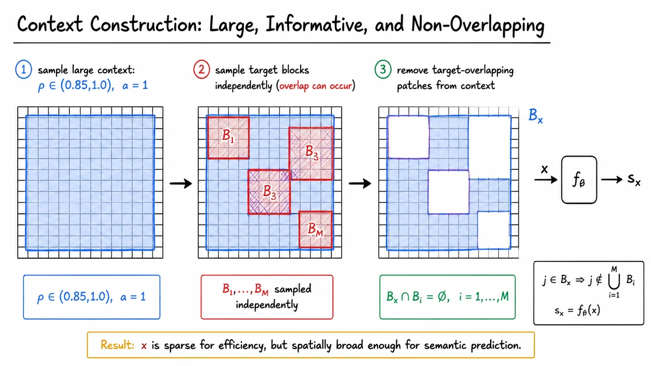
The key design choice is to sample one large context block from the image. Unlike the target blocks, which are multiple and moderately large, the context block is intended to cover most of the image. In the paper’s notation, its scale ratio $\rho$ is sampled close to one, and its aspect ratio is fixed to be square:

$$\rho \in (0.85,1.0), \qquad a=1.$$

Intuitively, this means the context encoder usually sees a broad spatial field: enough of the image to infer object identity, scene layout, pose, and coarse geometry. This is important because I-JEPA is not trying to reconstruct pixels. It is trying to predict representations of missing regions. The best signal for that prediction is not local texture continuity alone, but global semantic consistency.

However, there is a subtle complication. The target blocks $B_1,\ldots,B_M$ are sampled independently, and the initial context block is sampled separately. So, before correction, the context block may overlap with one or more targets. If those overlapping patches were left visible to the context encoder, the predictor could partially “peek” at what it is supposed to predict. That would weaken the learning signal: instead of learning to infer missing-region semantics from surrounding evidence, the model could copy information through shared visible patches.

I-JEPA therefore removes every patch from the context that belongs to any target block. The final visible context set is denoted $B_x$, and it is constrained to be disjoint from each target:

$$B_x \cap B_i = \varnothing, \qquad i=1,\ldots,M.$$

Equivalently, if a patch index $j$ is visible in the context, then it cannot belong to any of the prediction targets:

$$j\in B_x \Rightarrow j\notin \bigcup_{i=1}^{M} B_i.$$

This disjointness condition is easy to overlook, but it is central to the method. I-JEPA wants the prediction problem to be nontrivial: the representation of each target block must be inferred from other image evidence, not read directly. At the same time, the context remains large and informative because it begins as a near-full-image block before the target-overlapping patches are removed.

This also explains why the resulting context can look sparse. The model does not necessarily receive a contiguous crop after masking. Instead, it receives the visible patches from the large context block with holes cut out wherever target blocks lie. The context encoder then processes this sparse visible input:

$$s_x = f_\theta(x).$$

Here, $x$ denotes the visible context patches, and $s_x$ is the context representation produced by the online encoder $f_\theta$. The predictor will later use $s_x$, together with target-position information, to predict the target representations produced by the EMA target encoder.

The design has a useful balance:

• Large context gives enough semantic evidence for meaningful prediction.
• Removed target overlaps prevent shortcut copying.
• Sparse visible patches reduce computation while preserving broad spatial coverage.
• Representation-space prediction keeps the model focused on semantic structure rather than low-level pixel synthesis.

The visual below compactly summarizes this construction as a three-step transformation: first sample a near-full-image context block, then overlay independently sampled target blocks, and finally cut out any target-overlapping patches from the context. The final blue region is not simply “everything except the targets”; it is the original large context block after enforcing the non-overlap constraint.

The arrow from the final context $x$ into the encoder $f_\theta$ emphasizes the role of this construction in the full I-JEPA pipeline. The context encoder only sees the remaining visible patches, producing $s_x$, while the target representations are computed separately from masked target-encoder outputs. This separation is what makes the subsequent prediction step a genuine joint-embedding prediction problem rather than a disguised reconstruction or copying task.

Having constructed a context region that is large, informative, and non-overlapping with the targets, I-JEPA now faces a precise question: what exactly should the predictor be asked to produce? The context encoder has seen only the visible context block $B_x$, so its output $s_x$ contains information about the observed part of the image. But the model still needs to know which missing locations it is supposed to reason about. Without that information, “predict the target” is under-specified: the same context could surround many possible missing regions.

This is where I-JEPA’s predictor departs from a pixel-reconstruction mindset. It does not ask the model to synthesize RGB patches, textures, or low-level details. Instead, it asks the predictor to produce representation vectors corresponding to specified missing patch locations. The missing locations are not represented by pixels; they are represented by target-position tokens that tell the predictor, “predict the representation that should live here.”

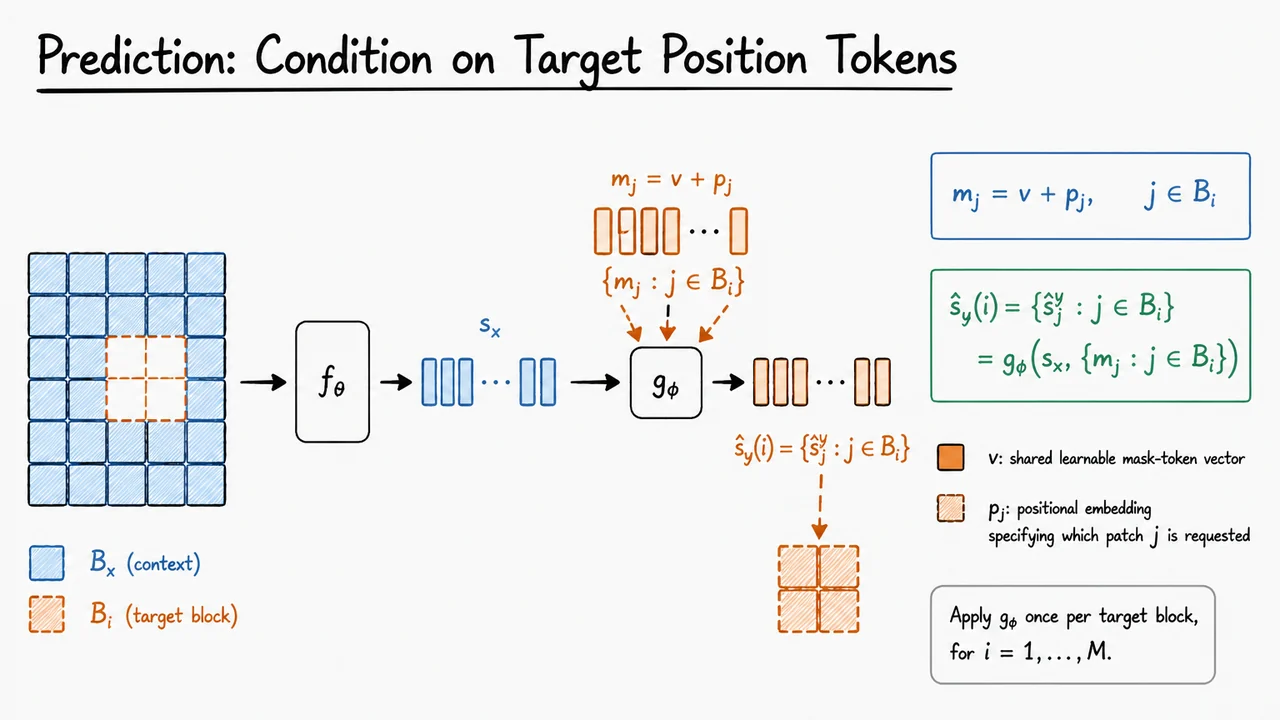
For each target block $B_i$, I-JEPA creates one token per target patch. If $j$ indexes a patch inside the target block, the corresponding predictor input token is

$$m_j = v + p_j, \qquad j \in B_i .$$

Here, $v$ is a shared learnable mask-token vector, while $p_j$ is a positional embedding identifying the requested patch location. The shared vector $v$ says, in effect, “this is a missing target token,” while $p_j$ says which missing token it is. This is a subtle but important distinction: the predictor is not given the target content, only the target coordinates.

The predictor $g_\phi$ then receives two sources of information:

• the context representation $s_x$, produced from the visible context $B_x$;
• the set of target-position tokens $\{m_j : j \in B_i\}$, one for each patch in the target block.

Its job is to output one predicted representation per requested target patch:

$$\hat{s}_y(i) = \{\hat{s}^y_j : j \in B_i\} = g_\phi\!\left(s_x,\{m_j : j \in B_i\}\right).$$

So the predictor is not merely “filling in a mask.” It is performing a conditional representation prediction: given what is visible, and given a query specifying a set of missing positions, infer the latent representations that the target encoder would have produced at those locations.

This design solves an important ambiguity. Suppose the context contains the left side of an object, a bit of background, and some global scene cues. The representation appropriate for a missing patch above the object may differ greatly from the representation appropriate for a missing patch inside the object or below it. If the predictor only received $s_x$, it would have no explicit way to distinguish these requests. The positional token $p_j$ turns the prediction into a query: predict the target representation at location $j$, conditioned on the context.

It also matters that $g_\phi$ is applied once per target block, not once for the whole image. For target blocks $B_1,\ldots,B_M$, the same predictor processes each block’s position tokens together with the same context representation. This encourages the predictor to reason about each missing region as a structured block, rather than as isolated independent pixels. The block-level formulation preserves some spatial coherence while still avoiding pixel-level reconstruction.

There is a useful way to interpret the roles of the components:

• $f_\theta$, the context encoder, builds a representation of what is visible.
• $m_j = v+p_j$ specifies a missing-location query.
• $g_\phi$ combines the context and the query tokens.
• $\hat{s}^y_j$ is the predicted representation for the target patch $j$.

The failure mode this avoids is asking the network to spend capacity on irrelevant visual detail. If the target were pixels, the model might learn to predict local texture statistics, color continuity, or other low-level cues. If the target-position tokens were absent, the model would not know which representation it was being asked to infer. I-JEPA’s predictor sits between these extremes: it is spatially specific, but its target is semantic representation space rather than raw image space.

The visual below compactly summarizes this computation. The context patches are encoded into $s_x$; the missing target block contributes no content, only learned position-conditioned mask tokens $m_j=v+p_j$. These two streams meet inside the predictor $g_\phi$, which outputs a row of predicted target representations $\hat{s}_y(i)$ aligned with the requested target patches.

This is the final step before defining the training signal. At this point, I-JEPA has produced predictions in representation space, but we have not yet said what they are compared against or how the target representations remain stable during learning. That is the role of the loss and the EMA target encoder.

Once the predictor has been given both the context representation and the target position tokens, the remaining question is deceptively simple: what exactly should its output be trained to match? I-JEPA’s answer is the central design choice of the method. The prediction is not compared to raw pixels, and it is not trained to reconstruct missing patches in image space. Instead, the predictor is asked to match the latent representation that a separate target encoder assigns to the masked target block.

This is where I-JEPA differs sharply from generative masked image modeling. In a pixel-reconstruction method, the model must explain low-level details: texture, color, edges, local statistics, and sometimes even compression artifacts. Those targets are easy to define but not necessarily aligned with semantic understanding. I-JEPA deliberately avoids this by making the target live in representation space. The hope is that predicting what the missing region means is more useful than predicting exactly what the missing pixels look like.

For a given target block $B_i$, the target encoder produces representations

$$s_y(i)=\{s^y_j : j\in B_i\},$$

while the predictor produces corresponding predictions

$$\hat{s}_y(i)=\{\hat{s}^y_j : j\in B_i\}.$$

The discrepancy for one target block is simply a squared Euclidean distance over the patch-level embeddings in that block:

$$D(\hat{s}_y(i),s_y(i)) = \sum_{j\in B_i} \|\hat{s}^y_j-s^y_j\|_2^2.$$

This loss is intentionally plain. There is no decoder, no pixel likelihood, no contrastive negative sampling, and no hand-designed view transformation to define invariance. The architecture itself creates the prediction task: infer the target-block representation from the visible context and the target location.

Across $M$ sampled target blocks, I-JEPA averages these blockwise discrepancies:

$$\mathcal{L} = \frac{1}{M} \sum_{i=1}^{M} D\bigl(\hat{s}_y(i),\operatorname{sg}(s_y(i))\bigr).$$

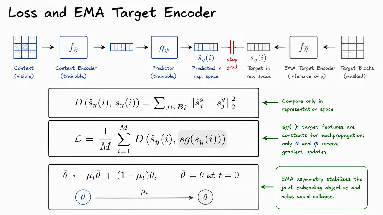
The $\operatorname{sg}(\cdot)$ operator is crucial. It denotes stop-gradient: during backpropagation, the target features are treated as constants. Gradients flow into the context encoder parameters $\theta$ and predictor parameters $\phi$, but not directly into the target encoder output used as the regression target. Without this asymmetry, both sides of the prediction problem could move together in unhelpful ways.

That point is worth lingering on, because it is one of the main stability mechanisms in joint-embedding methods. If both the predictor and the target encoder were updated by the same loss at the same time, the system could reduce the loss through degenerate coordination rather than meaningful representation learning. In the extreme, both networks could drift toward constant or collapsed embeddings, making prediction trivial but useless. The stop-gradient prevents the target branch from chasing the online branch through the loss.

However, I-JEPA does not keep the target encoder fixed forever. A permanently frozen target encoder would provide a stable objective, but it would not improve as the online representation improves. Instead, the target encoder is updated as an exponential moving average of the online context encoder:

$$\bar\theta \leftarrow \mu_t\bar\theta + (1-\mu_t)\theta, \qquad \bar\theta=\theta\text{ at }t=0.$$

Here $\theta$ denotes the trainable context encoder parameters, while $\bar\theta$ denotes the target encoder parameters. The momentum coefficient $\mu_t$ is usually close to $1$, so the target encoder evolves slowly. This creates a teacher-like branch that is not directly optimized by the current minibatch loss, but still tracks the long-term trajectory of the learned representation.

The result is a carefully balanced form of asymmetry:

• the online path $(f_\theta, g_\phi)$ receives gradients and learns to predict;
• the target path $f_{\bar\theta}$ produces the representation target but is stop-gradiented;
• the EMA update lets the target path improve slowly without becoming an unstable moving target.

This combination is one reason I-JEPA can use a simple representation-space regression loss without explicit negatives. The target branch is neither an adversary nor a decoder; it is a slowly updated reference representation. The predictor must learn to map from partial context to the latent representation of missing regions, while the EMA mechanism keeps that target coherent across training.

The visual below compactly organizes this mechanism: a trainable blue path produces $\hat{s}_y(i)$, a slowly updated gray target path produces $s_y(i)$, and a stop-gradient barrier prevents the loss from directly updating the target features. The equations in the center summarize the two levels of averaging: first over the patches $j\in B_i$ inside one target block, then over the $M$ target blocks sampled from the image.

The bottom EMA update is the final piece of the loop. It makes clear that the target encoder is not learned by ordinary gradient descent on the loss; instead, it is pulled toward the context encoder over time. That small implementation detail is conceptually large: it is what turns representation-space prediction into a stable self-supervised objective rather than a symmetric regression problem prone to collapse.

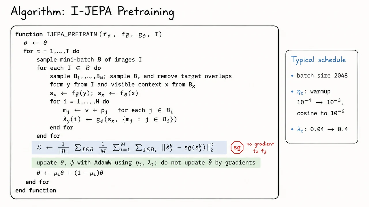
With the loss and EMA target encoder in place, the full I-JEPA training algorithm becomes surprisingly compact. The key point is that nothing in the loop asks the model to reconstruct pixels. Instead, each iteration asks: given a visible context from an image, can the predictor infer the target encoder’s representations at several masked spatial regions? This is why I-JEPA sits between contrastive joint-embedding methods and generative masked autoencoders: it predicts missing information, but it predicts it in representation space, not RGB space.

For each image $I$, I-JEPA samples two kinds of masks. First, it samples $M$ target blocks $B_1,\ldots,B_M$, usually fairly large contiguous regions. These are the regions whose latent representations the model will try to predict. Second, it samples a context mask $B_x$, which determines which patches remain visible to the context encoder. Importantly, target regions are removed from the context, so the context encoder cannot simply “peek” at the answer. The model must use surrounding visible evidence and learned semantic regularities to infer what the target representations should be.

The image is therefore split conceptually into a target view $y$ and a context view $x$. The target view is passed through the EMA target encoder $f_{\bar\theta}$, while the context view is passed through the trainable context encoder $f_\theta$:

$$s_y = f_{\bar\theta}(y), \qquad s_x = f_\theta(x).$$

The target representation $s_y$ provides the regression target, but it is treated as a fixed quantity for the gradient update. This is the role of the stop-gradient operator. During backpropagation, the loss updates only the context encoder $f_\theta$ and predictor $g_\phi$, not the target encoder $f_{\bar\theta}$.

For each target block $B_i$, the predictor receives the context representation $s_x$ along with a set of mask tokens indicating where the missing target patch representations should be predicted. A mask token at spatial location $j$ is formed as

$$m_j = v + p_j,$$

where $v$ is a learned mask embedding and $p_j$ is the positional embedding for location $j$. This detail is small but important: the predictor is not merely asked to produce “some missing feature”; it is asked to produce the feature corresponding to a particular spatial location. Without positional information, block prediction would be ambiguous, especially when multiple target regions are sampled from the same image.

The predictor then outputs estimates $\hat{s}^y_j$ for the target representations at the masked locations. The training objective averages the squared error across images, target blocks, and locations inside each block:

$$\mathcal{L} = \frac{1}{|\mathcal{B}|} \sum_{I\in\mathcal{B}} \frac{1}{M} \sum_{i=1}^{M} \sum_{j\in B_i} \left\| \hat{s}^y_j - \operatorname{sg}(s^y_j) \right\|_2^2.$$

This objective looks like a plain regression loss, but its behavior depends heavily on the architecture around it. If the target encoder were updated directly by gradients from this loss, the system could drift toward degenerate solutions more easily. Instead, I-JEPA uses the familiar teacher-student stabilization mechanism: after each gradient update to $\theta$ and $\phi$, the target encoder parameters are moved slowly toward the context encoder parameters:

$$\bar\theta \leftarrow \mu_t \bar\theta + (1-\mu_t)\theta.$$

This EMA update makes $f_{\bar\theta}$ a slowly evolving teacher. The target network is not frozen forever, but it changes smoothly enough that the prediction task remains stable. In practice, this matters because the predictor is chasing representations that are themselves learned. If the target moved too quickly, the loss would become noisy and self-referential; if it never moved, the model would be limited by an outdated teacher. EMA is the compromise.

The full pretraining loop is therefore a repeated sequence of four operations:

• sample masks: choose multiple target blocks and a non-overlapping visible context;
• encode views: compute target features with $f_{\bar\theta}$ and context features with $f_\theta$;
• predict target representations: use $g_\phi$ and positional mask tokens to predict missing block embeddings;
• update parameters: optimize $\theta,\phi$ by AdamW, then update $\bar\theta$ only by EMA.

There are a few subtle failure modes hidden in this otherwise simple loop. If the target blocks are too small or too local, the prediction task can become low-level and texture-driven. If the context includes too much of the target region, the task becomes trivial. If the target encoder is not stop-gradient/EMA stabilized, the model may learn shortcuts or unstable representations. I-JEPA’s masking strategy, representation-space target, and EMA teacher are therefore not independent tricks; they work together to make prediction semantic rather than pixel-copying.

The visual below condenses this procedure into a pseudocode-style training loop. The highlighted loss line is the heart of the method: predictions from the context branch are matched to stop-gradient target representations, not pixels. The highlighted EMA line marks the second half of the update rule: after AdamW changes the context encoder and predictor, the target encoder follows through the moving-average update rather than ordinary backpropagation.

The side callout with batch size, learning-rate schedule, and weight-decay schedule is also worth noticing. I-JEPA’s algorithmic idea is simple, but its empirical strength depends on scaling it cleanly: large batches, scheduled optimization, multi-block masking, and a slowly updated target encoder make the representation-prediction objective work reliably at ImageNet scale and beyond.

After spelling out the training loop, it is worth pausing on a practical question: why is this loop affordable at ImageNet scale, especially for large ViTs? I-JEPA is not merely “MAE but predicting embeddings.” Its efficiency comes from a set of architectural choices that keep the expensive computation concentrated where it matters: the context encoder processes only visible patches, the target encoder is stabilized by EMA and kept out of backpropagation, and the predictor is intentionally narrow.

The central asymmetry is between context computation and target computation. The online encoder $f_\theta$ receives only the visible context block $B_x$, not the full image. If an image is split into $N$ patches, and only a subset is retained as context, then the self-attention cost of the online ViT scales with the number of context tokens rather than all $N$ tokens. Since ViT attention is quadratic in token count, this matters a great deal: reducing tokens is not just a linear savings in input size, but a larger reduction in attention interactions.

The target side has a different role. The EMA encoder $f_{\bar\theta}$ computes target representations

$$s_y=\{s^y_1,\ldots,s^y_N\},$$

or at least the representations from which the target block embeddings are selected. These target features serve as the prediction targets, but gradients do not flow through $f_{\bar\theta}$. This is crucial: the target encoder provides a slowly moving representation space, rather than a simultaneously learned target that can collapse or chase the predictor too aggressively. The EMA update makes $f_{\bar\theta}$ a temporally smoothed version of $f_\theta$, giving the predictor a stable semantic coordinate system to aim for.

This design has a subtle but important assumption: the representation space produced by the target encoder is already meaningful enough, or becomes meaningful quickly enough, that predicting missing-region embeddings encourages semantic abstraction. If the target representation were noisy, unstable, or overly local, then predicting it would not necessarily teach the context encoder useful invariances. The EMA mechanism reduces this instability, and the use of large target blocks pushes the task away from trivial patch-level texture matching.

The predictor $g_\phi$ is where I-JEPA pays its extra cost. For each target block $B_i$, it receives the context representation $s_x$ and mask/location information $\{m_j\}_{j\in B_i}$, then predicts the representation of that target region:

$$\hat{s}_y(i)=g_\phi(s_x,\{m_j\}_{j\in B_i}).$$

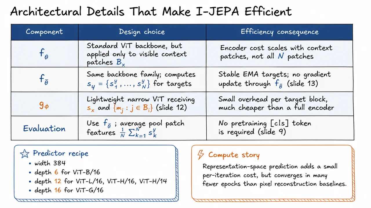
But $g_\phi$ is not a second full-scale image encoder. It is a lightweight narrow ViT, deliberately smaller than the backbone. In the paper’s configurations, the predictor width is $384$, with depth increasing as the backbone scales: depth $6$ for ViT-B/16, depth $12$ for ViT-L/16, ViT-H/16, and ViT-H/14, and depth $16$ for ViT-G/16. This makes the predictor expressive enough to reason over context and locations, but not so powerful that it dominates the training cost.

There is also a useful modeling constraint hidden in this choice. Because the predictor is narrow, it cannot simply behave like a full reconstruction engine. It must rely on the semantic information encoded in $s_x$, plus the positional hints supplied by the mask tokens. That encourages the online encoder to produce context features that are predictive of what is missing at a high level. A too-large predictor could potentially absorb much of the burden itself, weakening the pressure on $f_\theta$ to learn general-purpose representations.

At evaluation time, I-JEPA also avoids depending on a special pretraining classification token. Instead, the EMA encoder $f_{\bar\theta}$ is used as the representation extractor, and patch features are average pooled:

$$\frac{1}{N}\sum_{k=1}^{N}s^y_k.$$

This is a clean consequence of the training objective: the model has learned to organize information across patch-level embeddings, so a pooled representation is already meaningful for downstream transfer. It also avoids coupling the method to a particular pretraining $[cls]$ token behavior, which can be brittle across architectures or evaluation protocols.

The efficiency story is therefore not that I-JEPA has zero overhead. Representation-space prediction does add extra computation through $g_\phi$, and the EMA target encoder must still be evaluated. The point is that this overhead is strategically placed. Compared with pixel reconstruction methods, I-JEPA avoids decoding high-dimensional RGB targets and avoids spending many epochs learning low-level image statistics. The paper’s empirical claim is that this tradeoff pays off: a modest per-iteration cost can be offset by substantially faster convergence in terms of training epochs.

A compact way to remember the design is:

• Online encoder $f_\theta$: expensive backbone, but only on visible context patches.
• Target encoder $f_{\bar\theta}$: stable EMA backbone, no gradient path.
• Predictor $g_\phi$: narrow ViT, predicts missing-region embeddings rather than pixels.
• Evaluation: average pooled EMA patch features, no required pretrained $[cls]$ token.

The visual below condenses these implementation choices into a table: each row isolates one component, the design decision behind it, and the resulting efficiency consequence. The key pattern is that I-JEPA spends full ViT capacity on representation learning, not on pixel decoding, and uses the predictor as a small bridge between visible context and missing target embeddings.

The two callouts at the bottom are especially useful for keeping scale in mind. The predictor recipe gives the concrete width/depth choices used in the paper, while the compute story summarizes the broader tradeoff: I-JEPA accepts a small representation-space prediction overhead, but gains efficiency by avoiding full-image online encoding and long pixel-reconstruction pretraining schedules.

After the architectural details, it is useful to make the mechanics concrete. I-JEPA can sound abstract because it predicts representations rather than pixels, and because the masking happens over spatial blocks rather than isolated random tokens. But for a standard ViT input, the bookkeeping is quite simple: we take one image, divide it into patches, choose several target regions, remove those regions from the context, and train a predictor to infer the target encoder’s latent vectors at the missing positions.

Consider a single image $I\in\mathbb{R}^{224\times224\times3}$ processed by a ViT-H/14 backbone. With patch size $P=14$, the image becomes a $16\times16$ grid of patch tokens:

$$16\times16 \text{ patches} \quad\Rightarrow\quad N=256.$$

So the “world” for this example is a sequence of 256 spatial tokens. Each token corresponds to a $14\times14$ patch, but I-JEPA’s loss is not asking the model to reconstruct those $14\times14$ RGB values. Instead, the target encoder maps the full image into a grid of latent semantic features $s^y_j$, and the context encoder maps a masked image context into latent features $s_x$. The prediction task lives entirely in this representation space.

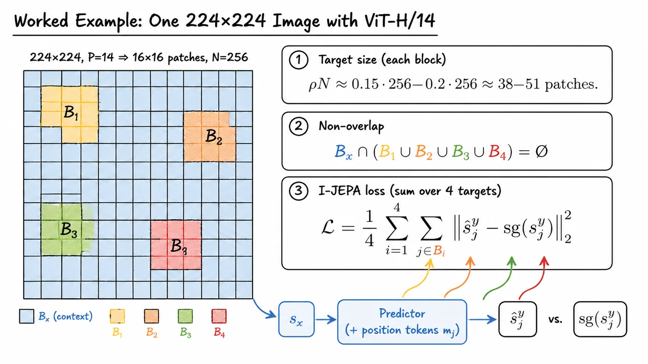
Now suppose we sample $M=4$ target blocks, $B_1,\dots,B_4$. These are not tiny single-patch masks; they are relatively large contiguous regions. In the I-JEPA setup, each target block often covers a scale around $\rho\approx0.15\text{--}0.2$ of the image tokens, so for $N=256$,

$$\rho N \approx 0.15\cdot256\text{--}0.2\cdot256 \approx 38\text{--}51 \text{ patches.}$$

That size matters. If the targets were too small, the task could collapse into local texture interpolation: infer a missing patch from its immediate neighbors. By making each target region large, I-JEPA encourages the predictor to use broader semantic context: object shape, scene layout, part-whole relationships, and other regularities that are more useful for transfer than pixel-level detail.

The context block $B_x$ is sampled to be large as well, but with one crucial constraint: it must exclude all target locations. Formally,

$$B_x \cap (B_1\cup B_2\cup B_3\cup B_4)=\varnothing.$$

This non-overlap condition is easy to overlook, but it is central to the method. If target tokens leaked into the context encoder, the predictor could partially copy or shortcut the target representation. I-JEPA’s objective only makes sense if the prediction must be made from available surrounding context plus the positional information indicating where the missing target features should be predicted.

For each target block $B_i$, the predictor receives two kinds of information. First, it receives the context representation $s_x$, computed from the visible context patches. Second, it receives target position tokens $m_j$, which tell the predictor which spatial locations it should produce predictions for. The predictor then outputs $\hat{s}^y_j$, an estimate of the target encoder’s representation at each masked target position $j\in B_i$.

The loss averages the squared representation-space error over the four target blocks:

$$\mathcal{L} = \frac{1}{4} \sum_{i=1}^{4} \sum_{j\in B_i} \left\| \hat{s}^y_j-\operatorname{sg}(s^y_j) \right\|_2^2.$$

The $\operatorname{sg}(\cdot)$ operator indicates stop-gradient: the target representation $s^y_j$ is treated as a fixed regression target for this update. In practice, the target encoder is updated by an exponential moving average of the context encoder, not by direct backpropagation through this loss. This is part of what stabilizes the joint-embedding setup and prevents the target branch from simply chasing the predictor.

A useful way to read the objective is: “From the non-overlapping visible region $B_x$, predict what the target encoder would have represented inside each large hidden region $B_i$.” The model is not rewarded for drawing the missing pixels. It is rewarded for matching the latent features produced by a slowly moving teacher network. That distinction is exactly why I-JEPA sits between contrastive joint-embedding methods and generative masked modeling: it has a predictive masked objective, but the target is semantic representation rather than raw observation.

The visual below condenses this example into the two pieces of bookkeeping that matter most. On the left is the $16\times16$ patch grid induced by a $224\times224$ image with $P=14$. Four warm-colored target blocks occupy large contiguous regions, while the pale blue context region covers much of the remaining grid but deliberately leaves holes where the targets were removed.

On the right, the same computation is summarized algebraically: target blocks contain roughly $38\text{--}51$ patches each, the context and targets are disjoint, and the final objective averages squared errors over all target positions across the four blocks. The arrows from context to prediction and from target blocks to the loss emphasize the central I-JEPA idea: predict missing representations at specified spatial locations using only the visible context.

After walking through a single 224×224 image with ViT-H/14, it is useful to step back and ask what kind of self-supervised learning algorithm I-JEPA actually is. The mechanics look partly familiar: we mask regions, encode visible context, and predict something about the hidden parts. But the target is not pixels, and the method does not rely on producing two heavily augmented views of the same image. That places I-JEPA in an interesting middle ground between joint-embedding methods and masked predictive methods.

A helpful way to compare SSL methods is through the “energy” perspective introduced earlier. Most methods define some compatibility score, distance, or loss between a prediction and a target. The crucial design choices are:

• What is the target? Pixels, discrete tokens, another view’s representation, or latent features of hidden content?
• Where is prediction performed? Image space, token space, or representation space?
• How is collapse avoided? Negatives, reconstruction constraints, teacher-student asymmetry, stop-gradients, EMA targets, or architectural bottlenecks?

I-JEPA’s objective can be written as a prediction in representation space. For a target block $B_i$, the target encoder produces patch-level representations $s^y_j$, and the representation target for that hidden block is

$$s_y(i)=\{s^y_j:j\in B_i\}.$$

The predictor receives the encoded visible context together with mask/block information and outputs $\hat{s}_y(i)$, a prediction of the missing block’s latent representation. The training loss compares the predicted latent block with the stop-gradient target:

$$D(\hat{s}_y(i),\operatorname{sg}(s_y(i))).$$

This equation captures the central distinction: I-JEPA is not asked to reconstruct RGB values. It is asked to infer the semantic representation that a target encoder would assign to the hidden region.

That difference matters because pixel reconstruction and representation prediction impose different pressures on the model. In MAE-style masked autoencoding, the model must recover low-level visual details: color, texture, local edges, and other information needed to synthesize missing patches. This is a powerful pretraining signal, but it can spend capacity on details that are not always useful for downstream semantic recognition. In contrast, I-JEPA’s target lives in the embedding space of a learned encoder, so the prediction problem can ignore some nuisance variation and emphasize higher-level structure.

At the same time, I-JEPA is not simply another augmented-view invariance method like SimCLR or DINO. Those methods create two or more transformed views of the same image and encourage their representations to agree. This has been extremely effective, but it depends heavily on hand-crafted augmentations. The augmentations encode assumptions about what should be invariant: color jitter should not matter, crops should preserve identity, blur should not change class, and so on. These assumptions often work well for natural-image classification, but they are still human-designed priors.

I-JEPA tries to avoid both of these dependencies. It avoids pixel-level reconstruction targets, and it avoids strong hand-crafted view augmentations. Instead, it uses one image $I$, masks out target blocks, and asks whether the visible context contains enough information to predict the latent representation of the hidden content. In that sense, it is predictive like masked modeling but non-generative like joint embedding.

The collapse problem also looks different depending on the family of methods. If a representation learner simply minimizes distance between two embeddings, a constant representation can become a trivial solution unless something prevents it. SimCLR avoids this with contrastive negatives. DINO uses a teacher-student setup with centering and sharpening. MAE avoids collapse because a constant output cannot reconstruct diverse missing pixels. BEiT uses a fixed tokenizer to provide nontrivial discrete targets. I-JEPA uses a combination of EMA target encoder, stop-gradient, and predictor asymmetry: the target network changes slowly, gradients do not directly update the target representations, and the predictor must map context embeddings to hidden-block embeddings.

This is why I-JEPA is best understood as a hybrid at the level of principle, not as a mixture of losses. It borrows the representational target style of joint-embedding learning, but it borrows the spatial prediction setup of masked modeling. The key object is not an augmented pair $(x_1,x_2)$, nor a pixel patch $x_{B_i}$, but a hidden-block representation $s_y(i)$. The model learns by making the context representation predictive of these latent target blocks.

The visual comparison below condenses this taxonomy. The important axes are the target type, whether strong view augmentations are required, the prediction space, and the main anti-collapse mechanism. Reading across the I-JEPA row should make the contrast clear: one image, hidden target blocks, representation-space prediction, and EMA/stop-gradient stabilization.

It is especially useful to compare I-JEPA with nearby methods rather than only with distant ones. Compared with MAE and BEiT, it changes the target from pixels or tokens to learned representations. Compared with SimCLR and DINO, it removes the need for paired augmented views. Compared with data2vec, it shares the idea of teacher representations as targets, but I-JEPA emphasizes structured multi-block prediction from image context within a joint-embedding predictive architecture.

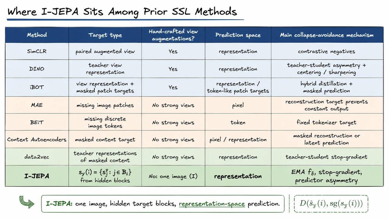
Having placed I-JEPA among contrastive, generative, and hybrid self-supervised methods, the next question is more mundane but absolutely crucial: what representation is actually being evaluated? In self-supervised learning, a few percentage points can hinge not only on the pretraining objective, but also on whether we freeze the backbone, fine-tune it, average spatial tokens, concatenate layers, or accidentally evaluate an auxiliary module that was never meant to be the final representation.

For I-JEPA, the representation used downstream comes from the EMA target encoder, not from the predictor. Recall that pretraining contains an online context encoder, a predictor, and a slowly updated target encoder. The predictor is trained to map context representations toward target-block representations, but it is an auxiliary training-time module. At evaluation time, the paper treats the target encoder as the learned visual representation:

$$s_y=f_{\bar\theta}(y)=\{s^y_1,\ldots,s^y_N\}.$$

Here $y$ is an input image, $f_{\bar\theta}$ is the EMA target encoder, and the output is a sequence of patch-level embeddings. The bar over $\theta$ matters: $\bar\theta$ denotes the exponential-moving-average parameters, which tend to be smoother and more stable than the instantaneous online parameters. This is analogous to the role of a teacher network in many self-supervised systems: the model used for evaluation is the slowly accumulated representation, not the transient training head.

For image-level classification protocols, I-JEPA converts the patch sequence into a single vector by average pooling the patch outputs. In other words, if the encoder emits $N$ patch embeddings, the downstream classifier usually receives something like

$$\bar{s}_y=\frac{1}{N}\sum_{i=1}^{N}s_i^y.$$

This choice is simple, but it encodes an assumption: semantic information should be distributed across the patch tokens in a way that survives global pooling. That is a reasonable assumption for ImageNet-style object recognition, where the label often corresponds to a dominant object or scene-level concept. It is less obvious for tasks requiring fine spatial relationships, which is why the paper also reports local and low-level transfer evaluations.

The protocols in the paper are designed to answer different questions. A linear probe freezes the pretrained encoder and trains only a linear classifier on top. This is a deliberately restrictive test: if a frozen representation supports high linear accuracy, then the semantic structure was already present before supervised adaptation. By contrast, a low-shot protocol asks how efficiently a method adapts when labels are scarce. These are related but not identical notions. A representation can be linearly separable under full labels yet still adapt poorly with few labels, or it can require some fine-tuning but become label-efficient once adapted.

This distinction is especially important when comparing I-JEPA to methods with different evaluation recipes. The paper reports several protocol families:

• ImageNet linear evaluation: freeze the encoder and train a classifier using the full ImageNet-1k training set.
• ImageNet 1% evaluation: use only about 1% of ImageNet labels, with the exact freezing or fine-tuning recipe depending on the method being compared.
• Transfer linear probes: freeze the encoder and train linear classifiers on other labeled datasets.
• CLEVR Count/Distance evaluations: test whether the learned features preserve more local or low-level information useful for structured visual reasoning tasks.

The failure mode to watch for is treating all of these numbers as if they measure the same property. They do not. ImageNet linear accuracy mostly measures global semantic separability. Low-shot ImageNet performance measures label efficiency under a particular adaptation recipe. Transfer probes measure whether semantic structure generalizes beyond the source distribution. CLEVR-style tasks probe whether the representation retains information about counting, geometry, and object relations, which may be weakened by representations optimized only for global category discrimination.

There is also a small but meaningful implementation detail: some evaluation recipes concatenate outputs from the last four encoder layers before pooling. This can help because different layers encode different levels of abstraction. Later layers may be more semantic but less spatially precise; slightly earlier layers may preserve more local structure. Concatenating them gives the linear probe access to a richer mixture of features without changing the pretrained encoder itself.

The visual below condenses these distinctions into a protocol map. Its main purpose is to keep the evaluation axes separate: which network is frozen, how many labels are used, and what property the resulting number should be interpreted as measuring. The central equation reminds us that the evaluated object is $f_{\bar\theta}$, the EMA target encoder, producing patch-level outputs that are pooled for downstream use.

Read the table as a guardrail for the empirical section that follows. When the next results report ImageNet linear and 1% low-shot performance, the numbers should not be read merely as “accuracy.” They are evidence about different aspects of the representation: frozen semantic quality in one case, and label-efficient adaptation in the other.

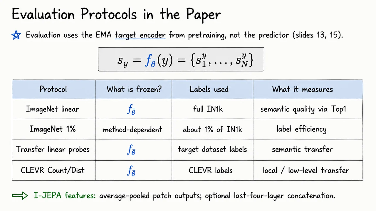
With the evaluation protocol fixed, the ImageNet numbers become more than a leaderboard entry: they are a test of what kind of information I-JEPA has learned during pretraining. Linear probing asks whether semantic class information is already organized in the frozen representation, while $1\%$ low-shot evaluation asks whether that organization is strong enough to be adapted from very few labels. In both cases, the model is not being rescued by full supervised fine-tuning; the quality of the pretrained encoder is doing most of the work.

This matters because I-JEPA deliberately avoids two common sources of supervision signal in self-supervised vision. It does not rely on hand-crafted view augmentations in the SimCLR/DINO style, where invariances are injected by crops, color jitter, blur, solarization, and related transformations. It also does not reconstruct pixels as in masked autoencoding, where the model is trained to predict missing image patches in raw input space. Instead, I-JEPA predicts missing regions in a learned representation space:

$$\hat{s}_{y} = p_{\theta}(s_x, m_y),$$

where $s_x$ is the context representation, $m_y$ describes the target block locations, and $\hat{s}_{y}$ is trained to match the target encoder’s representation of the hidden image regions. The key empirical question is whether this representation-space prediction objective actually learns high-level semantics, rather than merely solving a convenient pretext task.

The ImageNet linear results suggest that it does. For a ViT-H/14 pretrained for 300 epochs, I-JEPA reaches

$$\mathrm{Top1}=79.3.$$

That is already a strong frozen-feature result. More importantly, when the setup is scaled to a higher-resolution ViT-H/16 evaluated at $448$ resolution, the linear probe improves further:

$$\mathrm{Top1}=81.1.$$

These numbers are especially notable because they come without the usual recipe of carefully engineered view augmentations. The model is not being told, by augmentation design, which transformations should preserve identity. Instead, it is learning useful abstractions by predicting the representation of missing image regions from visible context.

The comparison with MAE is also revealing. MAE ViT-H/14, trained for many more epochs, reports

$$\mathrm{Top1}=77.2.$$

This does not mean MAE is ineffective; MAE is a powerful and influential baseline. But it highlights a difference in the kind of prediction being optimized. Pixel reconstruction rewards accurate local appearance modeling: texture, color, edges, and fine spatial detail. Those signals can be useful, but they are not always aligned with the semantic structure needed for classification. I-JEPA’s target lives in embedding space, so the prediction problem is encouraged to discard irrelevant pixel-level uncertainty and preserve information that the target encoder represents consistently.

There is a subtle assumption here: the target representation must itself be stable and meaningful enough to serve as a prediction target. I-JEPA handles this through the joint-embedding predictive architecture, including an EMA-updated target encoder. If the target encoder changed too abruptly, the predictor would chase a moving objective; if it collapsed to trivial representations, prediction would be meaningless. The empirical success of the linear probe is therefore indirect evidence that the training dynamics avoid collapse while shaping the representation toward semantic content.

The $1\%$ low-shot ImageNet results strengthen this interpretation. With only $1\%$ of labels, I-JEPA ViT-H/14 reaches $73.3$, while the higher-resolution ViT-H/16 variant reaches $77.3$. Low-shot performance is a particularly useful diagnostic because it punishes representations that require many labeled examples to untangle class structure. A representation that clusters semantically similar images and separates distinct categories can be adapted with relatively little supervision; a representation dominated by nuisance detail usually cannot.

So the takeaway is not merely that I-JEPA posts a high number. The stronger claim is that representation-space prediction can produce semantic visual features efficiently, without either:

• hand-designed augmentation invariances, or
• dense pixel-level reconstruction losses.

That is exactly the tension introduced earlier in the lecture. Contrastive and joint-embedding methods often depend on augmentation choices to define semantic equivalence, while generative masked modeling can spend capacity reconstructing details that are visually precise but semantically secondary. I-JEPA’s ImageNet results are evidence that there is a viable middle path: predict missing information, but predict it in an abstract embedding space.

The visual below condenses this comparison into two evaluation regimes. The linear ImageNet group emphasizes the frozen-representation result: I-JEPA exceeds the MAE ViT-H/14 reference while using substantially fewer pretraining epochs. The $1\%$ low-shot group emphasizes that the same representation remains label-efficient, especially when evaluated at higher resolution.

Read the bars as evidence for the central empirical claim of the paper: I-JEPA is not winning by adding more hand-crafted invariance or by reconstructing more pixels. Its advantage comes from making the predictive task live at the level where semantic structure is easier to learn and transfer.

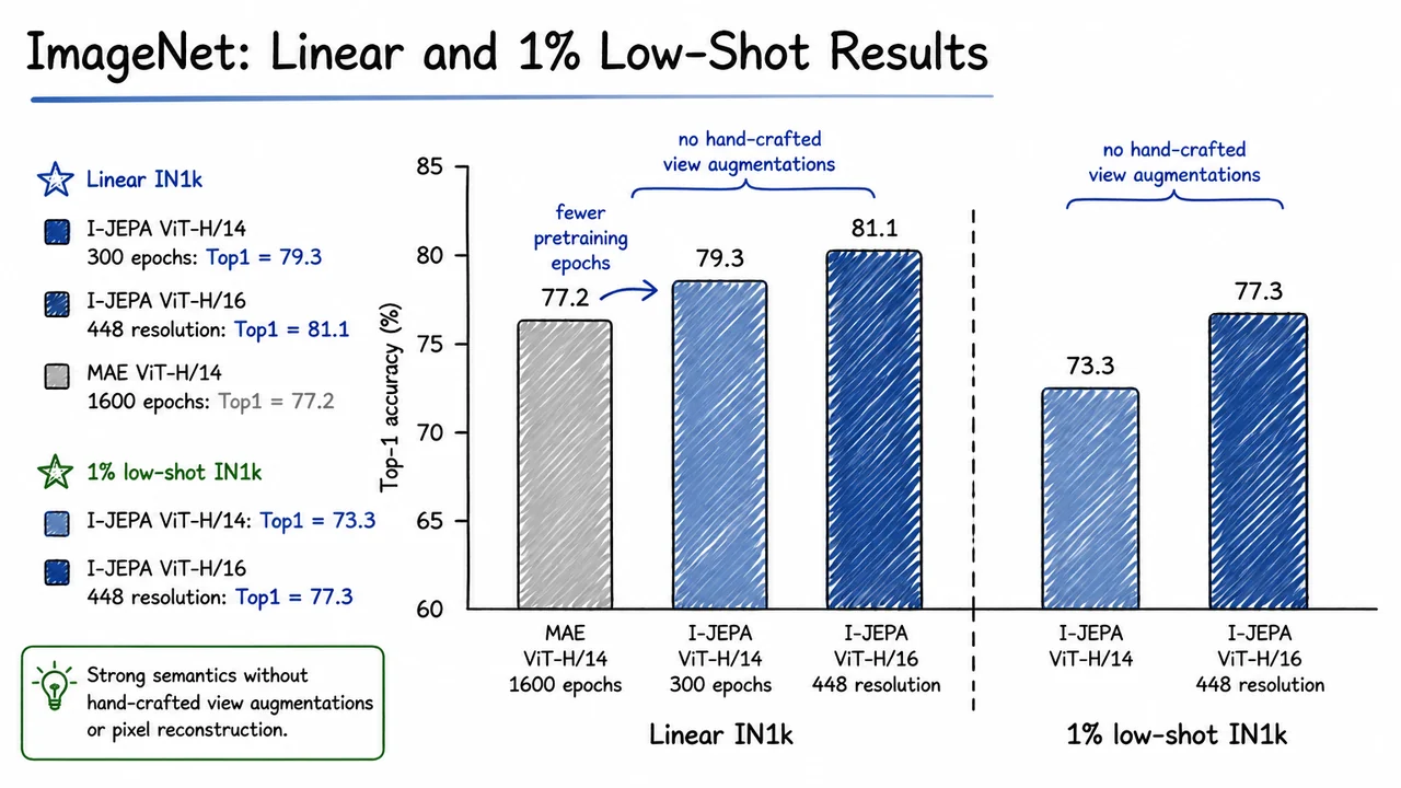
The ImageNet linear and 1% low-shot numbers are an important checkpoint, but they are not the whole story. A strong frozen linear probe tells us that I-JEPA has organized images into a representation space where category-relevant information is easy to extract. A strong low-shot result tells us something slightly stronger: the representation is not merely separable after seeing many labels, but label-efficient when supervision is scarce. That is exactly the kind of behavior we want from self-supervised pretraining.

Still, it is worth being careful about what these metrics actually certify. A linear classifier on top of a frozen encoder tests whether semantic class information is available in a relatively simple form. It does not fully tell us whether the model understands object parts, spatial relations, counting, geometry, or fine-grained local structure. A representation can be excellent for global image classification while being surprisingly weak at tasks that require preserving where things are or how many entities are present.

This distinction matters especially for I-JEPA because its training objective is not pixel reconstruction. Methods such as MAE are explicitly asked to recover missing patches in image space, so they are naturally pressured to preserve local texture, edges, and spatial detail. I-JEPA instead predicts target representations from a visible context. Its bet is that predicting in embedding space encourages the model to learn higher-level regularities rather than spend capacity on low-level photometric detail.

That design gives I-JEPA a plausible advantage for semantic transfer. By avoiding hand-crafted view augmentations and avoiding pixel-level reconstruction, it tries to learn invariances and abstractions from the structure of images themselves. But it also raises a natural concern: if the model is not reconstructing pixels, does it throw away too much local information? Does representation-space prediction preserve enough detail for tasks beyond image-level recognition?

This is where the empirical evaluation has to branch. The ImageNet results answer one question:

• Are the learned features useful for semantic categorization?
  The linear and low-shot results suggest yes.

But they leave open another question:

• Are the learned features useful for local or structured prediction?
  That requires separate probes, because global classification can hide weaknesses in spatial reasoning.

A useful way to think about this is that self-supervised representations are not judged by a single axis. There is a spectrum between semantic abstraction and local fidelity. Pixel reconstruction methods often sit closer to the local-fidelity side; contrastive or joint-embedding methods often emphasize semantic invariance; I-JEPA aims for a middle path, where the model predicts abstract representations but still receives enough spatially grounded masking pressure to learn about object layout and scene structure.

The key assumption is that the target encoder’s embeddings contain meaningful information about the missing region, and that the predictor cannot solve the task by relying only on trivial correlations. If the target representations collapse, the task becomes meaningless. If the context blocks are too informative or too close to the targets, the prediction task may become too easy. If the masking is too aggressive, the model may lack enough evidence to infer the target. The multi-block masking strategy is therefore not an implementation detail; it shapes the kind of information the representation must preserve.

The visual below can be read as a compact summary of this evaluation logic. The ImageNet probe sits as evidence that I-JEPA learns strong global semantics, while the next set of experiments asks whether those semantics come at the cost of local reasoning. In other words, the model has passed a high-level recognition test; now we want to know whether its representation still supports more structured questions about the image.

This transition is important because it prevents us from over-interpreting a single benchmark. Strong classification transfer is encouraging, but the more interesting claim is broader: I-JEPA’s representation-space prediction may learn features that are both semantically useful and spatially informative. The next local prediction tasks—such as counting and depth—are designed to probe exactly that claim.

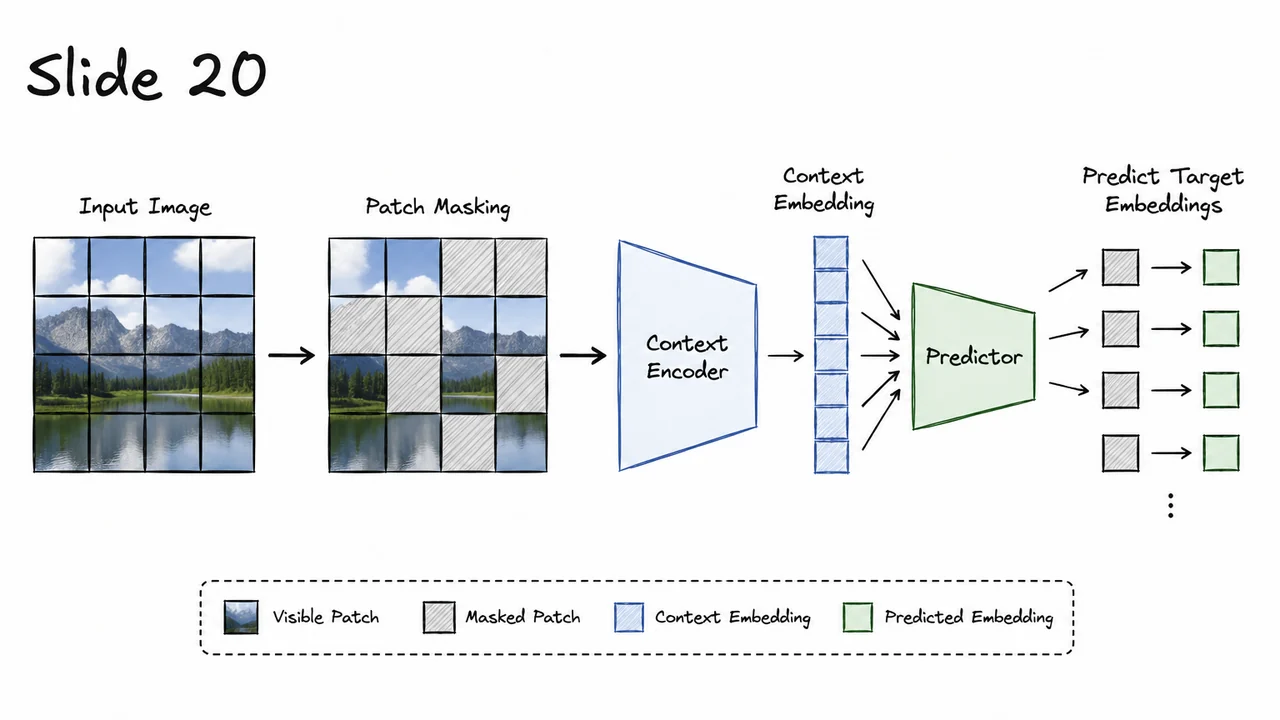
A useful way to evaluate a self-supervised representation is not only to ask whether it transfers to semantic classification, but also whether it still knows where things are and how many things are present. This matters because many successful representation-learning methods deliberately build invariances: two crops, color-jittered views, or transformed versions of an image are encouraged to map nearby in embedding space. That can be powerful for category-level recognition, but it also creates a tension. If two views are forced to agree even when one crop removes objects or changes the apparent layout, the representation may learn to discard information about count, pose, relative position, or depth-like spatial structure.

This is exactly the kind of failure mode I-JEPA is designed to avoid. Rather than constructing two heavily augmented views and demanding invariance between them, I-JEPA works inside a single image $I$. A context region $x$, corresponding to visible patches $B_x$, is used to predict the representations of held-out target blocks $B_i$. The target encoder produces representation-space targets $s_y(i)$, and the predictor learns to infer those missing block embeddings from the context representation. Abstractly, the training signal is not “make these two distorted views identical,” nor is it “reconstruct every missing pixel.” It is closer to:

$$\text{use visible image context } x \text{ to predict the semantic representation of hidden regions } s_y(i).$$

That distinction is subtle but important. Pixel reconstruction encourages the model to spend capacity on low-level detail: texture, color, edges, and other information that may not matter for downstream reasoning. Aggressive view invariance, on the other hand, can suppress local structure because the model is rewarded for ignoring differences between crops. I-JEPA tries to occupy the middle ground: it predicts in representation space, so it avoids pixel-level brittleness, while still using spatially localized masks inside one image, so the model must preserve enough layout information to make good predictions about missing regions.

The empirical question, then, is whether this design actually preserves local information in frozen features. Semantic transfer benchmarks tell us whether the representation is useful for recognizing object categories or scene-level concepts. But they do not fully test whether the representation contains information about numerosity or spatial arrangement. A model could classify an image well while being relatively insensitive to the exact number of objects or their relative depth ordering.

This is where the CLEVR local prediction tasks are useful probes. CLEVR is synthetic, controlled, and compositional, which makes it a good setting for asking targeted questions about what information is linearly accessible from frozen features. Two probes are especially relevant here:

• CLEVR Count asks whether the representation preserves object numerosity.
• CLEVR Dist asks whether the representation preserves spatial or depth-like layout.

These are not pretraining losses; they are downstream diagnostic tasks. The encoder is frozen, and a linear probe is trained on top. Strong performance therefore suggests that the relevant information is already organized in the representation, not learned from scratch by a powerful downstream head.

The reported I-JEPA ViT-H/14 results are:

$$\text{I-JEPA ViT-H/14: Count } 86.7,\qquad \text{Dist } 72.4$$

The Count result indicates that I-JEPA’s features retain information about how many objects are present. The Dist result is particularly interesting because spatial and depth-like relations are exactly the kind of information that can be weakened by crop-invariant training. If a model repeatedly sees crops where objects disappear, move out of frame, or appear in changed local contexts, it may learn that precise layout is not essential. I-JEPA’s single-image masked prediction objective avoids making those transformations into invariances.

Compared with view-invariance methods such as DINO and iBOT, I-JEPA performs especially well on the distance/layout probe. It also roughly matches MAE on CLEVR Dist, which is notable because MAE’s pixel-reconstruction objective is naturally spatial. The difference is that I-JEPA gets this locality without forcing the model to reconstruct raw pixels. In other words, it can retain local structure while still learning at a more semantic representation level.

The visual summary below condenses this comparison into the most relevant empirical pattern: I-JEPA is high on both local probes, with a particularly strong showing on the spatial-depth task. The orange bars mark the I-JEPA ViT-H/14 numbers, emphasizing that the representation-space prediction objective does not simply produce global semantic features; it also leaves local information linearly recoverable.

The key takeaway is not that counting and depth probes are the final goal, but that they expose an important tradeoff in self-supervised learning. A representation that becomes too invariant may lose precisely the details needed for structured visual reasoning. I-JEPA’s results suggest that predicting masked representation blocks from non-overlapping context regions can preserve that structure while avoiding both hand-crafted view invariance and pixel-level reconstruction as the central training target.

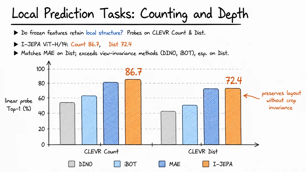
After seeing that I-JEPA’s representations carry useful local information for tasks like counting and depth, the next question is not just how good the representation is, but how much compute it costs to obtain. In self-supervised learning, this distinction matters enormously: a method that wins after hundreds of thousands of GPU-hours may be scientifically interesting, but a method that reaches comparable transfer quality with a much smaller compute budget changes what is practical to train, tune, and scale.

The empirical comparison here uses the same kind of downstream signal as before: ImageNet-1% Top-1 accuracy, a low-shot evaluation where only 1% of ImageNet labels are available for supervised adaptation. This is a useful probe because it rewards representations that are already semantically organized before labels are introduced. If a pretrained encoder has learned object-level structure, category-relevant invariances, and useful spatial abstractions, then a small amount of labeled data should be enough to extract good performance.

But now the x-axis changes: instead of asking only “what accuracy did the representation reach?”, we ask “what accuracy did it reach as a function of pretraining GPU hours?” That turns the evaluation into an efficiency study. In this framing, the ideal method lives in the upper-left region:

• high low-shot accuracy,
• low pretraining compute,
• favorable scaling behavior as model size grows.

This is where I-JEPA’s design choices become especially important. The method does not reconstruct pixels, and it does not rely on several heavily augmented views of the same image. Instead, it predicts missing-region representations from visible context representations. The context encoder $f_\theta$ processes only the visible context patches $B_x$, the target encoder $f_{\bar\theta}$ provides stop-gradient EMA targets, and the predictor $g_\phi$ is deliberately lightweight. So the training signal is semantic enough to avoid pixel-level waste, while the architecture avoids the high per-sample cost of multi-view contrastive-style pipelines.

This is the key computational contrast with MAE. MAE has a very efficient encoder path because it encodes only visible patches, but its target is still pixel reconstruction. I-JEPA’s representation targets make each iteration slightly more expensive—about 7% slower per iteration in the paper’s comparison—because target representations must be computed and predicted. However, this small per-iteration cost is more than offset by convergence speed: I-JEPA reaches strong performance in roughly $5\times$ fewer iterations. The important lesson is that iteration cost alone can be misleading. What matters is total compute to reach a given representation quality.

The contrast with iBOT is different. iBOT is a strong joint-embedding/self-distillation method, but it depends on multiple hand-crafted views of each image. Those extra crops and augmentations are not free: they increase the amount of image processing and encoder work per training example. I-JEPA’s single-view masked prediction setup avoids that multiplicative cost. This is one of the central motivations of the architecture: learn invariances and semantics through prediction in representation space, rather than by explicitly constructing many transformed views.

A subtle point is that I-JEPA is not simply “cheaper because it does less.” It is cheaper because it spends computation in a more targeted way. The model is not asked to reproduce every pixel of a masked patch, including low-level texture and color details that may be irrelevant for semantic transfer. It is also not asked to compare many augmented views just to discover invariances indirectly. Instead, the training problem asks: given surrounding context, can the predictor infer the latent representation of the missing region? That objective encourages abstraction while keeping the training loop relatively lean.

This also explains the striking scaling comparison reported in the paper: I-JEPA ViT-H/14 can use less compute than iBOT ViT-S/16 while maintaining strong low-shot performance. That is a surprising result because ViT-H is a much larger model family than ViT-S. Normally we expect larger models to dominate the compute budget. Here, however, the algorithmic structure matters enough that a larger I-JEPA model can still sit in a more favorable compute-performance region than a smaller model trained with a more expensive multi-view recipe.

The visual below compresses this argument into the geometry of a scatter plot. The y-axis is low-shot ImageNet-1% Top-1 accuracy; the x-axis is pretraining GPU hours. I-JEPA points occupy the efficient upper-left region, while MAE, data2vec, and iBOT appear farther to the right for comparable or weaker low-shot performance. The plot is qualitative in spirit: the important evidence is the relative placement of method families, not a single isolated number.

The annotations highlight the mechanisms behind that placement. The MAE comparison emphasizes the tradeoff between slightly slower iterations and far fewer total iterations. The iBOT comparison emphasizes the absence of multiple hand-crafted views. Together, these support the main takeaway: I-JEPA’s efficiency is not accidental; it follows from predicting semantic representations with a single-view masked architecture and a lightweight predictor.

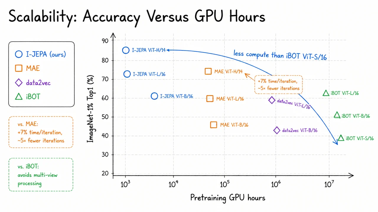
After looking at accuracy per unit of compute, the next question is what kind of scaling is actually responsible for the gains. In self-supervised vision, “scale” is an overloaded word: it can mean a larger encoder, more training steps, a higher-resolution input, or a broader pretraining distribution. These are not interchangeable. I-JEPA’s empirical story is especially interesting because its objective is designed to learn semantic predictive representations without relying on handcrafted augmentations or pixel reconstruction. That makes dataset diversity a particularly important stress test: if the representation is learning useful abstractions, exposing it to a wider visual world should improve transfer beyond the original pretraining domain.

The comparison here separates two axes. First, hold the backbone fixed and increase the pretraining dataset from $\mathrm{IN1k}$ to $\mathrm{IN22k}$. Second, hold the larger dataset fixed and increase the model from ViT-H/14 to ViT-G/16. These are both reasonable ways to spend more resources, but they probe different hypotheses:

• Data scaling hypothesis: broader visual diversity gives the model richer semantic and spatial regularities to predict.
• Model scaling hypothesis: a larger encoder has enough capacity to represent more refined structure, assuming the objective and data provide the right signal.
• Local precision caveat: more capacity may improve global category transfer while leaving fine-grained spatial reasoning unchanged.

This distinction matters because I-JEPA is not only evaluated on standard semantic transfer tasks such as CIFAR100, Places205, and iNaturalist18. The paper also tests more local or structured prediction settings, such as CLEVR counting and distance estimation. These tasks are useful because they ask whether the learned representation preserves information about where objects are and how they relate spatially, not merely what broad category is present. A representation can be excellent for classification while still discarding details needed for local geometry.

The fixed-backbone comparison is the cleanest evidence for the value of data diversity. Moving from ViT-H/14 pretrained on $\mathrm{IN1k}$ to ViT-H/14 pretrained on $\mathrm{IN22k}$ improves CIFAR100 from 87.5 to 89.5, improves iNaturalist18 from 47.6 to 50.5, and also improves CLEVR Count and CLEVR Distance from 86.7 to 88.6 and 72.4 to 75.0. Places205 is roughly stable, which is itself informative: the gain is not uniform across every benchmark, but the overall pattern is broad rather than confined to a single downstream setting.

That breadth is important. If $\mathrm{IN22k}$ only improved ImageNet-like classification, we might suspect simple label-space or domain overlap effects. But improvements on both semantic and local probes suggest that a more diverse pretraining distribution gives the joint-embedding predictor more useful invariances and more varied object configurations to model. In an architecture like I-JEPA, the model learns by predicting target-block representations from context-block representations. A richer dataset therefore changes the statistics of what must be predictable: object parts, layouts, scene context, species-level visual differences, and spatial arrangements all become more varied.

The model-scaling comparison is more subtle. Moving to ViT-G/16 on $\mathrm{IN22k}$ improves several semantic transfer metrics, which is consistent with the broader trend that large transformers can store and organize more abstract visual structure. But the local CLEVR-style probes do not automatically improve. This is a useful warning against a simplistic “bigger is always better” reading. Larger backbones increase capacity, but capacity alone does not guarantee that the representation allocates dimensions to the kind of precise spatial information a downstream probe needs.

One way to phrase the failure mode is that semantic compression and local precision can compete. A self-supervised encoder may learn features that are very stable under object appearance changes and viewpoint variation, which helps recognition. But those same features may become less sensitive to exact positions or distances unless the objective, architecture, masking strategy, and data distribution force that information to remain useful. I-JEPA’s multi-block prediction objective does encourage structured spatial understanding, but the empirical result says that simply increasing model size is not sufficient to keep improving it.

So the practical lesson is not “scale less,” but “scale the right axis for the representation you want.” If the goal is broad transfer, larger datasets and larger models can both help. If the goal includes spatially grounded or local reasoning, dataset diversity appears especially valuable, while model size should be treated as only one ingredient. This is an important point for interpreting self-supervised results: aggregate transfer numbers can hide whether the learned representation is becoming more semantic, more spatial, or merely more linearly separable on common benchmarks.

The visual below condenses this comparison into a compact table. The highlighted data-scaling row emphasizes the clean ViT-H/14 comparison between $\mathrm{IN1k}$ and $\mathrm{IN22k}$, where the gains appear across both semantic and local probes. The model-scaling row then separates the effect of increasing backbone size on the same broader dataset, making the caveat visible: semantic transfer improves, but local precision does not necessarily follow.

Read the two bottom callouts as the main empirical takeaway. Data diversity helps broadly because it changes the visual prediction problem the model sees during pretraining. Model scale is not the same as local precision because a larger encoder may learn more powerful global abstractions without automatically improving the spatial details needed for counting and distance judgments.

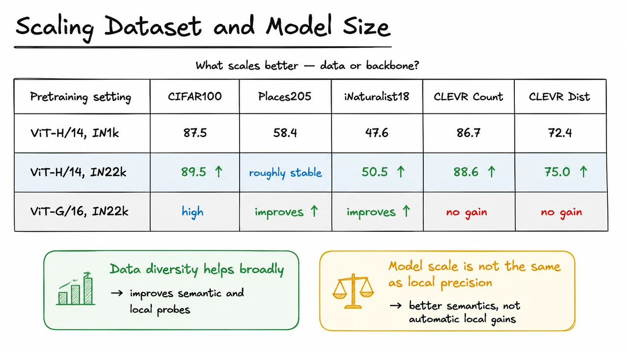
Scaling results tell us that I-JEPA becomes stronger as we increase data and model capacity, but they leave a deeper question unanswered: what kind of information is actually carried by the predictor’s output? If $\hat{s}_y(i)$ predicts the representation of a masked target block, does it contain something like a blurry reconstruction of the missing pixels, or does it encode a more abstract guess about the object part, pose, and scene layout?

This matters because I-JEPA’s central claim is not merely that representation-space prediction works, but that it encourages the model to focus on semantic regularities rather than pixel-level nuisances. The predictor is trained to map from a visible context representation $s_x$, together with mask-position information, into a predicted target representation:

$$\hat{s}_y(i)=g_\phi(s_x,\{m_j\}_{j\in B_i}).$$

Here $B_i$ denotes the target block, and the mask tokens $\{m_j\}_{j\in B_i}$ tell the predictor where the missing region is. Crucially, $\hat{s}_y(i)$ is not an RGB patch. It lives in representation space. So unlike a masked autoencoder decoder, the I-JEPA predictor is never directly asked to fill in texture, color, or exact contours. It only needs to produce something close to the target encoder’s embedding of that region.

But embeddings are hard to inspect directly. We can compare them with linear probes or downstream transfer, but those metrics do not tell us what visual attributes are present or absent in $\hat{s}_y(i)$. The RCDM visualization protocol is designed to answer exactly this kind of question: given a frozen representation, what aspects of the image can a decoder reliably recover from it?

The trick is subtle. Rather than training a decoder to reconstruct the image itself, the method perturbs an image with noise,

$$\hat{x}=x+\epsilon,$$

and trains a visualization decoder $h_\omega$ to reconstruct the noise $\epsilon$, conditioned on both the noisy image $\hat{x}$ and a representation. In the predictor-visualization setting, that representation is the average-pooled predicted target embedding $\hat{s}_y(i)$. The decoder is trained so that

$$h_\omega(\hat{x},\hat{s}_y(i))\approx \epsilon.$$

During this process, the pretrained I-JEPA components $f_\theta$ and $g_\phi$ are frozen. Only the visualization decoder $h_\omega$ learns. This distinction is important: the visualization is not changing what I-JEPA knows; it is only learning how to expose information already present in the predicted representation.

Why use noise reconstruction instead of direct image reconstruction? Because direct reconstruction can be misleading. A powerful decoder might hallucinate plausible pixels from image priors, or copy low-level information from its input. The RCDM setup probes the representation by asking which attributes remain stable across different noise samples. If the same target-region structure repeatedly appears even as the injected noise changes, that suggests the structure is encoded in $\hat{s}_y(i)$. If texture, precise background, or fine-grained color varies across samples, then those details are not strongly constrained by the representation.

So the interpretation is comparative rather than literal:

• Stable across samples $\Rightarrow$ likely represented in $\hat{s}_y(i)$.
• Variable across samples $\Rightarrow$ likely discarded, weakly represented, or left ambiguous.
• Coarse object part and pose stability $\Rightarrow$ evidence for semantic prediction.
• Texture/background variability $\Rightarrow$ evidence against pixel-level memorization.

This is exactly what the paper reports in its Figure 6 visualizations. When conditioning on the predictor output, the generated samples tend to preserve the broad identity of the missing target region: for example, the same object part appears in a consistent location and pose. But the exact surface pattern, local texture, and surrounding background often change. That is the behavior we would hope to see from a method whose objective is to predict abstract target-region representations, not to reconstruct the original pixels.

There is an important caveat, though. These visualizations are not a perfect microscope into the representation. They depend on the capacity and biases of the visualization decoder $h_\omega$, and “stable” does not always mean “explicitly linearly encoded.” The decoder may combine weak cues from $\hat{s}_y(i)$, the noisy input $\hat{x}$, and its own learned generative prior. Still, because $f_\theta$ and $g_\phi$ are frozen, and because variation across multiple noise draws can be inspected, the method gives a useful qualitative probe of what the predictor makes available.

The visual below compactly summarizes this probing setup. On the left, the usual I-JEPA machinery produces a predicted target representation from visible context and target-position mask tokens, with the pretrained encoder and predictor held fixed. On the right, a separately trained visualization decoder receives the noisy image and the predicted representation, then produces multiple reconstructions under different noise draws.

The key reading is the contrast between what stays fixed and what changes. The shared coarse silhouette or object-part pose corresponds to information that the predicted representation appears to carry. The changing textures and backgrounds correspond to information the predictor does not reliably specify. In that sense, the RCDM visualizations provide qualitative support for the broader empirical story: I-JEPA’s predictor learns to anticipate semantic content in representation space while leaving many low-level pixel details unresolved.

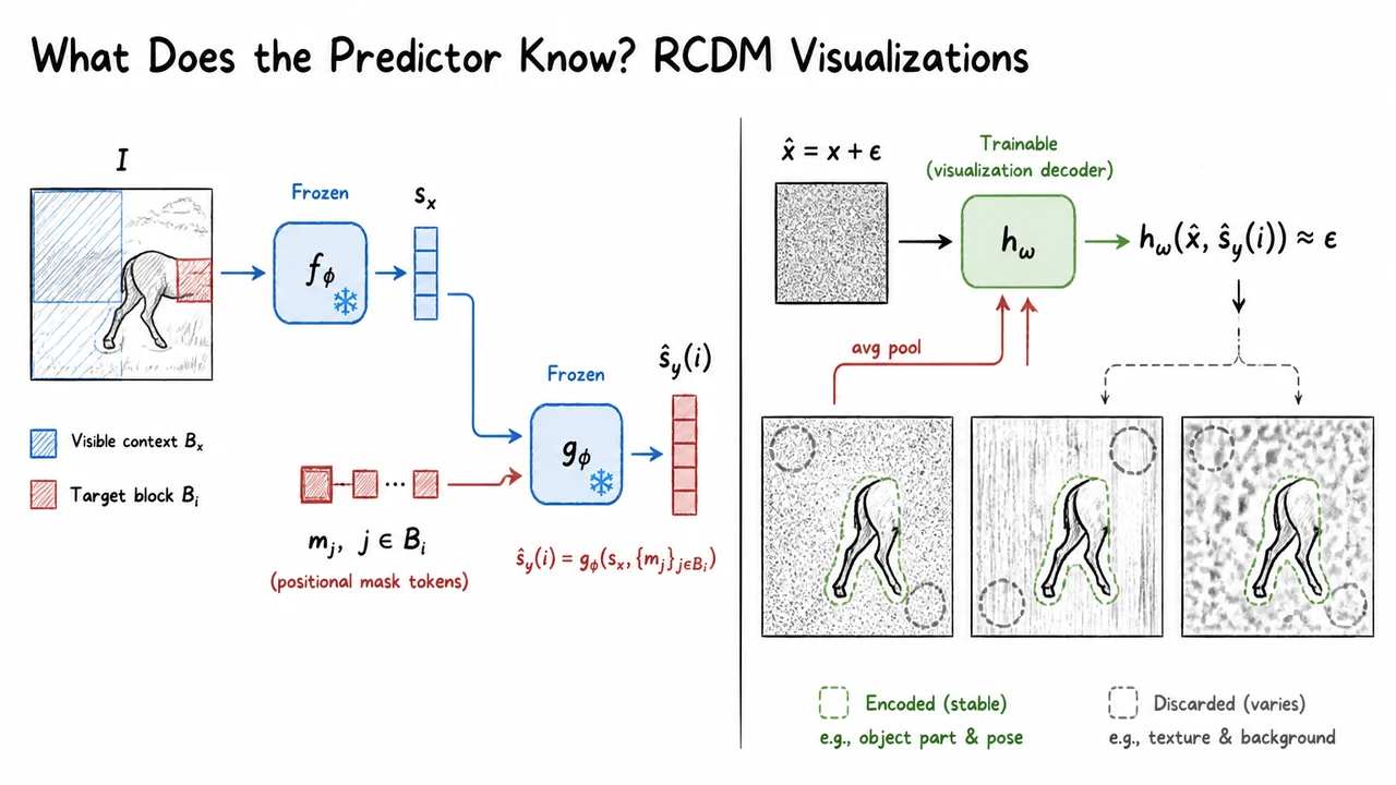
The RCDM visualizations gave us a qualitative clue about what the predictor seems to know: it is not merely copying texture or filling in low-level appearance, but often behaves as if it has learned something about object layout and semantic context. The natural next question is whether that behavior is actually tied to the central I-JEPA design choice. Is the model strong because of the masking recipe, the architecture scale, or optimization details—or because it predicts representations rather than pixels?

This ablation is one of the cleanest tests of JEPA’s core hypothesis. A pixel reconstruction objective asks the model to recover missing RGB values, which are extremely high-dimensional and contain many nuisance factors: lighting, texture, camera noise, local color statistics, and small spatial details. Those details are not useless, but they are often not the invariances we want for semantic transfer. If the goal is to learn a representation useful for recognition, segmentation, or downstream reasoning, then forcing the model to model every visible pixel can spend capacity on the wrong problem.

I-JEPA instead predicts targets in embedding space. The target encoder processes the image and produces a grid of latent vectors,

$$s_y = f_{\bar\theta}(y).$$

For a target block $B_i$, I-JEPA selects the corresponding subset of target representations,

$$s_y(i)=\{s^y_j:j\in B_i\}.$$

The predictor receives context information plus positional information for the target block and produces $\hat{s}_y(i)$. Training then minimizes a distance in representation space:

$$\mathcal{L} = \frac{1}{M} \sum_{i=1}^{M} D\bigl(\hat{s}_y(i),\operatorname{sg}(s_y(i))\bigr).$$

The stop-gradient matters: the target representation is treated as a stable prediction target, while the online context encoder and predictor learn to match it. In practice, the target encoder parameters $\bar\theta$ are updated by an exponential moving average of the online encoder, which prevents the target from changing too abruptly and helps avoid collapse.

The important subtlety is that $s_y$ is not just a compressed version of pixels. Because it is produced by a deep encoder, it can discard some low-level details and preserve more abstract information. This changes the nature of the prediction problem. Instead of asking, “what exact texture belongs in this missing patch?”, I-JEPA asks, “what representation should this region have, given the surrounding context?” That is a more semantic, less brittle task.

The empirical result is striking. When the paper compares representation targets against pixel targets, representation-space prediction is dramatically better on ImageNet-1k 1% linear evaluation: 66.9 top-1 versus 40.7, even though the pixel-target variant is trained longer, for 800 epochs instead of 500. That is not a small optimization artifact. It says that the choice of target space fundamentally changes what the model learns.

There is a second ablation that is just as revealing: where the masking happens in the target branch. The stronger version lets the target encoder see the full image first:

$$y \longrightarrow f_{\bar\theta}(y) = s_y,$$

and only then selects target blocks $B_i$ from the output representation grid. The weaker alternative masks the image before feeding it into the target encoder. That distinction may sound minor, but it changes the semantics of the target. If the target encoder receives the full image, its representation for a target block can be informed by global context and object-level structure. If the input is masked first, the target encoder is forced to represent an already-corrupted view, making the target less semantically complete.

The numbers again favor the representation-centric interpretation. Masking the output of $f_{\bar\theta}$ gives 67.3 top-1, while masking the input to $f_{\bar\theta}$ gives 56.1, under the same 300-epoch comparison. So the target branch is not merely a bookkeeping device for selecting patches. It is essential that the target encoder compute semantic representations from the unmasked full image before the model selects which blocks the predictor must match.

A useful way to summarize the lesson is:

• Pixel targets encourage reconstruction of appearance.
• Representation targets encourage prediction of semantic latent structure.
• Input masking in the target branch weakens the target because the target encoder sees a corrupted image.
• Output masking in the target branch preserves a rich full-image target and then asks the predictor to infer selected regions from context.

The visual below compactly organizes these two ablations. The table emphasizes that both comparisons point in the same direction: the best-performing variants are the ones that preserve I-JEPA’s core principle of predicting target-encoder embeddings rather than reconstructing pixels or corrupted inputs.

The small schematic is especially important conceptually. The preferred path is: full image $y$, target encoder $f_{\bar\theta}$, representation grid $s_y$, then block selection. The crossed-out alternative—masking before the target encoder—removes information too early. This is why the conclusion is stronger than “representations are convenient.” In I-JEPA, the target representation is the learning signal; it is the mechanism that turns masked prediction into semantic self-supervision.

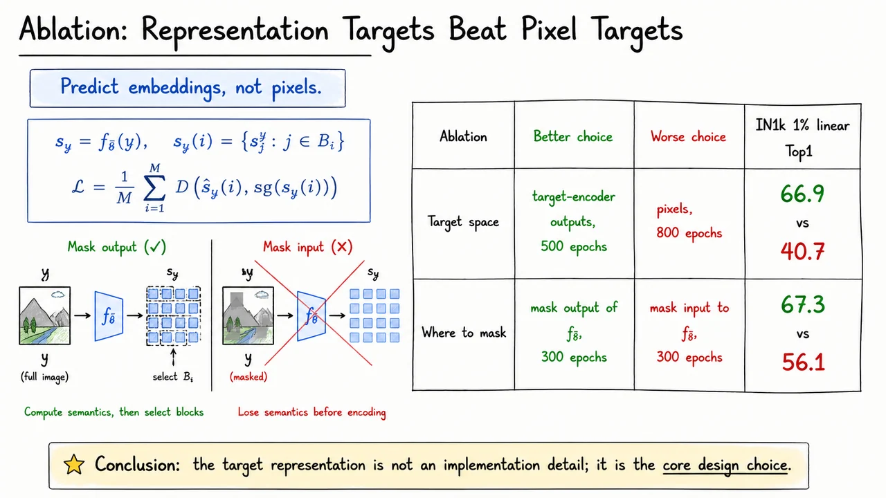
Having separated where I-JEPA predicts from what it predicts, there is one more ingredient that is easy to underestimate: the geometry of the missing regions. Once the target is a representation rather than pixels, the masking pattern is no longer just a corruption process borrowed from masked autoencoding. It defines the pretext task itself: what information the context is allowed to contain, what semantic uncertainty remains, and whether the predictor must reason about object-level structure or merely exploit local continuity.

In I-JEPA, the intended task is not “fill in arbitrary missing patches.” It is closer to: given a sufficiently informative visible region $B_x$, predict the representation of several non-overlapping target regions $B_1,\ldots,B_M$. The context encoder sees $B_x$, the target encoder produces embeddings for each $B_i$, and the predictor learns to map the context representation toward those target embeddings. Abstractly, for target block $B_i$, the training loss has the form

$$\mathcal{L} = \frac{1}{M} \sum_{i=1}^{M} \left\| q_\theta\!\left(f_\theta(x_{B_x}), B_i\right) - \operatorname{sg}\!\left(f_{\bar{\theta}}(x_{B_i})\right) \right\|_2^2,$$

where $f_\theta$ is the context encoder, $f_{\bar{\theta}}$ is the EMA target encoder, $q_\theta$ is the predictor, and $\operatorname{sg}(\cdot)$ stops gradients through the target branch. The block geometry determines how hard this objective is and what kind of abstraction it rewards.

A useful way to think about this is that the mask should remove information at the right semantic scale. If the target region is too small, predicting its representation may be possible from texture, color, or nearby patch statistics. If the target is too fragmented or randomly scattered, the model may learn a bag of local correspondences rather than coherent object-level prediction. But if the target block is large enough to contain meaningful parts of objects or scenes, then the context representation must encode more global structure: object identity, layout, pose, and relationships among visible and hidden regions.

This is why I-JEPA uses multi-block masking rather than a single masked area or a rasterized/random scheme. Multiple large target blocks increase the number of semantic prediction problems per image while preserving spatial coherence inside each target. The model is repeatedly asked: from this visible context, what should the representation of this absent semantic region be? That differs sharply from asking it to reconstruct pixels, and it also differs from asking it to predict many isolated missing patches with weak semantic identity.

The ablation numbers make this point unusually stark. For ViT-B/16 pretraining evaluated by ImageNet-1% linear probing, the intended setup—multi-block targets with a large context—reaches $54.2$ Top-1. By contrast, alternative masking schemes collapse badly: rasterized masking gives $15.5$, a single target block gives $20.2$, and random masking gives $17.6$. These are not small tuning effects. They suggest that I-JEPA’s success depends on constructing a prediction task whose ambiguity is semantic rather than merely local or noisy.

The appendix trends sharpen the interpretation. The best tested target scale is around

$$\rho \in (0.15, 0.2),$$

meaning each target block should cover a substantial, but not overwhelming, fraction of the image. The context must also remain large enough to support meaningful inference. Reducing the context scale from

$$\rho \in (0.85,1.0) \quad \text{to} \quad \rho \in (0.40,1.0)$$

drops performance from

$$\mathrm{Top1}=54.2 \quad \text{to} \quad \mathrm{Top1}=31.2.$$

That drop is intuitive: if the context is too impoverished, the prediction problem becomes underdetermined in a bad way. The predictor cannot infer semantic content from almost nothing, so the representation-learning signal becomes noisy or weak.

Target frequency is just as decisive. Increasing the number of target blocks from one to four changes the result from

$$M=1 \Rightarrow \mathrm{Top1}=9.0, \qquad M=4 \Rightarrow \mathrm{Top1}=54.2.$$

This is a dramatic reminder that the model needs many coherent prediction targets per image. A single block may provide too sparse a training signal, or may let the model overfit to narrow spatial shortcuts. Multiple blocks force the same context representation to support predictions about several missing semantic regions, encouraging a richer and more distributed image understanding.

The practical rule is therefore simple but important: predict several large semantic target blocks from a sufficiently informative, non-overlapping context. Multi-block masking is not decorative augmentation; it is part of the definition of the self-supervised task. If representation-space prediction tells the model not to waste capacity on pixels, then multi-block masking tells it which semantic abstractions are worth learning.

The visual below condenses this ablation into two pieces of evidence. The table contrasts masking strategies directly, highlighting that the multi-block, large-context recipe is the only one among the tested variants that produces strong ImageNet-1% transfer. The side callouts summarize the appendix findings: target blocks should be large enough, context should remain informative, and increasing the number of target blocks can transform a nearly failed objective into a strong one.

Read the figure as a warning against treating masking as an implementation detail. In I-JEPA, mask geometry controls the difficulty, ambiguity, and semantic content of the prediction problem. The empirical result is that the right geometry creates a useful representation-learning signal; the wrong geometry leaves the architecture and loss largely intact, but removes much of the learning value.

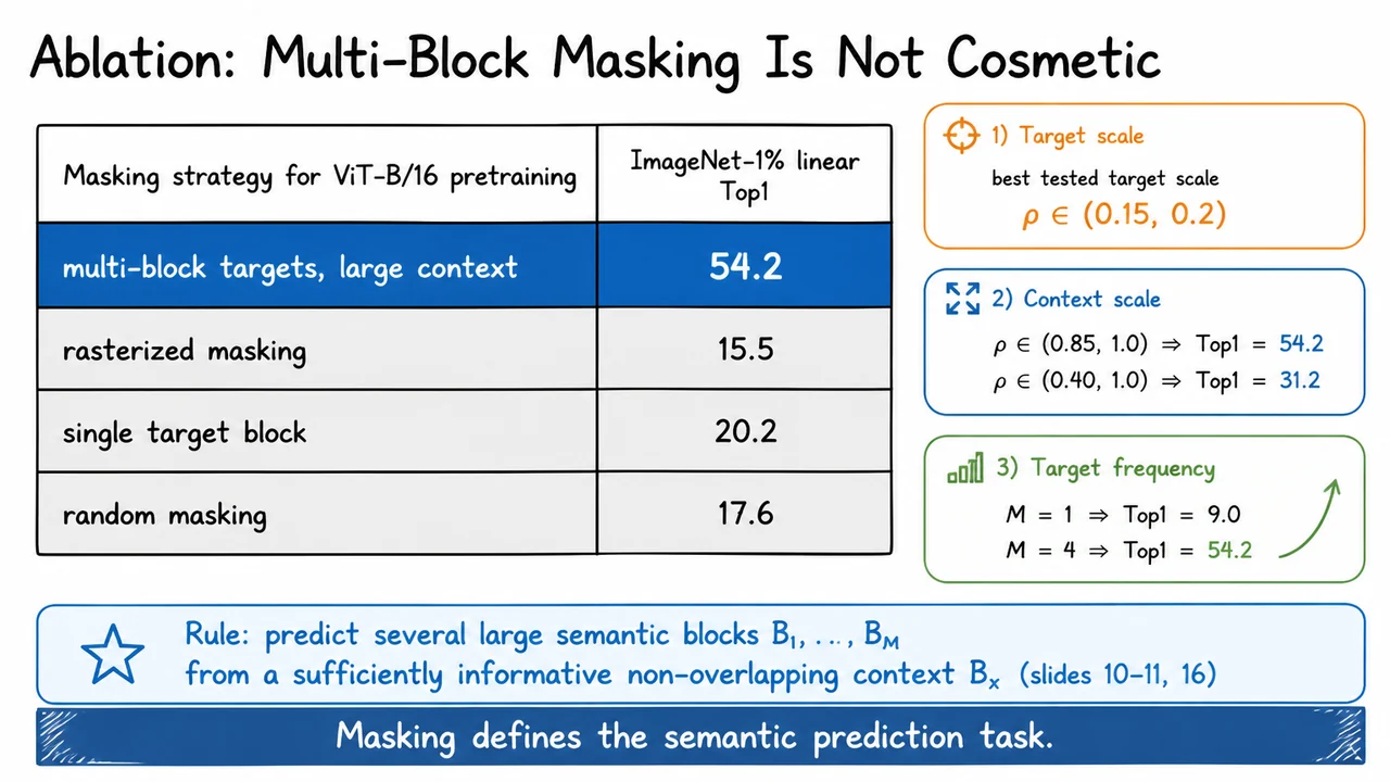
The masking ablation makes one point very clearly: I-JEPA’s prediction task is not just “hide some patches and regress something.” The geometry of what is hidden changes the kind of structure the model must infer. But once that structure is in place, there is still a second, more practical question: how much of the final result comes from the conceptual design, and how much comes from seemingly mundane choices like predictor size, bottleneck width, and weight decay?

This matters because I-JEPA’s predictor $g_\phi$ occupies an interesting role. It is not the encoder whose representations we ultimately want to transfer downstream, and it is not a pixel decoder that reconstructs low-level image content. Instead, it is a task-specific module trained to map a visible-context representation $s_x$, together with target-location information, into predicted target representations:

$$\hat{s}_y(i)=g_\phi\left(s_x,\{m_j\}_{j\in B_i}\right).$$

The target $s_y(i)$ is produced by the EMA target encoder, while $\hat{s}_y(i)$ is produced by the online context encoder plus the predictor. So the predictor is the place where the model can spend computation to solve the pretext task without forcing the context encoder itself to directly memorize every detail needed for prediction.

That separation is subtle but important. If $g_\phi$ is too weak, the training objective may become artificially hard: the context representation has to compensate for the predictor’s lack of capacity, and useful semantic information may not be extracted cleanly. If $g_\phi$ is too strong, one might worry about the opposite failure mode: the predictor could absorb too much of the pretext-task burden, allowing the context encoder to learn less transferable features. In practice, I-JEPA’s ablations suggest that predictor capacity does matter, but not in a way that overturns the main representation-space prediction principle.

The depth ablation is a good example. For a ViT-L/16 model trained for 500 epochs, a 12-layer predictor outperforms a 6-layer predictor, with reported linear evaluation accuracy improving from $64.0$ to $66.9$ Top-1. That is a meaningful difference. It says the predictor is not a disposable attachment; it needs enough expressivity to transform global context information and positional mask tokens into plausible target-block embeddings.

Width also matters, but again in a nuanced way. The paper reports that using a narrower 384-channel bottleneck can outperform a wider 1024-channel predictor in the IN1k 1% fine-tuning setting, with $70.7$ versus $68.4$. This is a useful reminder that “more capacity” is not always synonymous with “better representation learning.” A bottleneck can act as a regularizer: it may prevent the predictor from solving the objective through overly flexible transformations that do not require the context encoder to organize information in a broadly useful way.

Optimization choices show the same pattern. I-JEPA uses a weight-decay schedule that increases over training,

$$\lambda_t: 0.04 \rightarrow 0.4,$$

and this improves linear Top-1 performance compared with a fixed $0.05$ setting. But the fixed lower decay can sometimes help in low-label fine-tuning, such as the 1% ImageNet setting. That kind of result is not unusual in self-supervised learning: linear probing and fine-tuning do not always reward exactly the same representation geometry. Linear probing favors features that are already linearly separable; fine-tuning can benefit from features that remain more adaptable.

The broader lesson is that these choices are real levers, not cosmetic details. Predictor depth changes the solvability of the representation prediction task. Predictor width changes the balance between expressivity and regularization. Weight decay changes how strongly the model is pushed toward simpler parameter configurations over the course of pretraining. Any serious implementation of I-JEPA has to treat these as part of the training recipe, not as arbitrary defaults.

At the same time, these ablations refine the method rather than define it. The central idea remains: predict masked target-block representations from visible context in embedding space, rather than reconstructing pixels or relying on hand-crafted view augmentations. The engineering choices determine how efficiently and robustly that idea is realized, but they do not change the nature of the objective.

The accompanying visual compactly summarizes this distinction. The ablation table groups the evidence into three axes—predictor depth, predictor width, and weight decay—so the numbers can be read as practical sensitivities around a fixed JEPA loop. The small predictor schematic links those sensitivities back to $g_\phi$, emphasizing that the ablated component is the mechanism used to perform representation-space prediction, not a replacement for the principle itself.

The final callout is the key interpretation: tuning matters, but the conceptual gain is representation-space prediction. I-JEPA is not successful merely because of a particular predictor depth or decay schedule; those choices improve downstream results by making the core pretraining task work better.

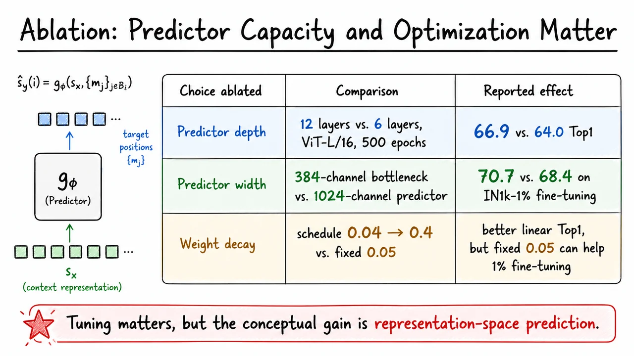
After seeing that predictor capacity and optimization details materially change the outcome, it is worth stepping back from the individual ablations and asking what the evidence really establishes. I-JEPA is not just “MAE in feature space,” nor is it simply another invariance-based joint-embedding method with fewer augmentations. Its central bet is more specific: learn semantic image representations by predicting missing regions in representation space, using spatial context and target blocks from the same image, while avoiding both hand-designed view transformations and low-level pixel reconstruction.

The strongest result is that this bet largely works. I-JEPA keeps the appealing abstraction of joint-embedding learning—compare representations, not pixels—while changing the source of supervision. Instead of constructing two augmented views and forcing their embeddings to match, it constructs a context region and one or more target regions, then trains a predictor to infer the target representation from the context representation. In simplified form, the training signal is

$$\mathcal{L} = \sum_i \left\| q_\phi\!\left(f_\theta(x_{\text{context}}), B_i\right) - \operatorname{sg}\!\left(f_{\bar\theta}(x_{B_i})\right) \right\|_2^2,$$

where $f_\theta$ is the online encoder, $f_{\bar\theta}$ is the EMA target encoder, $q_\phi$ is the predictor, $B_i$ indexes a target block, and $\operatorname{sg}(\cdot)$ blocks gradients into the target branch. The important philosophical move is that the model is not asked to reconstruct texture, color, or exact pixels. It is asked to predict a representation of what should be present in a missing spatial region.

That distinction explains several empirical strengths. First, I-JEPA performs well under frozen evaluation: ImageNet linear probing, low-shot learning, and transfer benchmarks suggest that the learned features are semantically useful rather than merely good at filling in local appearance. Second, the method does not appear to discard all local information. Because the prediction task is spatial and block-based, it still preserves enough structure for tasks such as counting and depth estimation to remain competitive. Third, the compute story is favorable. Although an I-JEPA iteration may be somewhat more expensive than pixel-masked modeling, the method can converge in far fewer epochs, which changes the practical cost-benefit calculation.

At the same time, the evidence does not make I-JEPA a clean theoretical resolution of self-supervised learning. The most delicate issue is collapse avoidance. In principle, joint-embedding losses can admit degenerate solutions: if every input maps to the same vector, prediction becomes trivially easy. I-JEPA avoids this in practice through a combination of design choices: an EMA target encoder, a stop-gradient target branch, predictor asymmetry, masking geometry, and optimization details. These are effective ingredients, but they are still partly empirical. We can explain why they are plausible, but we do not yet have a complete theory saying exactly when collapse is impossible.

There is also a nuanced comparison with generative masked modeling. I-JEPA often reaches strong representations with much less training, but it does not strictly dominate MAE on every metric. A useful anchor is the high-resolution fine-tuning comparison:

$$\mathrm{Top1}=87.1\%\ \text{(I-JEPA ViT-H/16 at 448, 300 epochs)} < 87.8\%\ \text{(MAE ViT-H/14 at 448, 1600 epochs)}.$$

This inequality should not be read as a failure of I-JEPA; it is more informative than that. It says that representation-space prediction can be dramatically more efficient and highly competitive, while still leaving room for pixel-reconstruction methods—especially very large, long-trained ones—to edge ahead under some full fine-tuning settings. The tradeoff is therefore not “semantic prediction good, reconstruction bad,” but rather a question of which target, at which granularity, under which compute budget.

The open questions follow naturally from this. I-JEPA depends on choices such as target block size $B_i$, number or frequency of target blocks $M$, context scale, and predictor capacity. These choices determine what kind of uncertainty the model must resolve. If targets are too small or too low-level, the task may reward texture-like prediction. If targets are too large or too ambiguous, the optimization problem may become unstable or overly reliant on dataset-level priors. Ideally, future methods would choose target granularity automatically, perhaps adapting it over training or across image regions.

Another open question is how far the JEPA principle extends beyond images. The representation-space prediction idea is broad: predict useful latent variables rather than raw observations. That sounds applicable to video, audio, robotics, language-grounded perception, and world modeling. But each domain changes the nature of “missing information.” In images, spatial blocks provide a convenient masking structure. In video, the missing content may involve time, causality, action, and object persistence. In robotics, the target representation may need to encode controllable aspects of the environment rather than merely predictable ones.

The visual below condenses this discussion into three buckets: what the empirical evidence has established, where the tradeoffs remain, and which design questions are still unresolved. The main point is not that I-JEPA is universally superior, but that it occupies a valuable position in the self-supervised learning landscape: it avoids hand-crafted view augmentations, avoids pixel-level reconstruction targets, and still learns strong transferable features.

It is especially useful to read the comparison as a map of maturity. The strengths are supported by the experiments we have just reviewed; the tradeoffs remind us that collapse prevention and final fine-tuning performance are not fully settled; and the open questions point toward the next generation of JEPA-style methods, where target selection and domain extension may become learned components rather than manually chosen design decisions.

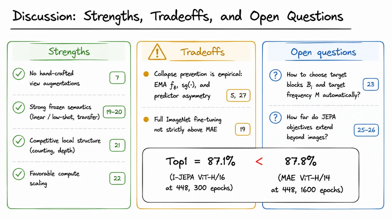
Stepping back from the strengths and tradeoffs, the cleanest way to organize the whole story is to ask a single question: what is the model asked to predict, and where is that prediction evaluated? Most self-supervised image methods can be understood as different answers to this question. They all exploit missing information, paired views, or both; they differ in whether the missing signal lives in pixel space, token space, or representation space, and in what prevents the learning problem from collapsing into a trivial solution.

The classical joint-embedding architecture view starts with two related inputs, say $x$ and $y$, and encodes them into representations $s_x$ and $s_y$. Learning is driven by a compatibility objective such as

$$D(s_x, s_y),$$

where $D$ rewards agreement between the two embeddings, often while additional mechanisms prevent all inputs from mapping to the same vector. This family includes many contrastive and non-contrastive invariance-based methods. Its strength is that it can learn highly semantic features: if two heavily augmented views of the same image must agree, the model is encouraged to ignore nuisance variation. But that is also its weakness. The definition of “same content” is largely hand-crafted through the augmentation pipeline. If the augmentations remove spatial layout, color, scale, or object details too aggressively, the representation may become invariant to information that downstream tasks still need.

At the other end are generative masked modeling approaches. These hide part of an image and ask the model to reconstruct the missing pixels or discrete visual tokens. In this case, the target is not another embedding $s_y$, but the input-level signal itself. This gives a very natural anti-collapse mechanism: predicting pixels cannot be solved by mapping every image to a constant representation. However, pixel reconstruction spends capacity on many details that are not necessarily semantic. Texture, color statistics, and high-frequency local structure can dominate the loss, especially when the reconstruction target is dense. These methods can be broad and robust, but their frozen representations are often less directly aligned with semantic transfer unless the model is large, trained long enough, or paired with a carefully designed decoder and tokenizer.

Hybrid methods combine these two instincts. They may use multiple augmented views while also predicting masked patches, or they may apply both view-level invariance losses and local reconstruction losses. This often works well because the objectives compensate for one another: invariance encourages semantic abstraction, while masked prediction preserves some spatial and local sensitivity. But hybrids also inherit costs from both sides. Multiple views increase compute, and mixed objectives introduce design complexity: which loss should dominate, which target should be reconstructed, how strong should augmentations be, and how should the model balance global semantics against local detail?

I-JEPA is best seen as a more surgical answer: keep the predictive structure of masked modeling, but move the prediction target into representation space. Instead of reconstructing pixels, the context encoder observes visible image regions and a predictor tries to infer the target encoder’s latent representations for masked blocks. The loss is applied to embeddings:

$$\mathcal{L} = \frac{1}{M} \sum_i \sum_{j\in B_i} \left\| \hat{s}^y_j - \operatorname{sg}(s^y_j) \right\|_2^2.$$

Here $B_i$ denotes a target block, $M$ is the number of target blocks, $\hat{s}^y_j$ is the predicted representation at target position $j$, and $\operatorname{sg}(s^y_j)$ is the stop-gradient target representation produced by the EMA target encoder. The stop-gradient is important: the target is treated as a stable quantity to predict, rather than something that can move freely to satisfy the predictor.

This design changes the nature of the learning problem. The model is not asked, “What exact pixels belong here?” It is asked, “What abstract representation should occupy this missing region, given the visible context and the region’s position?” The predictor receives mask tokens of the form

$$m_j = v + p_j,$$

where $v$ is a learned mask token and $p_j$ gives positional information. That positional grounding matters because I-JEPA is not merely predicting a bag of semantic concepts; it must infer representations at specific spatial locations. At the same time, because the target is a learned representation rather than raw pixels, the prediction can ignore many low-level details and focus on structure useful for recognition and transfer.

The remaining ingredient is asymmetry. I-JEPA uses a context encoder with ordinary trainable parameters $\theta$, and a target encoder with parameters $\bar{\theta}$ updated by exponential moving average:

$$\bar{\theta} \leftarrow \mu_t \bar{\theta} + (1-\mu_t)\theta.$$

This EMA target network provides a slowly moving prediction target. It is not a full contrastive mechanism, and it is not pixel reconstruction; it is a stabilizer that helps avoid representational collapse while allowing the target space itself to improve over training. Combined with large block masks, this creates the central inductive bias of I-JEPA: predict missing semantic regions from visible semantic context.

That is why the masking geometry is not a small implementation detail. Large target blocks force the model to reason beyond local texture continuation, while a large non-overlapping context block prevents the task from becoming a shortcut based on immediately adjacent pixels. The empirical ablations support this interpretation: I-JEPA works best when the missing regions are large enough to demand semantic inference, but still spatially grounded enough that the predictor must produce location-specific embeddings. The method’s efficiency also follows from the same design. Since it uses one image view rather than many augmented crops, and predicts in representation space rather than decoding pixels, it can reach strong transfer performance with fewer iterations than many heavier alternatives.

So the four families can be compared along a few decisive axes:

• What is given? Paired views, masked inputs, or one context view with masked target positions.
• What is predicted? Another embedding, raw pixels/tokens, mixed targets, or target-encoder representations.
• Where is the loss applied? In embedding space, input space, or both.
• What prevents trivial learning? Contrastive negatives, architectural asymmetry, reconstruction pressure, EMA targets, or combinations of these.
• What bias does the method encode? Augmentation invariance, signal reconstruction, hybrid consistency, or semantic block prediction.

The visual below condenses this comparison into a single summary table. Read it left to right: each row is not just a method category, but a different philosophy of self-supervision. JEA methods learn by making paired views compatible; generative masked models learn by reconstructing what was removed; hybrid methods combine view consistency with patch-level prediction; I-JEPA learns by predicting masked target representations from a spatially grounded context.

The green I-JEPA row and rule strip are the main endpoint of the lecture. They summarize the design recipe: mask the target encoder outputs, use multiple large target blocks, use a large non-overlapping context block, predict with positional mask tokens $m_j=v+p_j$, and update the target encoder by EMA. Put differently, I-JEPA’s contribution is not merely “masked image modeling without pixels.” It is a precise joint-embedding predictive architecture where abstract targets, block geometry, and EMA asymmetry work together to make the learned features semantic, spatially aware, and computationally efficient.

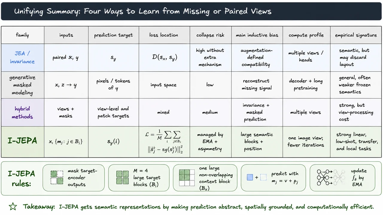
A useful place to begin is with the central tension in self-supervised vision: we want an encoder to learn from images without labels, but we do not want the pretraining task itself to quietly define the wrong notion of “understanding.” If the learned representation is later frozen and used for downstream tasks, then the pretraining signal has to encourage features that are semantic enough to transfer: object identity for classification, approximate numerosity for counting, geometry for depth, and many other properties that were never explicitly annotated during training.

Formally, we start with unlabeled images $I$ and train an encoder, often a Vision Transformer $f_\theta$, to produce representations that will later be reused. After pretraining, the encoder is commonly frozen, and a lightweight task-specific head is trained on top. This is why linear evaluation accuracy, often reported as $\mathrm{Top1}$, is such a useful diagnostic: if a linear classifier can extract category information from frozen features, then the representation already organizes images in a semantically meaningful way.

But the hard question is: what self-supervised prediction problem should force those semantics to emerge? Two dominant families of methods answer this differently. Joint-embedding methods often create two transformed “views” of the same image and train the model to make their representations agree. Masked image modeling methods often hide patches and ask the model to reconstruct missing pixels. Both strategies have been enormously influential, but both come with a possible mismatch between the pretraining objective and the representations we ultimately want.

The first risk is that hand-crafted view augmentations bake in assumptions. If we train a model to be invariant to random crops, color jitter, blur, or solarization, we are implicitly declaring that these transformations should not change semantic meaning. Often that is helpful. But it is not universally true. Cropping can remove the object of interest; color may matter for fine-grained recognition; geometric transformations may interfere with localization or depth. In other words, the augmentations are not neutral—they encode task-biased invariances.

The second risk is that pixel reconstruction can overemphasize low-level detail. If a model is rewarded for reconstructing RGB values, it may spend substantial capacity modeling texture, color continuity, and local statistics. Those details are real information, but they are not always the information we want a frozen encoder to prioritize. A pixel-level objective can succeed by becoming good at plausible image completion while still failing to build representations that are maximally useful for semantic transfer.

I-JEPA, the Image-based Joint-Embedding Predictive Architecture, takes a different route. Its claim is deceptively simple: predict missing information in representation space, not in pixel space, and do so without relying on pairs of hand-crafted augmented views. Instead of asking the model to reproduce the raw pixels of a hidden region, I-JEPA asks it to predict the representation that another encoder would assign to that region. The target is not “what exact colors go here?” but rather “what abstract representation should this missing part have, given the visible context?”

At a high level, we choose a visible context $x$ from an image $I$, with $x \subset I$. The context is encoded into a representation $s_x$. For a missing target block indexed by $i$, a predictor $g_\phi$ receives the context representation and information about the masked positions, represented by mask tokens $\{m_j : j \in B_i\}$. It then predicts a target representation:

$$x \subset I,\qquad \hat{s}_y(i)=g_\phi\bigl(s_x,\{m_j:j\in B_i\}\bigr), \qquad \hat{s}_y(i)\approx s_y(i).$$

The important phrase is $\hat{s}_y(i)\approx s_y(i)$. The model is not trained to make $\hat{y}$ look like a missing patch in RGB space. It is trained to make the predicted embedding $\hat{s}_y(i)$ match the target embedding $s_y(i)$. This places the learning signal at a more abstract level. If the target encoder produces semantic features, then the context encoder and predictor are pressured to infer semantic content from surrounding evidence.

This objective also changes what “prediction” means. Predicting pixels often rewards local realism: edges line up, colors continue, textures match. Predicting representations rewards compatibility with a learned feature space. That makes the task less about filling in every visual detail and more about inferring the latent structure that explains the image. The hope is that, by avoiding both augmentation-defined invariances and raw pixel reconstruction, the learned encoder becomes broadly useful rather than specialized to a pretext task’s quirks.

There are still subtle assumptions. I-JEPA assumes that the target representations are themselves meaningful enough to serve as learning signals, and that the masking strategy forces nontrivial contextual reasoning rather than shortcut prediction. If the hidden regions are too small or too locally predictable, the model may learn shallow continuity. If they are too large or disconnected from the context, prediction may become ambiguous. The design therefore depends on masking blocks at a scale where the model must use semantic context, not merely interpolate textures.

The visual summary below condenses this motivation into three pieces. On the left is the practical goal: train on unlabeled images, freeze the encoder, and transfer the representation to downstream tasks such as classification, counting, and depth prediction. In the middle are the two routes I-JEPA is trying to avoid as primary supervision signals: hand-crafted augmented views and pixel-level reconstruction.

On the right is the core alternative: use visible context $x$, encode it as $s_x$, combine it with mask-position information, and predict the missing block’s representation $\hat{s}_y(i)$ so that it matches $s_y(i)$. The headline empirical motivation is that this kind of representation-space prediction can scale to large ViTs—for example ViT-H/14 with patch size $P=14$ trained on $\mathrm{IN1k}$—while producing strong frozen-feature linear $\mathrm{Top1}$ performance with substantially less compute than several MAE- or iBOT-style baselines.

The previous point sets a high bar: we do not merely want features that make ImageNet linear probes happy; we want semantic image representations that remain useful when the downstream task changes. That is exactly where a first failure mode of popular view-invariance methods appears. Their success comes from making two transformed views of the same image agree, but the choice of transformations quietly defines what the model is allowed to forget.

In a typical joint-embedding method such as SimCLR, BYOL, DINO-style training, or related contrastive/non-contrastive approaches, we begin with an image $I$, sample two augmentations $t_1$ and $t_2$, and train an encoder so that

$$f(t_1(I)) \approx f(t_2(I)).$$

The objective is not literally saying “understand the whole image.” It is saying something more specific: produce similar representations after these hand-chosen perturbations. If the perturbations are semantically harmless, this is a powerful idea. A dog remains a dog under a crop, a color jitter, a blur, or a resize. For classification, these invariances are often exactly what we want.

But the hidden assumption is stronger than it first appears: whatever the augmentation removes or corrupts must be irrelevant to the representation. If a random crop cuts out half the scene, the model is still encouraged to map the crop close to another view of the original image. If color jitter removes appearance information, the representation is discouraged from depending too much on color. If blur destroys texture, or resizing changes apparent scale, the model is pushed toward features that survive those changes.

That pressure is not automatically wrong. In fact, it explains why view-invariance methods have been so effective for object category recognition. Classification often benefits from discarding nuisance variation:

• exact object position,
• background clutter,
• lighting and color shifts,
• small texture details,
• moderate changes in scale.

For a classifier, these details may be distractions. A robust “dogness” representation should not change much because the image was slightly blurred or the colors were altered.

The problem is that classification is only one downstream task. Many vision problems require precisely the information that standard augmentations treat as disposable. For object counting, a crop may remove one instance and change the correct answer. For depth estimation, resizing and cropping can distort cues about scale, perspective, and spatial relationships. For segmentation, weakening spatial layout is especially dangerous: the model must know not only what is present, but where each region and boundary lies. Color may also matter for materials, biological images, medical images, remote sensing, and fine-grained recognition.

So the issue is not simply “augmentations are bad.” The issue is that augmentations encode a task-biased invariance prior. They tell the representation which factors of variation should be ignored before we know which downstream task we care about. This is acceptable if the pretraining goal is aligned with classification-like transfer, but it becomes limiting when we want a more general visual representation.

This motivates one of I-JEPA’s central design choices: avoid relying on hand-crafted view augmentations as the main source of supervision. Instead of forcing agreement between aggressively transformed views, I-JEPA asks the model to predict missing information from visible context—but crucially, it predicts that information in representation space, not pixel space. The hope is to preserve semantic structure without requiring the designer to specify, through augmentations, which visual information should be invariant.

The visual below compresses this failure mode into a single causal chain. An image is transformed into multiple views through operations such as cropping, resizing, color jitter, and blur. The learning rule then forces the resulting representations to agree. That agreement is useful for classification, where invariance is often beneficial, but it can become harmful for tasks that depend on instance count, scale, appearance, or spatial layout.

The key takeaway is the warning in the middle: invariance means information has been discarded. Sometimes that discarded information is nuisance variation; sometimes it is the signal required by the next task. I-JEPA starts from this observation and asks whether self-supervised learning can avoid baking in so many manually chosen invariances while still learning high-level, transferable representations.

Avoiding hand-crafted augmentations removes one source of bias, but it does not automatically make the learning problem unbiased. A different family of self-supervised methods avoids explicit view design by corrupting the image itself and asking the model to fill in what is missing. This is the intuition behind masked image modeling: instead of saying “these two augmented views should match,” we say “given the visible part of the image, predict the hidden part.”

Formally, we start from an image signal $y$, then construct a corrupted or masked context $x$:

$$x = \text{masked or corrupted view of } y.$$

The model observes $x$, not the full image, and is trained to recover the missing content of $y$. In MAE-style methods, for example, a large fraction of image patches is removed, the encoder processes the visible patches, and a decoder reconstructs the missing pixels or patch-level visual tokens. This is attractive because it uses the image itself as supervision: no labels, no manually chosen positive pairs, no explicit color jitter or cropping policy that encodes assumptions about invariance.

But the choice of prediction target matters just as much as the choice of input corruption. If the target is raw pixels, then the loss function rewards whatever helps reduce pixel-level error. A typical reconstruction objective has the form

$$\mathcal{L}_{\text{pixel}} = \left\| \hat{y}_{\text{masked}} - y_{\text{masked}} \right\|^2,$$