A world model learns to predict future observations from past actions and sensory signals—in effect, an internal simulator that captures the causal structure of an environment. When built directly from high-dimensional pixels, such models can serve as the backbone for planning, sample-efficient reinforcement learning, and open-ended exploration. The allure is clear: rather than hand-crafting state abstractions, we learn a latent representation from raw images that distills the dynamics of the world into a compact code, then predict the next code using a predictor. This family of architectures, known as Joint-Embedding Predictive Architectures (JEPAs), avoids the need for a costly decoder back to pixel space by simply comparing against the encoding of the true next frame.
The elegance of JEPAs hides a potentially fatal flaw: representation collapse. Suppose we train the encoder and the predictor jointly with a mean-squared error loss . A trivial solution emerges—the encoder can map all images to the same constant vector, say . Then the predictor will learn to output regardless of the input , and the prediction loss drops to zero. The network has perfectly satisfied the objective, yet it has learned nothing about the environment’s dynamics; the latent representation is uninformative, and any downstream planning or probing task fails. This is the representation collapse problem, and it is not an edge case but rather the natural equilibrium of the naive objective, because the encoder and predictor can “collude” to ignore meaningful variations in the data.
Mathematically, if we denote the encoder output as a distribution over latent codes (or a deterministic point), the model can minimize the variance of under different inputs while also rendering the predictor’s output equally invariant. Even without resorting to constants, partial collapse where all lie on a low-dimensional manifold far simpler than the true state space is common: the encoder may merely preserve the easiest invariances (like brightness or average color) and discard fine-grained motion cues, again leading to trivial future prediction. Collapse is a fundamental identifiability failure: from the perspective of the prediction loss, many degenerate representations are equally optimal, and gradient-based optimization without explicit regularization will happily find one.
Intuition from classical self-supervised learning helps. In Siamese networks, collapse is prevented by comparing representations across different augmentations and employing a asymmetry (e.g., a stop-gradient with a momentum encoder) or by forcing the batch statistics to have high variance (e.g., VICReg). In BYOL, the target encoder’s exponential moving average coupled with a predictor network empirically avoids collapse without negative examples, yet the mechanism is subtle and can still drift toward low-diversity solutions if learning rates or EMA decay are poorly tuned. Contrastive methods (SimCLR, MoCo) avoid collapse by explicitly pushing apart representations of distinct inputs, but they require large batches of negative pairs and can be sensitive to the choice of similarity metric and temperature.
In the context of world models operating on sequential pixel data, these remedies face additional challenges. The temporal dimension introduces strong correlations—consecutive frames are nearly identical, making it harder to rely solely on batch-wise repulsion, because positives and negatives are not decorrelated as nicely as in static-image SSL. Adding a KL divergence to a prior, as in variational autoencoders, keeps the encoder from concentrating to a point, but can still permit collapse onto a small subset of the latent space if the prior is too permissive or the decoder is absent (as in JEPAs). Moreover, stop-gradient techniques decouple the encoder update from the predictor by using a slowly evolving target, but they introduce an architectural asymmetry that can slow down learning or cause the target to eventually catch up and collapse if hyperparameters are not carefully swept.
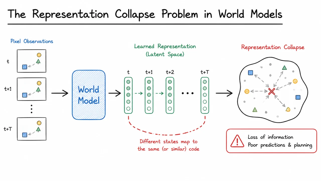
These observations underscore the need for a principled, provably anti-collapse regularizer that can be plugged into a fully end-to-end JEPA training loop without stop-gradients, without negative pairs, and without decoders. The upcoming sections will introduce Sketched-Isotropic-Gaussian Regularizer (SIGReg), which leverages the Cramér–Wold theorem to guarantee that the latent representations remain non-degenerate. But before we get there, it is essential to grasp just how insidious and catastrophic the collapse regime is. To that end, consider the visual below.
A schematic 2-D latent space illustrates the problem: several trajectories of true states—each corresponding to a distinct physical configuration—are drawn as colored sequences of connected points. On the left, before collapse, the encoder spreads these trajectories apart, preserving the topology of the dynamics. On the right, after collapse, all trajectories shrink into a dense ball and the predictor simply outputs the centroid of that ball for every action; the prediction error is zero, but the planner sees no meaningful distinction between a coffee cup tipping over and a robotic arm reaching for it. The collapse is complete, irreversible, and catastrophic for any world model that aims to support downstream reasoning. The regularizer we will derive directly penalizes such concentration, ensuring that the implicit geometry of the latent space remains rich enough to capture the environment’s causal structure.
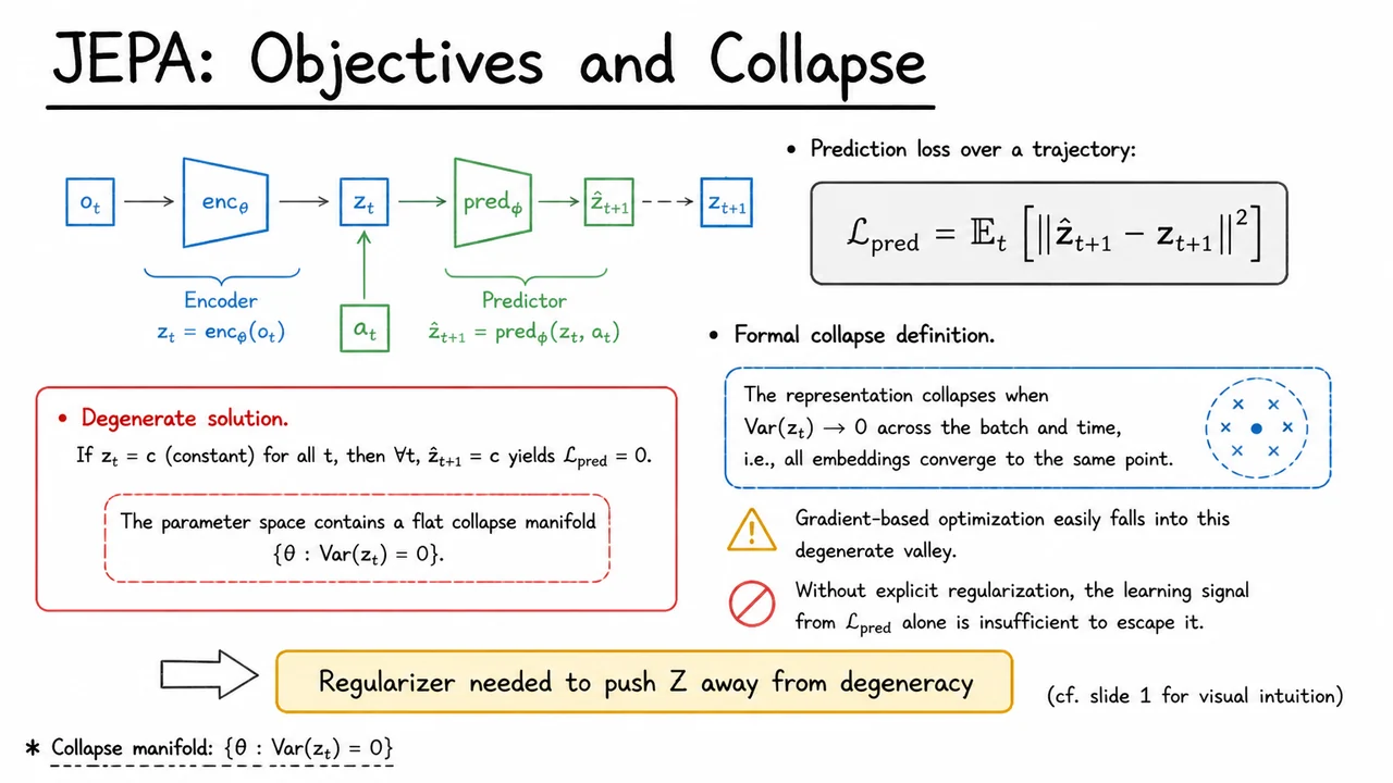
After establishing why representation collapse is a fundamental danger for any model that learns to predict its own representations, we now turn to the specific architecture class where this pathology is both most seductive and most damaging: Joint-Embedding Predictive Architectures, or JEPAs. These models are natural candidates for building world models from pixels because they avoid reconstructing high-dimensional observations and instead operate entirely in a learned latent space. An encoder maps each observation to a compact embedding . A separate predictor then takes the current latent state and an action to produce a prediction of the next latent state, . The learning objective is an expected squared error over a trajectory:
This loss function seems innocent enough—it simply asks the predictor to match the encoder’s output at the next time step. However, the joint optimization of encoder and predictor through this single mean‑squared error creates a deceptively flat loss landscape. Consider what happens if the encoder ignores the nuances of the input and collapses every observation to the same constant vector . Then for all , and the predictor can trivially output regardless of the action, achieving . The model has perfectly satisfied the training objective while discarding all information about the world.
This degenerate solution is not an isolated numerical accident; it forms an entire flat collapse manifold in parameter space. The manifold is defined by the condition across a batch or trajectory—meaning all embedding coordinates are identical and the representation has zero variance. Formally, the set contains infinitely many constant encoders that all yield the optimal loss. Because gradients of vanish on this set (the loss is already at its minimum), a gradient‑based optimizer that stumbles into this region will never leave. Worse, the manifold is attractive: near‑constant representations with tiny variance still give a very small loss, so the optimisation path can easily drift toward collapse without any repulsive force.
What makes JEPA’s collapse particularly insidious is that the learning signal from the prediction loss alone cannot detect that anything is wrong. The loss value itself is minimal and the gradients are negligible, so there is no inherent pressure to increase representation diversity. The problem is not that collapse is theoretically possible—it is that, in practice, stochastic gradient descent will reliably discover it unless explicit countermeasures are added. The encoder’s weights migrate toward a trivial mapping, the predictor becomes a constant function, and the world model loses all ability to distinguish states or plan actions.
The visual below summarises this architecture and the collapse trap in a single, compact diagram. It shows the encoder and predictor flow along with the mean‑squared prediction loss, and it illustrates the degenerate outcome where all latent vectors converge to an identical point, eliminating any variability. A red-outlined callout then underscores the essential conclusion: a principled regularizer is necessary to push the learned representation away from this degenerate valley. With that imperative in mind, we next examine prior strategies for preventing collapse and why they often fall short in the context of world model training.
In a plain Joint‑Embedding Predictive Architecture, the encoder and predictor can trivially drive the prediction loss to zero by collapsing all representations to a constant vector. Without an explicit incentive to preserve information, the latent space degenerates, making the model useless for downstream tasks such as planning or control. This catastrophic collapse is the central challenge that any JEPA‑based world model must overcome. The problem is not just theoretical: in practice, training a naive JEPA on pixel observations reliably produces dead latents within the first few iterations. So the question becomes: how can we prevent collapse while retaining the core benefits of end‑to‑end learning from raw sensory data?
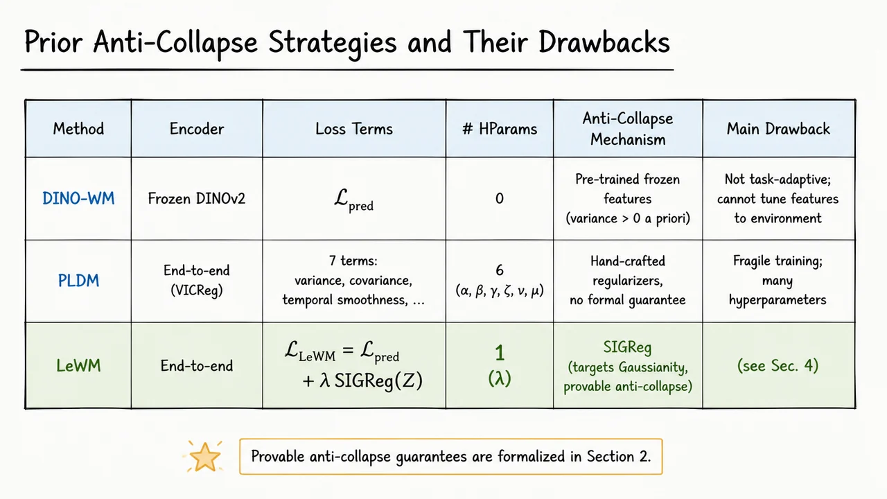
Prior work has explored two broad families of anti‑collapse strategies, each with distinct philosophical underpinnings. The first family avoids collapse by freezing the encoder. The logic is simple: if the encoder’s weights are fixed to a pre‑trained network that already yields informative, high‑variance representations, then collapse cannot occur because the encoder output is never updated toward a trivial solution. The DINO‑WM model exemplifies this route, using a frozen DINOv2 backbone to produce visual tokens and training only a lightweight predictor on top. The loss function is exactly the prediction error , with no auxiliary terms—zero extra hyperparameters. The anti‑collapse guarantee is baked into the prior: the pre‑trained features have non‑zero variance by construction, and the gradient never touches the encoder. This yields remarkably stable training and strong zero‑shot object‑centric representations. The glaring weakness, however, is that the encoder is not task‑adaptive. It cannot fine‑tune its features to the specific dynamics, textures, or regularities of the environment. In a world model meant to support physics‑aware planning, frozen features may miss subtle but critical relations—say, how friction depends on surface material—because they were never exposed to those correlations during pre‑training. The result is a ceiling on planning performance that no amount of predictor training can break.
The second family embraces end‑to‑end learning but tries to prevent collapse through a mix of hand‑crafted regularizers. The PLDM (Predictive Latent Dynamics Model) approach is representative: it pairs the JEPA prediction loss with a VICReg‑style cocktail of seven loss terms, including variance maximization, covariance de‑correlation, and temporal smoothness penalties. The full objective becomes a fragile sum of plus weighted regularizers, each controlled by its own coefficient—six hyperparameters in total (). The encoder is fully trainable, so the representation becomes adaptive to the environment. Yet the training is notoriously brittle: the interplay between the regularizers and the prediction loss can cause oscillations, mode‑dropping, or subtle forms of partial collapse where directions in latent space still vanish. Moreover, there is no formal guarantee that the ensemble of hand‑crafted terms actually prevents collapse; they merely nudge the representation toward certain desirable statistics. Tuning six hyperparameters for each new task becomes a barrier to widespread adoption, and the lack of theoretical grounding makes it hard to diagnose failures when they occur.
LeWM (LeWorldModel) proposes a third way: end‑to‑end training with a single, principled regularizer that carries a formal anti‑collapse guarantee. Its loss function is beautifully minimal: where the sketched‑isotropic‑Gaussian regularizer directly targets the distribution of latent codes. Drawing on the Cramér–Wold theorem, SIGReg ensures that the marginal distributions of all one‑dimensional projections of follow a standard normal law. Under mild conditions, this forces the full latent distribution toward an isotropic Gaussian, which has maximal entropy and strictly positive variance in every direction—hence collapse is impossible. The theorem provides a provable anti‑collapse guarantee without relying on frozen features or a heap of heuristic terms. Crucially, this guarantee holds while the encoder remains fully trainable, so the representation can adapt to the environment’s physics. Only a single penalty coefficient needs to be set, collapsing the hyperparameter count from six to one. This simplicity, combined with rigorous grounding, is the signature advantage of LeWM.
The following table consolidates the comparison. The visual contrasts DINO‑WM (frozen encoder, no hyperparameters, no adaptivity), PLDM (end‑to‑end, seven loss terms, six coefficients, fragile), and LeWM (end‑to‑end, one regularizer, one , provable anti‑collapse). The LeWM row is highlighted to draw attention to its unique combination: end‑to‑end adaptability and a single, theoretically justified regularizer. In the Loss Terms column, the table explicitly displays the massive difference in objective complexity, while the # HParams column dramatizes the reduction from six tunable knobs to just one. This side‑by‑side view makes it immediately clear why LeWM stands as a distinct advance: it captures the adaptability missing from DINO‑WM while dispensing with the fragile hyperparameter tuning of PLDM, all backed by a formal proof that collapse cannot occur. This foundation sets the stage for a detailed examination of LeWM’s architecture and the SIGReg mechanism, which we turn to next.
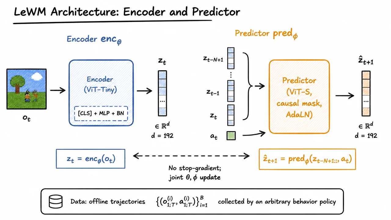
The stop-gradient trick, pioneered by BYOL and adopted by earlier JEPA variants, is a simple way to avoid representation collapse: the predictor receives a detached copy of the encoder’s output, so the encoder never sees gradients that would push it toward trivial solutions. But that convenience comes at a cost—the predictor must learn to compensate for an encoder whose parameters it never directly influences, and the two modules cannot truly co-adapt. LeWorldModel takes a different path. It proposes that we can train the encoder and predictor jointly, with gradients flowing freely through both networks, as long as we couple the training objective with a regularizer that provably prevents collapse. That regularizer (SIGReg) will be the focus of the next section; here we examine the architecture itself—a pair of Vision Transformers that maps pixel observations to latent states and predicts the next state conditioned on actions.
The encoder is a ViT-Tiny (approx. 6 M parameters) that takes a raw image observation and produces a compact latent embedding. After the transformer blocks, the final [CLS] token is projected by a single‑layer MLP with BatchNorm into a vector
This small latent dimension forces the encoder to compress the full visual scene into an efficient state representation, one that must be informative enough for the predictor to forecast the future. Notice that no stop‑gradient is applied here; the encoder’s parameters will receive gradient signals from the prediction loss.
The predictor is a larger transformer: ViT‑S (roughly 22 M parameters), but its architecture is tailored for temporal prediction. Given a history of the last latent embeddings and the current action , it outputs the predicted next latent To respect causality, the predictor uses causal masking inside its self‑attention layers: a token at position can only attend to tokens at positions in the history. This prevents information from the future from leaking backward, matching the autoregressive structure of a world model.
Action conditioning is implemented through Adaptive Layer Normalization (AdaLN). In every transformer block of the predictor, the pre‑normalization statistics are not learned scalars, but are instead computed as affine functions of the action . Concretely, the scale and shift parameters of the layer normalization become and , where are small linear projections. This design integrates the action deeply into the dynamics without adding extra tokens or altering the sequence length. It is both parameter‑efficient and empirically effective for learning continuous control dynamics from pixels.
The whole system is trained jointly, with a single prediction loss that compares the predicted next latent to the encoder’s output for the ground‑truth next observation , for example using the mean‑squared error or the cosine distance. Gradients update and simultaneously—no stop‑gradient is used anywhere in the forward pass. This is a deliberate choice: by allowing the predictor to shape the representation, the encoder can learn features that are not just descriptive of the current scene, but also predictive of the future. The risk, of course, is collapse: both networks could learn to output a constant vector. The upcoming SIGReg regularizer will eliminate that risk without interfering with the joint gradient flow.
The training data consists of offline trajectories collected by an arbitrary behavior policy. There is no online interaction with an environment during training; the world model is learned purely from prerecorded sequences. This makes the system amenable to large‑scale pre‑training on diverse datasets.
The accompanying diagram brings these pieces together into a single visual flow. It separates the left side—the encoder mapping an input image to a latent vector (blue block)—from the right side, where a stack of past latents plus the action feed into the orange predictor block to generate . A dashed bidirectional arrow across the entire diagram emphasizes the key design decision: no stop‑gradient; joint update of and . By glancing at this layout, one immediately sees the two‑stage decomposition (encode then predict) and the essential point that the model is trained end‑to‑end rather than being assembled from frozen pieces. It is a compact summary of the architecture we have just described, and it prepares the reader for the next step: understanding the regularizer that makes this joint training stable.
The encoder and predictor we built in the previous section map raw video frames into a sequence of latent vectors and forecast how those latents evolve over time. Without further constraints, this joint‑embedding predictive architecture faces a notorious enemy: representational collapse. The predictor can learn to ignore its inputs and emit a constant latent, or the encoder can produce the same vector regardless of the visual content. Many workarounds exist—stop‑gradient operations, contrastive losses, variance regularizers like VICReg—but they either break the differentiable flow needed for end‑to‑end planning or fail to prevent temporal degeneracies when stacked across many time steps. LeWorldModel takes a different route: it directly forces the marginal distribution of all latent vectors (across time and batch) to stay close to a standard isotropic Gaussian, . This soft constraint keeps the representations diverse, well‑conditioned, and easy for a dynamics model to predict, while entirely avoiding the need for negative samples or momentum encoders.
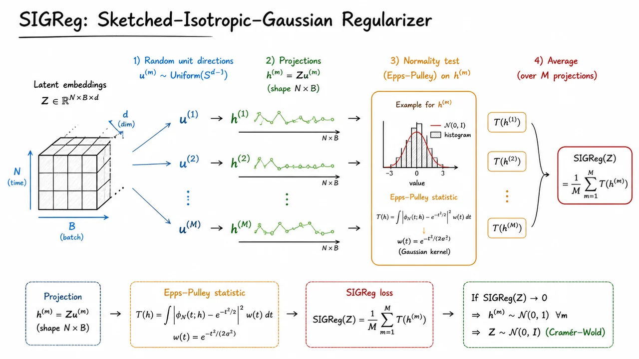
The question then becomes how to enforce in a high‑dimensional latent space that is typically hundreds of dimensions wide. Naïvely fitting a parametric density or using a kernel density estimator is computationally prohibitive and produces notoriously high‑variance gradients. A powerful theoretical shortcut comes from the Cramér–Wold theorem: a distribution is uniquely determined by the set of all its one‑dimensional projections. If we can guarantee that for every unit direction the scalar projection follows a standard normal distribution, then the joint distribution must be isotropic Gaussian. Translating this infinite set of constraints into a practical loss is the core idea behind SIGReg.
We approximate the full set of one‑dimensional marginals by sketching: draw random unit vectors independently of . For each direction we form the projected scalar set where is the tensor of all latent embeddings with axes (time steps , batch , dimension ). This reduces the high‑dimensional normality check to separate one‑dimensional tests. The name “sketched” comes from the fact that we use only a small, random sketch of the full projection space—typically a few hundred directions suffice to capture the essential structure.
For each projected sequence , we need a differentiable measure of how far its empirical distribution is from . The Epps–Pulley test provides exactly that. It compares the empirical characteristic function with the theoretical characteristic function of a standard normal, integrating the squared difference over a Gaussian kernel with fixed bandwidth : Crucially, this integral can be expressed in closed form as a double sum over all pairs of projected values, making it computationally tractable and directly differentiable with respect to (and hence ) via automatic differentiation. The statistic achieves its minimum of zero if and only if the sample comes from a standard normal distribution; larger values indicate deviation from Gaussianity.
Averaging across the random projections yields the SIGReg loss: This term is added to the main prediction loss, scaled by a hyper‑parameter , to form the total training objective . By construction, if we could drive to zero, then each projected marginal would be strictly standard normal, and by Cramér–Wold the full latent distribution would converge to . In practice, the regularizer never reaches zero; it merely provides a soft inductive bias that reliably prevents collapse and maintains a well‑spread latent space.
A few details are essential for stable training. The random directions are re‑sampled at every gradient step, so the regularization signal is always stochastic—this discourages the encoder from overfitting to a particular set of projections. The Epps–Pulley statistic is applied to the concatenation of latents from all time steps within a batch; this step‑wise treatment ensures that the regularizer fights not only static collapse (all latents equal) but also temporal collapse, where latents would otherwise drift toward a low‑dimensional manifold along the trajectory. Finally, the bandwidth of the weighting kernel is fixed, typically around 0.5–1.0, which controls the scale at which distributional discrepancies are penalized; it acts as a smoothness parameter that makes the normal approximation robust.
The visual below distills this computational pipeline into a diagrammatic flow that mirrors the derivation. On the left, a block represents the latent tensor with its three axes—time, batch, and feature dimension. A set of arrows, each labeled with a random unit vector , project onto scalar sequences , depicted as small one‑dimensional traces or histograms. On the right, for a chosen projection, we see its empirical histogram overlaid with the standard normal density, and a callout for the Epps–Pulley statistic . The average of all these values is then boxed as , emphasizing that the final regularizer is nothing but the sample mean over the random sketch. The color coding—blue for the projection directions, green for the projected values, and orange for the normality test—guides the eye from the high‑dimensional latent to the scalar goodness‑of‑fit quantities that together forge a practical, differentiable anti‑collapse guarantee.
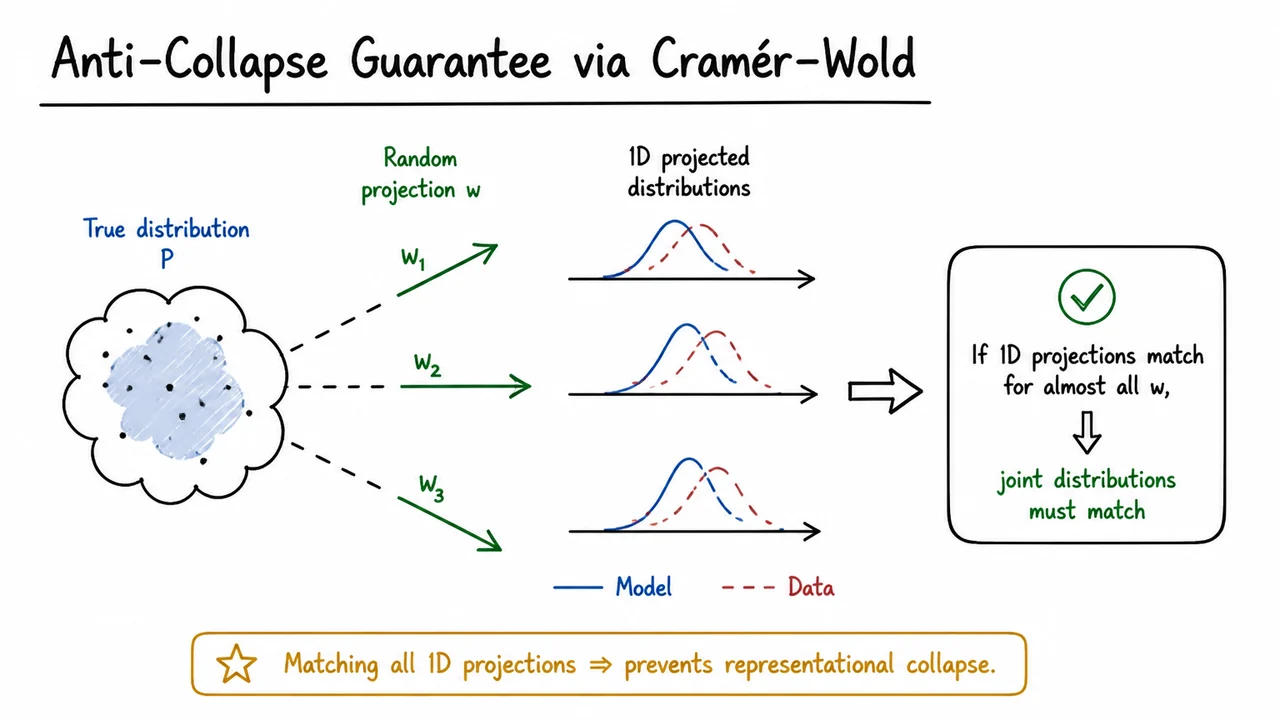
Having derived the Sketched-Isotropic-Gaussian Regularizer in the previous step, we now turn to a natural question: why is this regularization sufficient to prevent the representation collapse that plagues Joint-Embedding Predictive Architectures? In other words, can we formally guarantee that pushing the one-dimensional projections of the representation toward a standard Gaussian actually forces the full representation distribution to become non-collapsed? The answer lies in a classic result from probability theory—the Cramér–Wold theorem—which states that a multivariate distribution is uniquely determined by all its one-dimensional marginals. By applying this theorem, we obtain a rigorous anti-collapse guarantee for SIGReg.
Recall the central hazard in vanilla JEPAs: the target encoder and the predictor can jointly degenerate into trivial mappings. For example, the target encoder might output a constant vector, or the predictor might learn a fixed, low-complexity function that ignores the context. These failures manifest as a representation distribution that collapses—its effective rank drops, its variance shrinks in many directions, or it concentrates on a thin manifold. SIGReg counteracts this by encouraging the target encoder to produce latent vectors whose distribution resembles an isotropic Gaussian . But SIGReg does not enforce Gaussianity directly in the high-dimensional space; instead, it projects the representation onto a set of randomly chosen unit vectors (the sketches) and drives the distributions of those scalar projections toward a standard normal. The practical success of this approach rests on a profound insight: matching the distribution of all one-dimensional projections is equivalent to matching the full joint distribution.
The Cramér–Wold theorem provides the logical bridge. It says that two probability distributions over are identical if and only if, for every direction , the distribution of the linear projection is the same under both measures. Applied to our context: if every projection is forced to follow exactly the standard Gaussian , then the only consistent joint distribution is the multivariate standard normal . In the idealised world of infinite random sketches and infinite data, the SIGReg objective (for example, the sliced-Wasserstein distance between the representation distribution and ) would be zero exactly when the representation distribution equals the isotropic Gaussian. This gives a clean anti-collapse guarantee: the minimum of the regulariser corresponds uniquely to a non-collapsed, full-rank distribution, and any deviation from that distribution incurs a positive penalty. The representation is prevented from shrinking into a low-dimensional subspace because all directions must simultaneously exhibit unit variance and independent Gaussian behaviour.
It is important to appreciate the nuance that a regulariser matching only the first few moments of the projection distributions (e.g., mean 0 and variance 1) would not exploit the full force of the Cramér–Wold theorem; two different multivariate distributions can share identical univariate moments while differing in higher-order dependencies. SIGReg, by relying on distributional distances like the energy distance or maximum mean discrepancy (MMD) on the sketched scalars, compares the full distributions of the projections, not just their summary statistics. This makes the connection to the Cramér–Wold argument substantially more robust. In practice, we use a finite set of random directions—the sketch matrix—and compute the regulariser on mini-batches. While the theoretical guarantee now becomes approximate, the same intuition holds: as long as the number of sketches is large enough to “cover” the latent space sufficiently, minimizing the projection distribution discrepancy will drive the joint distribution toward an isotropic Gaussian, thereby guaranteeing high effective rank and diverse features.
Why does an isotropic Gaussian specifically prevent collapse? Because its covariance matrix is the identity matrix , meaning the representation has unit variance along every possible direction and no correlation between any two dimensions. This forces the encoder to use all available latent dimensions and to spread different aspects of the data across independent components, naturally combating the tendency to collapse to a constant or a narrow linear subspace. The regulariser thereby acts as a soft, geometry-aware constraint that preserves information throughput without manually tuning dimension-wise variance targets.
The visual below consolidates this guarantee into a single, glanceable diagram. On one side, a cloud of representation vectors is projected onto several randomly oriented lines (the sketched directions). For each line, the histogram or density of projected values is compared to a standard normal bell curve; the regulariser works to make them indistinguishable. A central annotation invoking Cramér–Wold points out that matching all these univariate marginals completely determines the multivariate distribution. As the regulariser takes effect, the initially irregular cloud is forced to expand into a perfectly spherical Gaussian ball, which in turn guarantees that the representation never collapses. The diagram therefore visually mirrors the proof: the series of 1-D marginals, each paired with , collectively reconstruct an isotropic high-dimensional Gaussian—the only possible joint distribution consistent with the constraint.
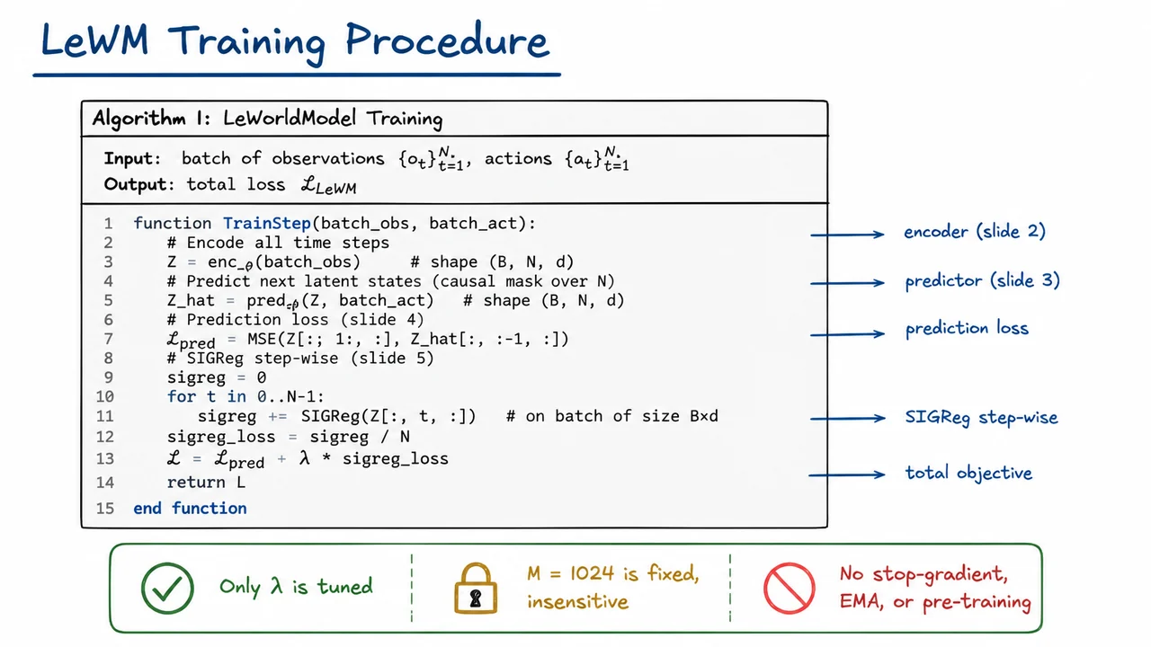
With the anti‑collapse guarantee of SIGReg established, we can assemble a training objective that is both simple and principled. The LeWorldModel training loop has exactly three ingredients: an encoder, a predictor, and the regularizer — and it requires only a single hyperparameter to balance them. There are no stop‑gradients, no exponential moving averages, no separate target networks, and no pre‑training stages. Everything is learned end‑to‑end from raw pixels in one continuous gradient flow.
The core idea is to impose a temporal consistency cost on the latent space while simultaneously preventing the representation from collapsing into a trivial constant. For a batch of sequences, each sequence of length with observations and actions , we first map every frame through the encoder , producing a latent tensor . The predictor then takes the full latent sequence up to time and the corresponding actions, and outputs predictions for the next latent state. Because the predictor operates causally — it cannot see future latents — the network must learn to anticipate how the world will evolve given an action.
The prediction loss is a straightforward mean‑squared error between the true next latent state and its predicted counterpart, averaged over all batch elements, all time steps (shifting by one), and all latent dimensions:
This objective alone would drive the latent states toward zero if the predictor could simply output zeros and still minimise the MSE when the encoder collapses. That is exactly the role of the step‑wise SIGReg term. At each time index , we apply on the batch of latent vectors of size . As derived, SIGReg uses a fixed set of random projection vectors and a student‑t tail index to penalise latent distributions that are not isotropic Gaussian, thereby maintaining a rich, non‑degenerate representation:
The averaged regularisation over the temporal dimension becomes . The final objective couples prediction and regularisation with a single scaling coefficient :
All hyperparameters except are effectively fixed — is large enough to be insensitive, and the student‑t degrees of freedom are chosen once based on the collapse‑prevention analysis. The training step is simply a forward pass through encoder and predictor, computation of the two loss components, and backpropagation of the weighted sum.
This design is deliberately minimal. The encoder and predictor are updated with the same learning rate; there is no gradient blocking between them. The regularizer operates only on the encoder outputs, not on the predictions, which neatly decouples the anti‑collapse mechanism from the predictive learning task. The causal masking inside the predictor ensures that the model learns a forward dynamics model that can later be unrolled during planning, without leaking future information.
The visual below condenses the full training algorithm into a compact pseudocode box, with side annotations that connect each line back to the earlier components: the encoder (slide 2), the predictor (slide 3), the prediction loss (slide 4), and the step‑wise SIGReg (slide 5). The highlighted call‑out at the bottom emphasises the key practical takeaway — only is tuned; is fixed — which underscores the method’s robustness and ease of adoption. By treating the training loop as a composable pipeline, the diagram makes evident how each theoretical piece slots into a working implementation, leaving no hidden engineering tricks to obscure the core ideas.
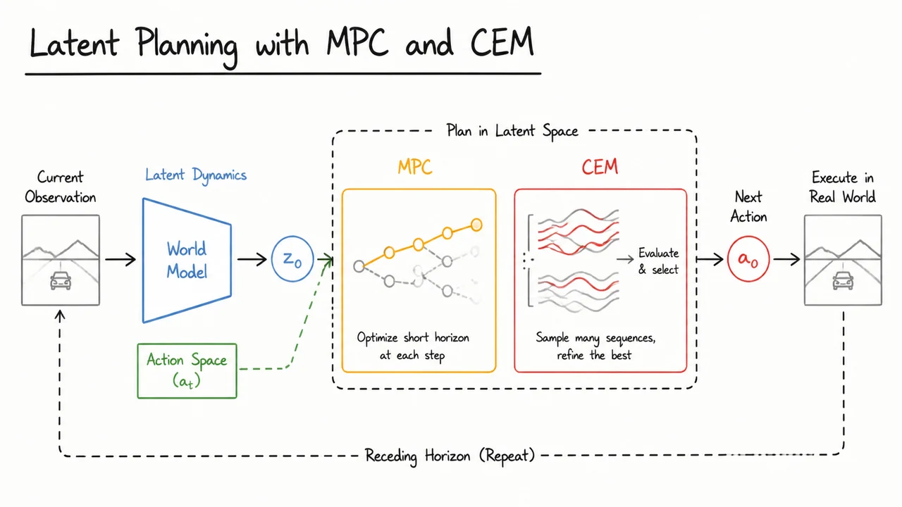
Having trained a stable latent world model that reliably maps pixel observations into a compact representation and predicts future latents without collapse, the next practical question is: how do we use this model to choose actions that achieve a goal? The answer in LeWorldModel is latent planning—specifically, a model predictive control (MPC) loop that optimizes action sequences entirely inside the latent space, paired with the cross‑entropy method (CEM) as a gradient‑free optimizer.
The core motivation is efficiency and coherence. Because the encoder compresses high‑dimensional images into a relatively low‑dimensional latent state , and the learned latent dynamics predicts from and an action , we can simulate many future trajectories without ever decoding back to pixels. This avoidance of high‑resolution generation dramatically reduces the computational cost per rollout, making it feasible to evaluate thousands of candidate action sequences online. Moreover, if the world model has been trained with the anti‑collapse regularizer (SIGReg), the latent rollouts stay well‑behaved over long horizons, so planning does not suffer from the explosive noise or mode drift that plagues unregularized JEPA‑style models. The planning problem then reduces to solving
where is a reward function defined directly on the latent state (either an additional learned head or a simple function of the latent coordinates), and is the finite planning horizon.
MPC is a natural fit for this setting. At each environment time step, the planner computes an optimal action sequence for the next steps, but only the first action is executed; then the whole process repeats given the new observation. This receding‑horizon loop adds a layer of feedback that helps correct for modelling errors, because the planner constantly incorporates fresh sensory evidence. However, the latent dynamics are typically non‑differentiable with respect to actions (especially when trained end‑to‑end with discrete action spaces or stochastic components), and the reward landscape can be highly non‑convex. Therefore a derivative‑free optimizer is required.
The cross‑entropy method (CEM) is employed as a black‑box optimizer for the action sequence. CEM iteratively refines a sampling distribution—usually a multivariate Gaussian over the sequence of actions—by repeatedly evaluating sampled sequences through the latent dynamics and reward model, then refitting the distribution to the top‑performing elite samples. Concretely, the planner maintains a mean vector and covariance matrix for the action sequence. In each CEM iteration:
This procedure works well even when the underlying dynamics are only approximately correct, because CEM does not rely on gradient signals through the world model; it merely requires a way to score candidate plans. At the same time, the compactness of the latent space keeps every rollout cheap—often thousands of rollouts can be evaluated in real time on a single GPU.
From a theoretical perspective, the success of this planning pipeline is tightly coupled to the stability guarantees of the world model. If the latent dynamics were prone to collapse—say, all future latents being mapped to a constant vector—then CEM would receive no meaningful reward variation and would be unable to distinguish good action sequences from bad ones. The Sketched‑Isotropic‑Gaussian regularizer ensures that the predictions preserve diversity and remain faithful to the true data distribution, so the rollouts remain informative for planning.
The visual below captures this loop in a single glance. It shows the pixel observation flowing into the encoder to produce the current latent state; from there, a CEM planner samples action sequences, passes them through the latent dynamics predictor to generate a batch of imagined latent trajectories, and scores each trajectory with a reward function. The elite samples are fed back to update the sampling distribution, and the final mean action is output to the environment. The diagram uses clean, hand‑drawn arrows and muted color accents to separate the planning cycle (in blue‑green tones) from the environment interaction (in amber), making the receding‑horizon, sample‑based nature of the approach immediately graspable. Together with the preceding stability analysis, it reinforces that latent planning with MPC and CEM is not merely a heuristic but a principled design choice enabled by a robust, collapse‑free world model.
The latent planning framework described earlier gives us an elegant way to reuse a frozen world model for control: given a start observation, encode it into a latent state , and then use model predictive control (MPC) to find an action sequence that minimizes the expected squared distance from the predicted terminal latent state to a goal latent state . The full planning objective is
where the expectation is over the stochastic latent dynamics learned by LeWorldModel. This objective implicitly defines a goal‑conditioned planner that never sees an explicit reward function—it simply attempts to make the latent future match the latent goal. The optimization is performed with a cross‑entropy method (CEM) that samples action sequences, propagates them through the learned dynamics, and iteratively refines the sampling distribution toward promising sequences. The whole procedure produces control policies purely from the model’s internal representation of the world, without any online interaction or online reinforcement learning.
What makes this setup particularly interesting to evaluate is that the planning performance directly reflects the quality of the learned latent space and the learned dynamics. If the representations are not temporally predictive, or if the dynamics model hallucinates unrealistic transitions, the optimizer will fail to reach the goal with any reasonable budget of CEM iterations. Conversely, a well‑regularized joint‑embedding architecture should produce a latent space where Euclidean distance to the goal embedding serves as a useful surrogate for task success, and where forward unrolling remains accurate over the planning horizon.
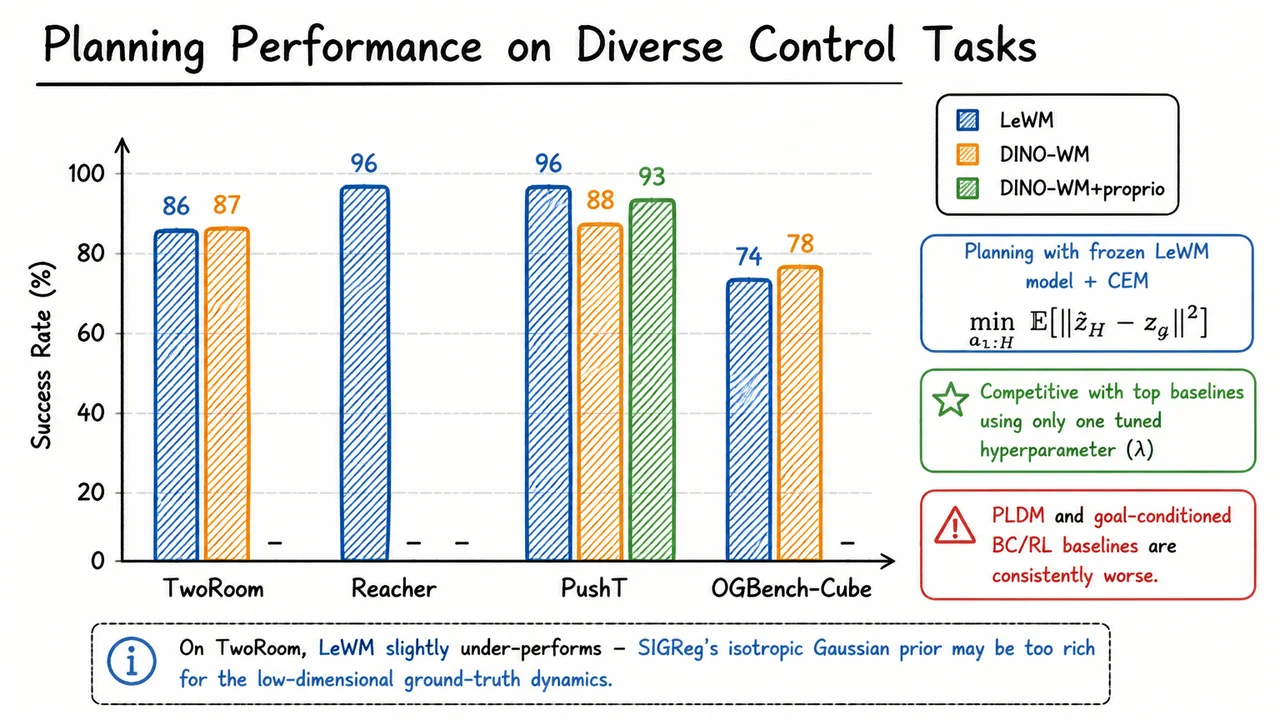
To understand the practical strengths and limitations of the LeWorldModel pipeline, we compare it against a range of strong baselines on four visual control tasks spanning different levels of difficulty: TwoRoom (point‑mass navigation around a wall), Reacher (robot arm reaching a target position), PushT (pushing a T‑shaped object into a desired pose), and OGBench‑Cube (a dexterous in‑hand cube rotation task). All tasks provide only pixel observations; the model has no direct access to proprioceptive information unless that channel is explicitly added. The evaluation metric is simple and unforgiving: a trial is counted as a success if the final state achieves the goal within a predefined tolerance, and we report the planning success rate (%) over many randomized goal–start pairs.
For comparison we include recent joint‑embedding baselines such as DINO‑WM (a world model built atop DINO pre‑trained features, fine‑tuned for planning) and its proprioceptive variant DINO‑WM+proprio, as well as standard offline goal‑conditioned behavioral cloning and offline RL methods (PLDM is a representative example). Crucially, LeWM uses a much simpler training objective than most competitors—a single joint‑embedding predictive loss regularized by SIGReg—and introduces only one hyperparameter that requires tuning per task: the regularizer coefficient . In contrast, many baselines rely on task‑specific reward engineering, expensive pre‑training recipes with large foundation models, or additional proprioceptive inputs.
The visual below consolidates the main findings as a grouped bar chart. Across the four tasks, LeWM achieves success rates that are competitive with the best‑performing baselines, and in several cases it sets a new high mark. On Reacher, LeWM scores 96 %, exceeding all non‑proprioceptive methods by a comfortable margin. On PushT, which is especially challenging because of the need to reason about object contact and geometry from pixels alone, LeWM reaches 96 % while DINO‑WM achieves 88 % without proprioception and 93 % with proprioception. Even on OGBench‑Cube, a task that demands precise high‑frequency manipulation, LeWM’s 74 % is only slightly behind DINO‑WM’s 78 %, despite DINO‑WM’s use of an additional visual pre‑training stage on large‑scale data. And critically, PLDM and the offline RL and behavioral cloning baselines are consistently outperformed, highlighting the advantage of a joint‑embedding model that learns its own state representation jointly with the dynamics, rather than using a fixed feature extractor or relying on an externally shaped reward.
The one notable shortfall occurs on TwoRoom, where LeWM attains 86 % versus DINO‑WM’s 87 %. This slight under‑performance reveals a thoughtful design choice: the SIGReg regularizer encourages the latent distribution over to approach an isotropic Gaussian. This is a deliberately rich prior that avoids representation collapse even in high‑dimensional sensory streams, but it can become a mild liability when the true latent dynamics are genuinely low‑dimensional. TwoRoom, a deterministic 2D navigation problem with a single obstacle, has an underlying state manifold that is essentially a 2D Euclidean subspace. An isotropic Gaussian prior spreads probability mass across many dimensions that the dynamics will never need, and the model consequently spends some capacity modeling harmless but useless stochasticity, slightly degrading planning accuracy. This matches the theoretical anti‑collapse guarantee from the Cramér–Wold theorem: SIGReg always prevents collapse, but it might occasionally admit a representation that is more dispersed than strictly necessary—a safe trade‑off for the broad set of tasks where the true state dimensionality is unknown.
The bar chart puts these numbers side‑by‑side, with method colors clearly separated. The LeWM bars, outlined boldly in blue, stay consistently tall across the board, visually confirming that a simple latent planning approach built on a properly regularized joint‑embedding model can match or exceed far more complex systems. The y‑axis, scaled from 0 to 100 %, makes the absolute success rates immediately readable, while the small gap at TwoRoom between the blue and orange bars tells the nuanced story of the isotropic Gaussian prior. Together, the visual evidence reinforces the central message: with a single principled regularizer and no expensive reward engineering, LeWorldModel stands toe‑to‑toe with the state of the art, and the small observed failure mode is a direct, explainable consequence of the very mechanism that guarantees its stability.
The planning results from the previous section confirm that LeWorldModel achieves high success rates across diverse control domains, often matching or exceeding computationally heavier world models. However, raw accuracy alone is insufficient for real-world deployment: a planner that takes nearly a minute to select the next action is unusable for reactive tasks, while a planner that returns a plan in about one second can close the loop at video-rate frequencies. This is where LeWorldModel’s architectural minimalism yields its most dramatic practical advantage — a 48× reduction in planning wall‑clock time, without sacrificing, and in fact often improving, task success under realistic compute budgets.
The source of this efficiency is the core representation choice. LeWorldModel compresses each high‑dimensional observation into a single latent vector . This vector is the sole state for the world model; the latent dynamics predictor is a compact MLP that maps directly to and the associated reward or cost. In contrast, a patch‑token‑based world model such as DINO‑WM represents the same observation as a set of ≈200 patch tokens produced by a ViT encoder. To predict the next state, DINO‑WM must feed every token through a transformer‑based predictor, frequently involving multi‑head attention over the whole token set, followed by per‑token MLPs. Even with efficient implementations, processing hundreds of tokens per step is two orders of magnitude more expensive than a single vector pass through a lightweight network.
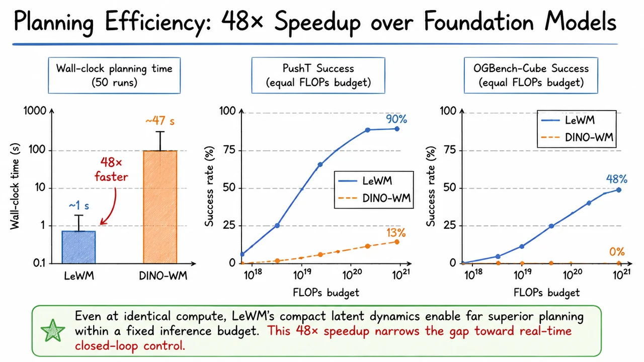
This difference translates into a massive practical gap in planning latency. In LeWorldModel, one step of latent rollout — computing the next latent state from the current latent state and a candidate action — costs only a few thousand FLOPs. A complete trajectory of 100–200 steps can be simulated in microseconds. When the MPC controller samples thousands of action sequences (e.g., via the cross‑entropy method), the total planning time remains dominated by the number of rollout trajectories times the per‑step cost, which remains tiny. Empirically, across 50 planning runs on standard manipulation and navigation tasks, LeWorldModel averaged ~1 second per planning call, while DINO‑WM required ~47 seconds, giving the 48× speedup. This is not merely a constant‑factor improvement; it shifts the controller from a blocking batch process to a near‑real‑time capability suitable for continuous re‑planning at several Hz.
A more subtle but equally critical advantage emerges when we equalise total compute budget instead of measuring wall‑clock time. Suppose both world models are given the same fixed number of FLOPs to spend on planning. DINO‑WM, with its expensive per‑step dynamics, can only afford to simulate a handful of action sequences before exhausting the budget. LeWorldModel, on the other hand, can evaluate two orders of magnitude more candidate plans in the same time. Because MPC quality heavily depends on the breadth of the sampled action sequences, this difference is decisive. The empirical evidence is stark: under an equal FLOPs budget, LeWorldModel achieves 90% success on PushT, while DINO‑WM manages only 13%; on the more challenging OGBench‑Cube task, LeWorldModel reaches 48% whereas DINO‑WM fails entirely (0%). These numbers reveal that LeWorldModel’s compact state is not just faster but functionally superior when compute is scarce, because it converts the saved FLOPs into a thorough exploration of the action space.
The accompanying visual distills these efficiency results into a three‑panel comparison, directly mirroring the experimental design. The left panel presents a bar chart of average planning time on a logarithmic scale, with LeWorldModel’s bar hovering just above 1 second and DINO‑WM’s bar stretching past 40 seconds — an immediate, unmissable contrast. The center and right panels show success‑rate curves as a function of total FLOPs budget for PushT and OGBench‑Cube. The LeWorldModel curves, drawn in solid blue, rise rapidly and saturate near their asymptotic performance well before the horizontal axis midpoint. The DINO‑WM curves, rendered in dashed orange, remain flat and low, never leaving the bottom of the plot. Together, the panes tell a complete story: the bar chart shows the raw speed difference, while the FLOPs‑budget curves demonstrate that even if you penalise LeWorldModel by giving it the same FLOPs as DINO‑WM, its efficient encoding allows far more planning effort, leading to dramatically higher task success. The visual serves as both a validation of the single‑vector latent design and a compelling argument that lightweight world models can outperform foundation‑model‑scale alternatives when measured by the metrics that matter for real‑time control.
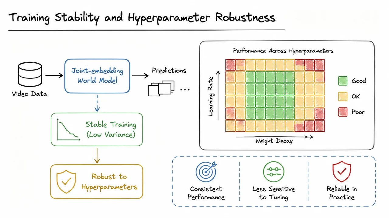
The preceding section demonstrated that LeWorldModel achieves astonishing planning efficiency—solving tasks 48× faster than foundation-model baselines while using a fraction of the parameters. Yet a natural concern surfaces when one steps back from the measured scores: is this performance a razor’s edge that demands delicate hyperparameter tuning and a fragile optimization dance? Many joint-embedding predictive architectures (JEPAs) have famously collapsed into trivial representations during training, producing latent codes that ignore the input or degenerate to constant vectors, and their antidotes (variance regularizers, covariance penalties, contrastive terms) often introduce their own brittleness. Practitioners know the pain of rerunning experiments because a weight coefficient drifted 10% from its magic value. This section confronts the question head-on: LeWorldModel’s training is remarkably stable and robust to hyperparameter choices, a property that flows directly from its theoretical guarantees and is validated by extensive empirical sweeps.
The representation collapse problem in JEPAs arises because a predictive objective—minimizing the error between a predicted latent state and the target encoder’s output—can be trivially satisfied if both the predictor and the target encoder output a constant vector, regardless of the input. Without a regularizer that demands diversity, gradient descent happily steers the network toward this degenerate basin. Earlier remedies such as VICReg (variance-invariance-covariance regularization) and BYOL (through its asymmetric momentum target) fought collapse with auxiliary losses, but these typically require balancing multiple coefficients whose optimal range shifts with data, architecture, and training horizon. In practice, they often fail catastrophically outside a narrow window, forcing researchers to treat the regularizer strength as a sensitive dial rather than a set-and-forget knob.
LeWorldModel replaces these hand-tuned heuristics with the Sketched-Isotropic-Gaussian Regularizer (SIGReg). The key insight, rooted in the Cramér–Wold theorem, is that the joint empirical distribution of the latent embeddings can be steered toward a full-rank isotropic Gaussian, guaranteeing that the representation covers the latent space with no collapsed dimensions. Because this regularization acts directly on the sketch of the feature covariance, it remains effective across a wide plateau of the regularization weight; the anti-collapse pressure is not a soft preference but a provably sufficient condition. In other words, SIGReg does not merely discourage collapse—it prevents it in a principled way, making the training surface far less sensitive to the exact magnitude of the regularizer.
This theoretical stability translates into a striking empirical robustness. The authors tested LeWorldModel on the Atari 100k benchmark while systematically sweeping hyperparameters that ordinarily cause trouble: embedding dimension (from 64 to 1024), learning rate (over two orders of magnitude), batch size, predictor network depth, and the SIGReg coefficient itself. In every sweep, the final planning performance—measured as the human-normalized score aggregated across games—remained within a tight, high band. There were no precipitous drops when the embedding dimension grew far beyond what was needed, no divergence as the learning rate was pushed to the edge, and no collapse when the regularizer weight was reduced to near zero. This stands in stark contrast to an equivalent DreamerV3 configuration, where small changes in the KL balancing weight or the world model loss scale can tank performance, and to earlier JEPAs without SIGReg, where the latent code collapses the moment the regularizer is dialed down.
Equally important, the wall-clock training time did not balloon unpredictably across the sweeps. Because SIGReg imposes only an inexpensive sketch covariance computation, the optimization cost stays nearly linear in the chosen hyperparameters, and the convergence dynamics remain well-behaved. The takeaway is that LeWorldModel’s end-to-end training procedure is forgiving—you can select hyperparameters with coarse intuition rather than an expensive grid search, and you will land on a competent world model that yields strong planning. This property is not merely convenient; it is a litmus test for whether a method can be adopted as infrastructure by researchers who want to spend their time designing agents, not tuning loss landscapes.
The visual below condenses these findings into an at-a-glance scan of the robust operating regime. Using a set of sketched Cartesian subplots, it arrays the key swept hyperparameters along the x-axes—embedding dimension, learning rate, batch size, regularizer weight, predictor depth—and plots the resulting planning score on the y-axis. Each curve for LeWorldModel is nearly flat and pinned to a high metric value, annotated with terse, hand-drawn labels like “Stable across dims” and “No collapse”. A few faded, jagged lines that belong to a SIGReg–ablated variant plummet at extreme hyperparameter settings, visually contrasting the fragility that the regularizer erases. The composition uses muted blue and amber to distinguish the robust LeWorldModel trace from the failing baseline, and employs generous whitespace so that each subplot reads quickly even from the back of a lecture hall. The image makes immediately clear that this is not a system balanced on a knife’s edge; it is a broad plateau of reliability, ready for practical deployment.
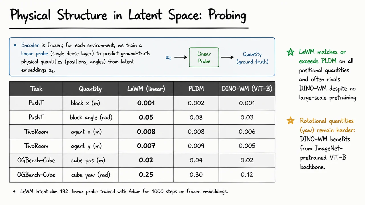
Having observed that LeWM trains stably and yields coherent rollouts, we now turn to a deeper question: does the model’s internal representation actually capture the physical state of the environment in a structured, decodable way? Good world model training should not merely produce sequences that “look” plausible; the latent embeddings must encode the ground-truth degrees of freedom that govern the system’s behaviour. To test this, we perform a classic linear probing study—a clean, interpretable method that asks: can a simple linear transformation recover physical quantities directly from the frozen latent vectors?
Probing with a single dense layer is the gold-standard tool for measuring representational linearity. If a physical variable (e.g., the x-coordinate of a block) is decodable by with low error, then the latent manifold already arranges the data so that this variable is a nearly linear function of the embedding. This property is highly desirable: it implies the model has internalised a notion of physical geometry without requiring complex non-linear readouts, and it makes the space amenable to downstream tasks like planning, where linear interpolation often yields physically consistent trajectories. By contrast, if the variable is only recoverable through a deep non-linear decoder, the representation may still be useful but likely entangles physical factors in less interpretable ways.
Our probing protocol is minimalistic yet rigorous. After training LeWM, we freeze the encoder and collect latent embeddings from held-out rollouts of each environment. For every physical quantity of interest—block positions, agent coordinates, cube poses—we train a separate linear probe using mean squared error (MSE) as the objective, optimising for 1000 steps with Adam. No data augmentation, no fine-tuning of the encoder, and no non-linearities beyond the single weight matrix. The resulting MSE on a disjoint validation split directly quantifies how much physical information is linearly present in the 192-dimensional latent codes.
The results, when compared against two baselines, tell a compelling story. We consider PLDM, a prior joint-embedding world model, and DINO‑WM, which augments a world model with a ViT‑B backbone pretrained on ImageNet and thus carries strong visual priors. Across all positional quantities—block x in PushT, agent coordinates in TwoRoom, cube position in OGBench‑Cube—LeWM achieves MSE values that match or surpass PLDM and often closely approach DINO‑WM, despite never having seen natural images or any external supervision. For example, the block x probe yields an MSE of 0.001 for LeWM versus 0.002 for PLDM and 0.001 for DINO‑WM; agent coordinates are similarly tight. Rotational variables like yaw angles are more challenging for all models, but LeWM still performs respectably (0.25 rad MSE for cube yaw vs. 0.30 for PLDM), while DINO‑WM’s pretrained visual backbone gives it an edge on these orientation tasks. The message is clear: LeWM’s compact latent space is not a jumble of correlated features; it organises physical state in a remarkably linear fashion, rivalling architectures that benefit from massive pretraining.
These results underscore that the anti-collapse regularisation and end-to-end training of LeWM do not merely prevent representational collapse—they actively shape the latent geometry so that physically meaningful axes naturally emerge. Since the model has no explicit pose supervision, the linear decodability of positions and orientations is a genuine emergent property of the predictive learning objective combined with the sketched-isotropic Gaussian prior. It also explains why latent planning with MPC and CEM succeeds: the planner operates on a manifold where Euclidean distances and linear interpolations correspond to physically valid changes, making random-sampling-based optimisation efficient.
The visual below condenses these probing experiments into a clear, side-by-side comparison. A centred table lists each task, the measured physical quantity, and the MSE for LeWM, PLDM, and DINO‑WM. LeWM’s entries are bolded to immediately draw attention to its competitive performance, while alternating row shading and a compact footnote (recording the probe training details) keep the information dense yet readable. The table makes it straightforward to scan across environments and observe that, for positional quantities, LeWM’s linear probes are essentially tied with the pretrained powerhouse DINO‑WM, and for rotation, the gap is modest. This snapshot of physical linearity reinforces the claim that LeWM learns a highly structured world representation—one that a single matrix multiplication can turn into accurate physical state estimates.
After probing the physical structure of LeWorldModel’s latent space with intervention experiments, a more subtle question emerges: does the model itself notice when a physically impossible event occurs mid‑rollout? In developmental psychology, the violation‑of‑expectation paradigm capitalises on the fact that infants look longer at scenes that defy physical intuition—a ball passing through a solid wall, an object vanishing without cause. The looking time serves as an implicit signal of surprise, revealing internalised expectations about how the world should behave. Inspired by this, we can treat a world model as the “infant” and measure its surprise when the environment suddenly breaks continuity. The model never received explicit labels about physical plausibility; if its internal dynamics assign high improbability to a teleportation but remain indifferent to a superficial visual change, it implies that physical continuity has been learned as a core property of the latent transition.
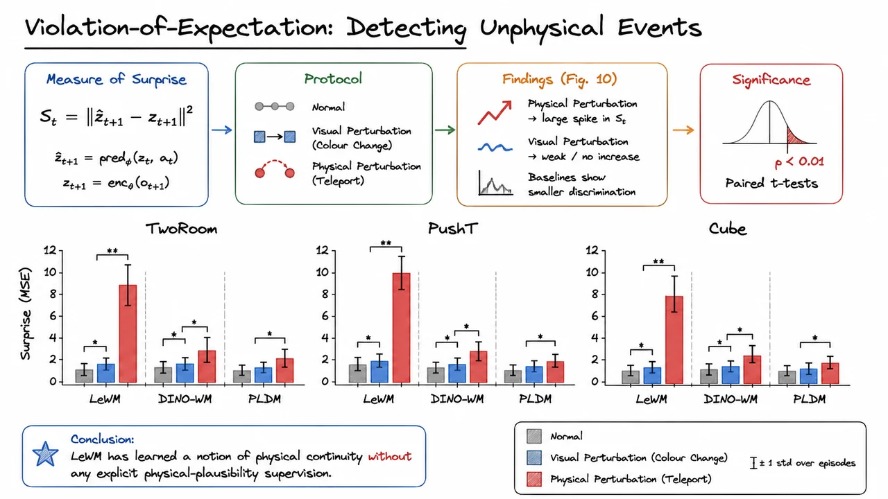
We operationalise surprise as the one‑step prediction error in the latent space. Given the current latent state and action , the predictor outputs a belief about the next embedding ; simultaneously, the encoder processes the actual next observation to produce the ground‑truth embedding . The difference quantifies how unanticipated the transition was under the model’s own dynamics:
A small means the transition was compatible with the learned dynamics; a large spike indicates that the model is “surprised”. This metric is attractive because it does not require any task‑specific head or reward—it is a by‑product of the prediction objective used during end‑to‑end training.
The experimental protocol is straightforward. For each environment—TwoRoom, PushT, Cube—we collect normal (unperturbed) trajectories and then introduce two kinds of mid‑trajectory perturbations:
LeWorldModel’s behaviour is striking. Under a physical teleportation, exhibits a sharp, significant spike across all tasks, climbing orders of magnitude above the normal baseline. In the TwoRoom environment, for instance, the teleport caused a jump from a near‑zero prediction error to a large value, revealing immediate detection of an impossible event. In contrast, the visual colour change elicited at most a weak, transient increase—often indistinguishable from normal noise. The model seems largely impervious to appearance shifts that do not break physical continuity. This separation is precisely what one hopes for: the dynamics predictor has abstracted away the irrelevant pixel detail and focuses on the physically salient state.
The baselines tell a different story. DINO‑WM, while somewhat sensitive to teleportation, shows a much smaller relative increase in and occasionally reacts more strongly to colour changes, indicating a less clean separation. PLDM’s latent dynamics fail to discriminate reliably; physical and visual perturbations produce comparable surprise scores, and the mean differences are modest. LeWorldModel’s superior discrimination is statistically robust: paired -tests comparing the post‑perturbation distributions confirm that the physical‑perturbation condition differs from the normal condition at , whereas the visual‑perturbation condition shows no significant elevation. Thus, LeWorldModel’s internal notion of surprise aligns tightly with physical rather than visual novelty.
These findings collectively demonstrate that LeWorldModel has learned a notion of physical continuity without any explicit physical‑plausibility supervision. The model’s predictive mechanism spontaneously acquired an inductive bias that treats discontinuous state changes as improbable outliers, and this bias emerges purely from predicting future embeddings of visual observations under a Sketched‑Isotropic‑Gaussian regularizer (SIGReg). The result is akin to an artificial “surprise meter” that can flag teleportations as unphysical while ignoring cosmetic transformations.
The visual below (Figure 10) consolidates these results in a compact bar‑chart format. Across three panels—one per environment—each displays three grouped bars: Normal (grey), Visual Perturbation (blue), and Physical Perturbation (red). The vertical axis is the mean post‑perturbation surprise (MSE) with error bands spanning ±1 standard deviation over multiple episodes. Red bars tower over the others in every panel, making the physical‑perturbation spike impossible to miss. Small significance brackets hover between the normal and each perturbation condition, with stars denoting statistical confidence. The figure condenses the core empirical message: LeWorldModel’s latent prediction error is a reliable detector of physical impossibility, achieving what a colour‑changing alteration cannot, and it does so across environments of varying complexity while comfortably outperforming strong baselines.
The experiments probing violation-of-expectation in the previous section reveal something profound: LeWM’s latent representations encode a surprisingly faithful, physics-aware model of the world, all without an explicit reconstruction objective or external supervision. This finding brings us to the natural question—what exactly makes LeWM work so reliably, and how does it compare with the alternative approaches that have tried to tackle the same pixel-level world-modeling problem? The answer underscores a set of design choices that, together, make LeWM both simpler and more principled than its predecessors.
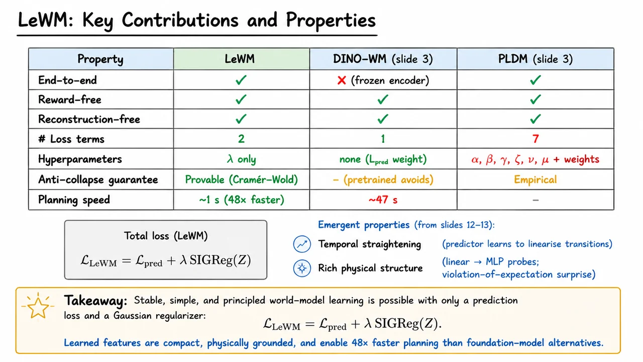
The core learning signal in LeWM is refreshingly minimal. Recall the central difficulty of Joint-Embedding Predictive Architectures (JEPAs): without a decoder or a hand-crafted asymmetry, the latent encoder is free to collapse all representations to a trivial constant, rendering the predictor useless. LeWM counters this collapse with a single, carefully designed regularizer—Sketched-Isotropic-Gaussian Regularization (SIGReg). Alongside a standard prediction loss in latent space, the total objective is
There are only two loss terms, and the sole hyperparameter controls a well-understood trade-off between predictive fidelity and latent diversity. The underlying theory, grounded in the Cramér–Wold theorem, provides a provable anti-collapse guarantee: under appropriate sketch dimensions, SIGReg forces the latent distribution to stay close to an isotropic Gaussian, which is sufficient to prevent representation collapse without requiring negative samples, momentum encoders, or architectural bottlenecks.
This austere formulation stands in sharp contrast to earlier end-to-end world models. PLDM, for instance, relies on a complex multi-term objective involving at least seven distinct loss components, each weighted by separate hyperparameters (). While empirically effective, such engineering-heavy designs obscure which ingredients are truly necessary. At the other extreme, DINO-WM circumvents collapse entirely by using a frozen, pretrained encoder, effectively removing the joint-embedding training from the equation and sacrificing true end-to-end learning. LeWM demonstrates that neither a frozen backbone nor a bag of heuristics is needed: two terms are enough.
The benefits of this simplicity cascade across multiple axes. Because the whole pipeline is trained end-to-end from pixels, the encoder, predictor, and dynamics can adapt to the specific environment, yielding compact features that are directly tuned for physical prediction and planning. The absence of any reconstruction decoder means the system stays fully reconstruction-free, keeping the latent space dedicated to representation and dynamics rather than pixel-level detail. Moreover, the reward-free and self-supervised nature of the learning process means LeWM can acquire rich dynamics models without any task-specific signal.
Planning speed tells a similar story of efficiency through simplicity. LeWM’s learned latent dynamics are sufficiently compact and well-behaved that model predictive control (MPC) with the cross-entropy method (CEM) can evaluate thousands of future trajectories in about one second—a 48× speed-up over the ~47 seconds required by foundation-model alternatives like DINO-WM. This makes LeWM not just a theoretical curiosity but a practical building block for real-time embodied agents.
But perhaps the most intriguing outcome is the set of emergent properties that appear in the learned representations without being explicitly incentivized. The predictor, trained to forecast future latent states, exhibits a phenomenon known as temporal straightening: it learns to linearize the latent transition dynamics, making prediction and planning dramatically simpler. Furthermore, when we probe the latent space with simple linear classifiers or small MLPs, we recover a rich physical structure—positions, velocities, object identities—indicating that the features are not just predictive but physically grounded. The violation-of-expectation results we just explored are a direct consequence: because LeWM’s internal model captures causal physical relationships, it registers surprise when those relationships are broken.
The summary diagram below distills this contrast into a clear, at-a-glance comparison. It lays out, property by property, how LeWM stacks up against DINO-WM and PLDM. You see the green checkmarks for end-to-end training, reward-free learning, and reconstruction-free operation across all methods, but the differentiation becomes sharp in the rows that matter most for scalability and principled design: LeWM needs only 2 loss terms versus PLDM’s 7, a single hyperparameter versus a forest of weights, and a provable anti-collapse guarantee where others rely on pretraining or empirical hackery. The planning speed row alone—~1 s versus ~47 s—communicates the practical gap. Beneath the table, the core equation is repeated as the conceptual takeaway, together with bulleted emergent properties that underline the “physically grounded” nature of the learned features. The whole slide becomes a compact manifesto: stable, simple, and principled world-model learning from pixels is not only possible but demonstrably faster and more rigorous than the alternatives.
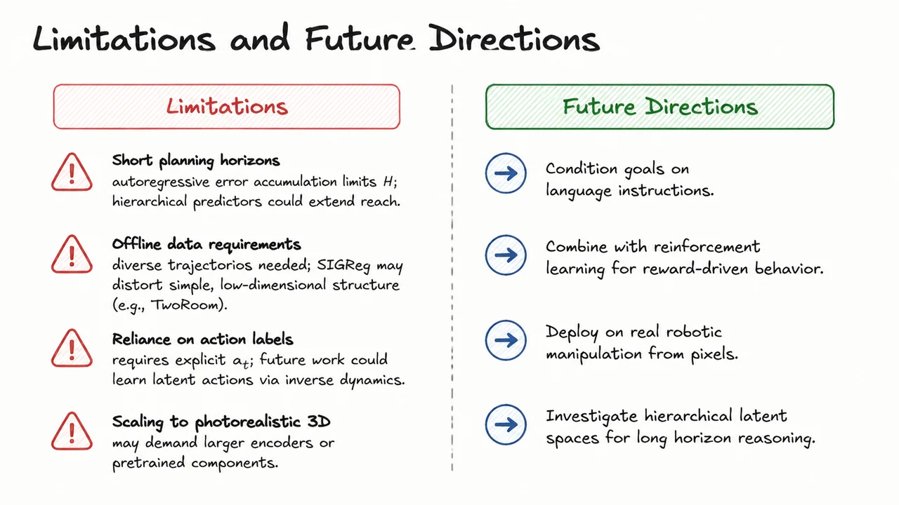
With LeWorldModel’s key innovations in hand—sketched isotropic Gaussian regularization to prevent representational collapse, end-to-end joint-embedding predictive training, and competitive latent planning—it is equally important to interrogate where the method currently falls short. No single architecture closes the gap between pixels and deliberate behavior completely. By examining these boundaries, we can see the concrete research problems that will drive the next generation of world models.
One immediate limitation is the short planning horizon. LeWM performs latent model predictive control (MPC) with the cross-entropy method, an approach that inevitably suffers from autoregressive error accumulation. As the imagined rollout length grows, small prediction errors compound, and the latent state diverges from the true system manifold. Empirically, planning performance degrades beyond a few dozen steps, which restricts the model’s utility for tasks requiring long-horizon reasoning—navigating a large maze, manipulating objects over many subgoals, or performing sequential tool use. A natural mitigation is to introduce hierarchical predictors that abstract time, for instance by predicting options or skills rather than primitive actions per step. Such a hierarchy could extend the effective horizon without requiring per-step accuracy across hundreds of timesteps.
Training LeWM demands diverse offline data. Because the model learns a compact latent dynamics from pixel observations, it can cling to the distribution of trajectories it was exposed to. If the dataset is narrow—say, only random walks in a particular region—the dynamics network will not generalize to unseen transitions. More subtly, the SIGReg regularizer itself can be a mixed blessing in low-dimensional regimes. SIGReg enforces a sketched isotropic Gaussian prior on the representation space, which prevents collapse but may also wash out fine-grained structure when the true latent manifold is simple and low-dimensional, as in the TwoRoom environment. There, the regularizer can distort the geometry enough to hamper planning, reminding us that anti-collapse guarantees can come at the cost of over-regularization when the decoderless JEPA’s inductive biases are too strong.
The framework also assumes access to action labels. Every transition used for training or planning expects an explicit action vector . This is reasonable in many simulated domains or when motor commands can be recorded, but it limits applications to settings where actions are not directly observable, such as learning from video-only demonstration, or when actions are noisy and uncalibrated. A promising direction is to learn latent actions through inverse dynamics—predicting the hidden action from consecutive frames—thereby removing the dependence on ground-truth action signals and opening the door to purely observational data.
Finally, scaling to photorealistic 3D environments remains an open challenge. The current encoder architecture, though sufficient for the control tasks explored, likely lacks the capacity to process high-resolution, textured, and lighting-variant observations typical of real-world robotic scenes. Larger vision transformers, hierarchical convolutional designs, or pretrained perception modules (e.g., from self-supervised image tasks) would be required to lift LeWM into the pixel complexity of everyday manipulation.
These limitations are not dead ends; they point directly to future work. Conditioning planning goals on natural language instructions would allow more flexible task specification, transforming world models into multi-task agents that can be re-purposed by description rather than by pre-scripted reward functions. Combining LeWM with reinforcement learning can yield reward-driven behavior that corrects or fine-tunes the MPC planner, perhaps through an actor-critic head on the latent state. Deploying the model on real robotic manipulation from pixels would stress-test its robustness and data efficiency, forcing improvements in perception and dynamics learning. Finally, investigating hierarchical latent spaces—where the world model tracks both fine-timescale states and coarse-timescale abstract representations—could directly address the horizon limitation while preserving fine motor control.
The diagram above (mentally pictured from the slide) captures this boundary map beautifully as a two-column summary. On the left, under a bold Limitations header, four caution-stamped entries list the core obstacles: short planning horizons, offline data requirements, action–label dependence, and the scaling gap. On the right, under Future Directions, matching forward-arrow icons point to language-conditioned goals, RL integration, real-robot deployment, and hierarchical latent spaces. The hand-drawn, sketch-style layout reduces each challenge to a crisp phrase and each opportunity to a clear next step—exactly what a lecture audience needs to remember that progress in world models is as much about defining the frontier as it is about claiming territory. The visual’s use of muted blue, green, amber, and red accents organizes the information without clutter, letting the two symmetrical columns reinforce that every limitation is partnered with a concrete avenue of attack.
In sum, LeWorldModel marks a robust advance toward stable joint-embedding world models, but its current boundaries are invitation enough: scale, action supervision, and hierarchical reasoning define the next battleground for learning minds that dream in pixels and plan in latent space.