The modern story of the Transformer begins not with attention itself, but with a computational constraint that had quietly shaped most neural sequence models. Before self-attention became the centerpiece of an architecture, sequence transduction—mapping one sequence to another, as in machine translation, speech recognition, or text summarization—was dominated by recurrent encoder-decoder models. These models processed an input sequence step by step, maintaining a hidden state that was supposed to carry forward a compressed summary of everything seen so far. That approach worked well enough on moderate-length sequences, but it carried a structural cost that became increasingly hard to ignore.
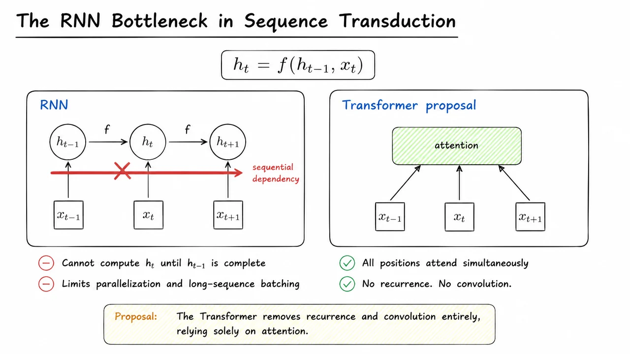
At the center of that cost is a deceptively simple equation. In a recurrent network, the hidden state at position is typically written as
where is the representation of the input symbol at position , is the previous hidden state, and is some parameterized transition function—an Elman RNN cell, an LSTM, or a GRU. The notation looks innocent, but it encodes a strict temporal chain: before the model can compute , it must already have computed . There is no way around that dependency within a single recurrent layer. Information about can influence only by being carried forward through , one transition at a time.
This factorization imposes sequential computation along the time axis. It is not merely an implementation detail; it follows directly from the mathematical form of recurrence. Because every hidden state depends on the previous one, the operations cannot be fully parallelized within a training example. A GPU can process many independent examples in a batch at once, but time steps inside each sequence must still be unrolled in order. For long sequences, the number of serial operations grows linearly with sequence length. In practice, that means longer training times, worse hardware utilization, and additional difficulty when batching sequences of very different lengths.
The consequences are both computational and architectural. The serial bottleneck matters for at least three reasons. First, it limits parallelism: each time step waits for the previous one, leaving many processing units idle at the temporal level. Second, long-range dependencies become harder to learn, because a signal from an early token must survive many nonlinear updates in a fixed-size hidden state before it can affect a later prediction. Third, the hidden state becomes a summary bottleneck: it must compress all prior context into one vector of fixed capacity, even when the model would benefit from directly inspecting an earlier token. These are not absolute failures—LSTMs and GRUs were explicitly designed to mitigate vanishing gradients and improve memory—but the fundamental sequential dependency remains.
Attention offered a promising alternative, but for some time it was used only as a supplement to recurrence. Classic encoder-decoder attention allowed the decoder to look directly at encoder states when generating each output token, rather than relying solely on the encoder’s final hidden state. That already improved long-range behavior in many tasks. However, the encoder and decoder themselves were still recurrent. Attention could reach across positions, but the computation still moved through time in the usual unrolled recurrent fashion. In that sense, attention had not yet eliminated the bottleneck; it had only softened one of its symptoms.
The core proposal behind the Transformer is to remove recurrence altogether—and with it, the hidden-state recursion in . Instead of passing information along a sequential chain, the Transformer lets each position interact directly with the others through attention. In the simplest motivating view, every input position can be connected to every other position in a single computation step, so the model no longer needs to wait for the previous hidden state. Convolution was also removed, because although convolutional layers parallelize well across positions, they do not naturally connect distant positions without stacking many layers or using large receptive fields. The result is an architecture built from attention, point-wise nonlinearities, and carefully designed positional signals.
The visual below condenses this contrast into two panels. On the left, an unrolled recurrent chain shows hidden states connected by forward arrows, with inputs entering from below and a thick red crossed-out arrow marking the sequential dependency. That crossed arrow is the real obstacle: it says that information cannot jump from one position to another without passing through all intermediate states. On the right, the proposed architecture replaces the recurrent chain with an attention block that receives inputs from and simultaneously. There is no recurrent arrow connecting positions; instead, direct edges suggest that each position can exchange information with the others in parallel.
This visual is not meant to make recurrence look inherently wrong—many biologically inspired and time-series models remain recurrent for good reason. Rather, it isolates the specific constraint the Transformer is designed to remove. Once the recurrent arrow disappears, the architecture is free to compute all positions at once, to compare all pairs directly, and to scale much more efficiently across modern parallel hardware. That single structural change is the foundation on which the rest of the Transformer is built.
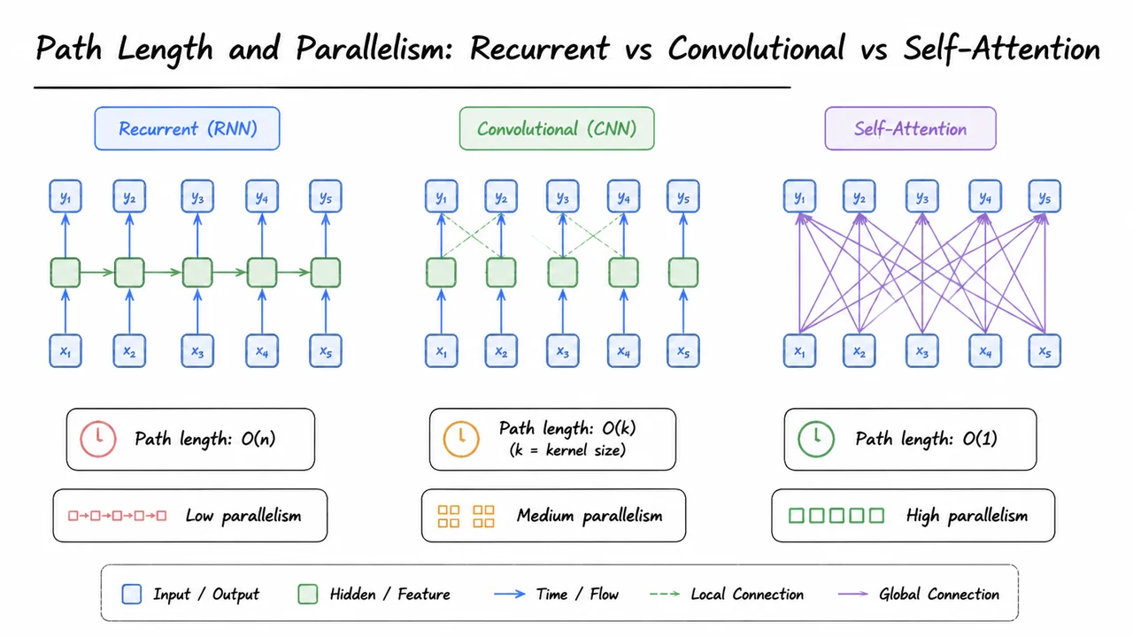
The previous section measured the cost of moving information across a sequence: a recurrent network must pass a hidden state through sequential steps, a convolutional stack expands its receptive field gradually with depth, and self-attention gives every pair of positions a direct path in a single layer. That result is a property of an attention primitive, not yet a complete learning system. The Transformer turns this primitive into a full sequence-to-sequence model by arranging attention, pointwise nonlinear transformations, and residual connections into a deep, repeated structure: the stacked encoder-decoder architecture.
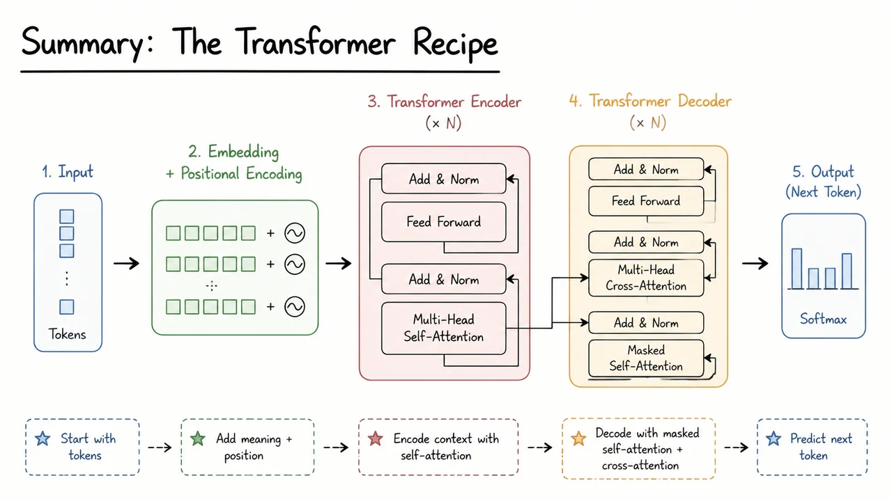
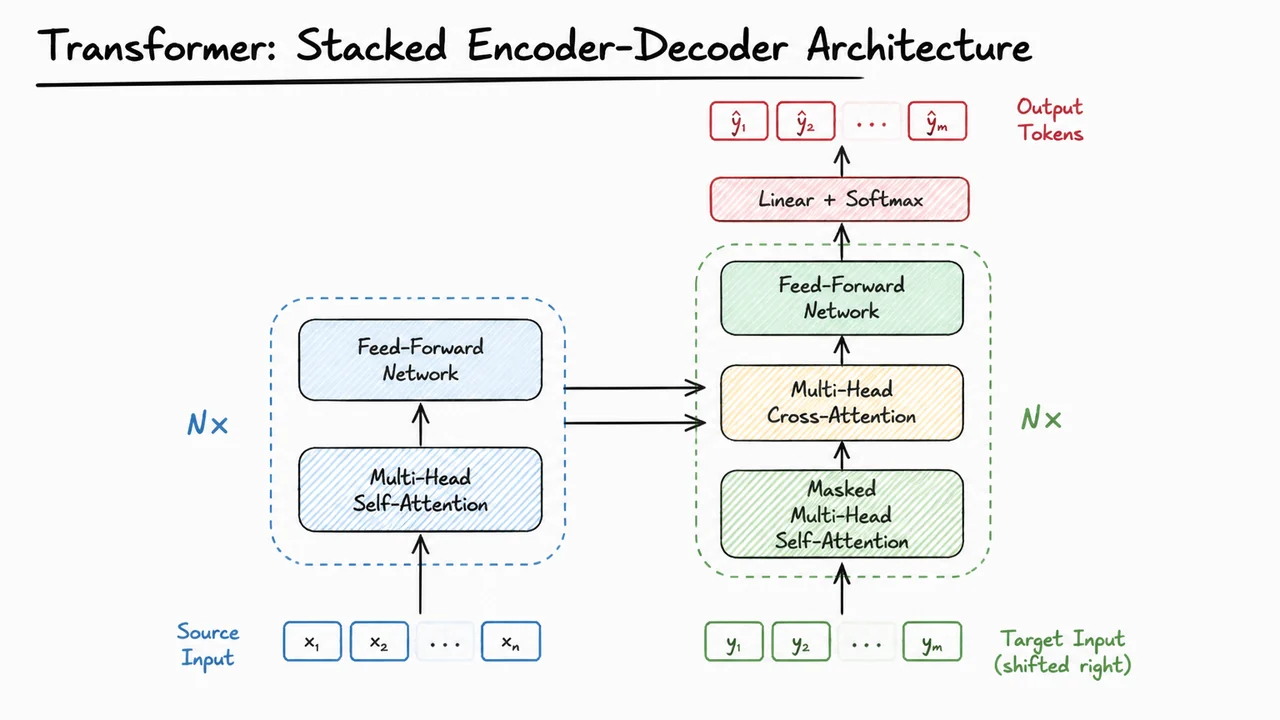
At the highest level, the Transformer keeps the familiar encoder-decoder shape of sequence transduction. The encoder reads the entire source sequence and produces a sequence of continuous representations . The decoder then generates the target sequence one token at a time, conditioned on the encoder representations and on the previously generated target tokens. What is new is the inside of the encoder and decoder. Instead of recurrent cells or convolutional layers, each side is built from a stack of identical layers whose main mixing mechanism is attention.
Each encoder layer has two sublayers. The first is a multi-head self-attention sublayer, which allows every position in the input to gather information from every other position. The second is a position-wise feed-forward network, which applies the same two-layer nonlinear transformation independently to every position. Each decoder layer has three sublayers: a masked multi-head self-attention over the target sequence, a multi-head cross-attention from the target to the encoder output, and a final position-wise feed-forward network. The masking is essential in the decoder: when predicting position , the model may attend only to positions , so the factorization remains autoregressive and future target tokens cannot leak into the past.
Around every sublayer there is a residual connection followed by layer normalization. If denotes one of the attention or feed-forward blocks, the connection can be written as
The residual connection means that the sublayer only has to learn a change to its input, and the identity path gives gradients a direct route through the stack. This is why all sublayers and embedding layers are chosen to share the same width ; otherwise the residual addition would require a linear projection. In the original Transformer , the feed-forward hidden width is , and the model uses identical layers on both the encoder and decoder sides.
A useful way to read the encoder is as repeated global refinement. In one self-attention sublayer, every token can already access every other token, so receptive field is not being built up step by step as in a convolutional or recurrent model. Stacking encoder layers therefore does not exist mainly to enlarge the receptive field. Instead, depth gives the model room to compute increasingly abstract representations of the same global context. This distinction matters for long sequences: the shortest path between two source positions remains constant with respect to sequence length, even though the model becomes deeper.
The decoder is more subtle because autoregressive generation still proceeds one output token at a time at inference. The advantage of the Transformer is not that it removes the sequential output dependency, but that it removes the sequential bottleneck in how the model computes context for each prediction. All already generated positions can be processed in parallel during training, and when predicting the next token, each known token can attend directly to earlier positions. The cross-attention sublayer goes further: every decoder position can attend directly to every encoder
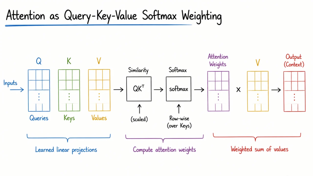
Once the Transformer is accepted as a stack of repeated encoder and decoder layers, the next question is almost inevitable: what is the actual operation inside each layer that lets one position influence another? The answer in the Transformer is not convolution or recurrence, but a form of soft, content-based retrieval called attention. Conceptually, every attention operation can be described as a differentiable dictionary lookup. Each position issues a query expressing what it is looking for, while every possible source position exposes a key describing what it offers and a value containing the information to be transferred if selected. The output for a query is then a weighted mixture of the values, where the weights come from comparing the query against all keys.
This query-key-value language is more than an analogy. Suppose we have a query vector for output position , a set of key vectors , and corresponding value vectors . A natural compatibility score is the dot product . Larger scores mean the query and key point in similar directions, so that particular value should contribute more. Because raw scores can have arbitrary scale and need to be interpreted as relative preferences, they are passed through a softmax over all keys for each query:
The resulting weights are nonnegative and sum to one, which makes the output a convex combination of values:
In matrix form, with query matrix , key matrix , and value matrix , this becomes
where the softmax is applied independently to each row of the scaled score matrix. The scaling factor keeps the dot products from growing with the key dimension; the precise rationale is important enough to deserve its own treatment, but for now it is enough to notice that it prevents the softmax from becoming pathologically saturated.
There are several subtle assumptions in this formulation. First, queries and keys must live in the same vector space for the dot product to be meaningful, whereas values may have a different dimension. Second, the softmax creates a competition among keys for each query: if the scores are similar, attention spreads across many values; if one score dominates, the output becomes very close to that single value. Third, the number of outputs is determined by the number of queries, not by the number of keys and values. This is why a decoder can produce a shorter or longer output sequence while attending over the entire encoder representation. In self-attention, queries, keys, and values all come from the same sequence, but in cross-attention they come from different sequences.
This operation has several architectural consequences. It is permutation equivariant in the absence of positional information, meaning that if the input positions are shuffled, the attention outputs are shuffled in exactly the same way. That is one reason the Transformer needs explicit positional encodings. It also gives each pair of input and output positions a direct computational path of length one, unlike recurrent models where information must pass through intermediate hidden states. On the other hand, the cost is quadratic in the sequence length because every query is compared with every key. This is the main trade-off that later efficient-attention variants attempt to improve.
A useful way to internalize the operation is to split it into three mental stages. First, compute query-key compatibility scores. Second, turn those scores into a probability distribution with softmax. Third, use that distribution to take a weighted average of values. This keeps the operation smooth and end-to-end differentiable while still allowing the model to focus sharply on the most relevant positions when needed.
The visual below condenses this pipeline into a single schematic. A query vector is compared with several key vectors, producing raw match scores represented by simple bars. The softmax step rescales those bars into normalized weights, often shown with size or color intensity, and those weights are then applied to the corresponding value vectors. The final vector is drawn as the sum of the weighted value contributions, making it visually clear that attention is not selecting a single value but blending all values according to learned relevance.
Understanding this soft weighting primitive is the foundation for the rest of the Transformer. It explains why the architecture can route information dynamically based on content rather than being limited to a fixed local neighborhood or a sequential hidden state. From here, the natural next step is to inspect the scaled dot-product operation more closely: why the scaling constant is exactly , how the row-wise softmax behaves in high dimensions, and how the whole computation is expressed as a compact set of matrix operations.
After seeing attention as a softmax weighting over values, the natural next question is how to compute the compatibility between a query and each key. The Transformer answers this with a particularly simple choice: a dot product. For a single query and a key , the unnormalized score is
When all queries and keys are packed into matrices, the entire score matrix can be obtained with one matrix multiplication,
where , , and . Each row of contains the compatibility scores from one query to all keys. Softmax is then applied per row, and the resulting attention weights multiply . This gives the compact form
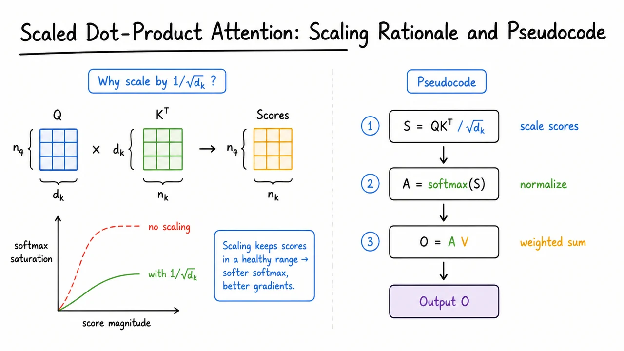
The division by is the part that deserves real attention, because it is not just a cosmetic normalization.
The scale factor addresses a statistical problem with high-dimensional dot products. Suppose the components of and are independent random variables with zero mean and unit variance. Then each product term has mean zero and unit variance as well, and the sum over dimensions has variance . In other words,
The typical magnitude of a dot-product score therefore grows like . For large , raw scores can become strongly positive or strongly negative. Once those logits enter a softmax, they saturate: the resulting attention distribution becomes nearly one-hot, and the gradient of the softmax with respect to the logits becomes extremely small. Training slows down, and the attention mechanism loses the useful interpolative behavior that softmax weighting is meant to provide.
Dividing by is thus a variance-stabilizing transformation. It keeps the scale of the logits roughly independent of the model width, at least under the random-initialization or zero-mean assumptions. From a probabilistic perspective, this is also a temperature adjustment. Writing the softmax as
shows that the raw dot-product attention uses , while scaled dot-product attention uses . A larger temperature makes the softmax distribution softer, counteracting the tendency of large- dot products to over-sharpen. This is why the mechanism is called scaled dot-product attention.
There is also a practical and historical comparison here. Additive attention, popular in earlier sequence-to-sequence models, computed compatibility through a small feed-forward network, often
That form does not inherently need the same correction, but it is slower to compute. Dot-product attention is attractive because it reduces scoring to highly optimized matrix multiplications. The original Transformer paper notes that additive attention can outperform unscaled dot-product attention for larger key dimensions, but with the scaling, dot-product attention becomes both fast and stable.
The full computational recipe is therefore short. Conceptually, the operations are:
A minimal pseudocode form is:
scores = Q @ K.transpose(-2, -1) / sqrt(d_k)
if mask is not None:
    scores = scores.masked_fill(mask, -inf)
weights = softmax(scores, dim=-1)
output = weights @ V
The optional mask matters in transformer decoding. In autoregressive generation, a query at position must not attend to future keys . Adding a causal mask before softmax sets those scores to , so their probabilities become zero. Padding masks play a similar role for ignored input positions in batched sequences.
The visual summary below condenses this entire idea into a small functional diagram. It shows the stream from , , and through the matrix multiplication , then through the scale block, the optional mask, the softmax, and finally the second matrix multiplication with . The placement of the scaling block right after the first matmul is the crucial detail: it visually marks the point where high-dimensional dot products are brought back to a range where softmax can produce informative, gradient-friendly attention weights rather than saturated one-hot outputs.
Once scaled dot-product attention is a well-defined primitive, the next architectural question is whether one such attention operation is enough. A single attention head produces a weighted average of values, where the weights reflect one particular compatibility score between queries and keys. That can already capture many relationships, but it imposes a strong constraint: every position must use the same notion of relevance at a given layer. In natural language, relevance is rarely one-dimensional. A word may need to attend to a syntactically related verb for agreement, to a nearby modifier for adjective-noun structure, and to a coreferent entity many tokens away, all at the same time. If a single attention mechanism tries to encode all of these relationships, their signals can interfere and compete for the same softmax probability mass.
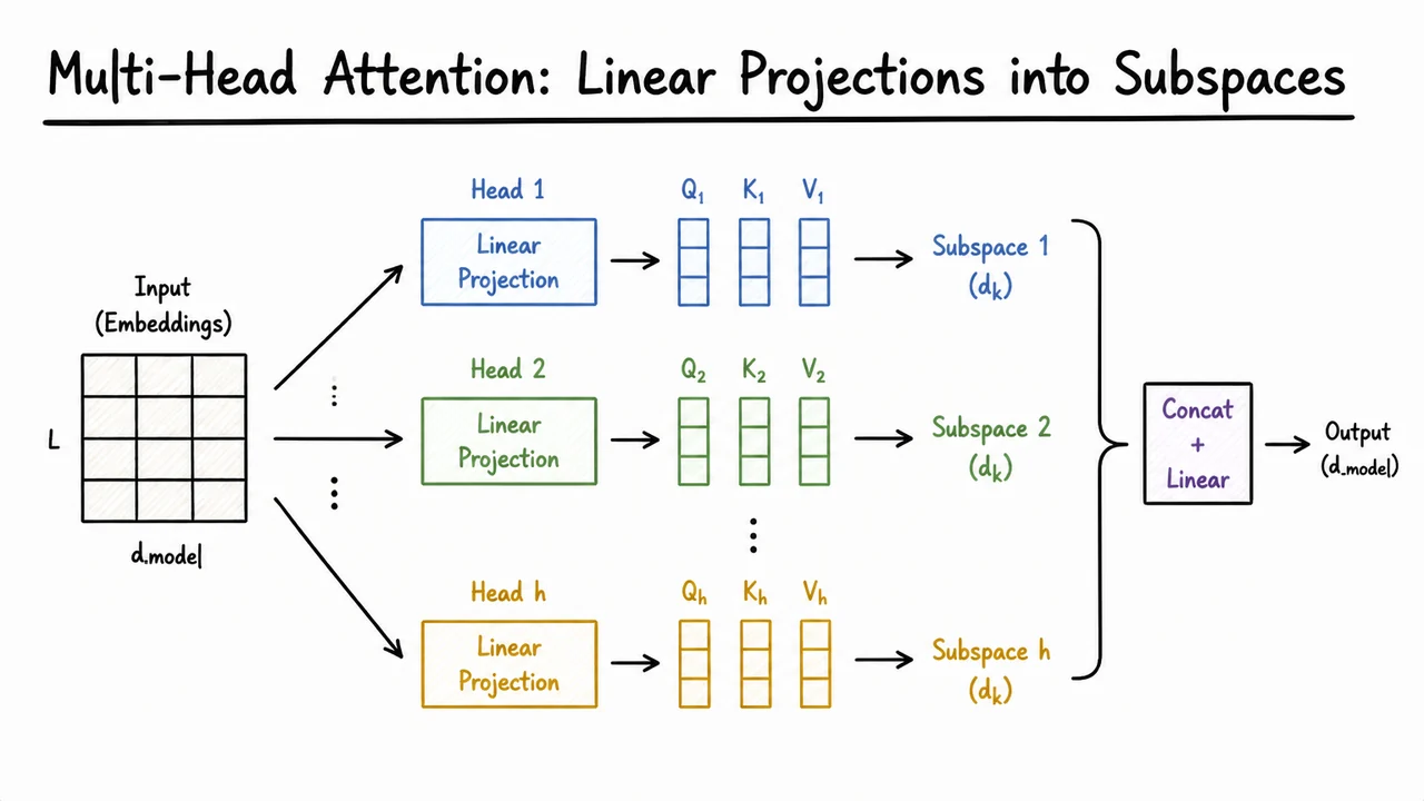
Multi-head attention addresses this by running several attention operations in parallel, each operating on a different learned representation of the queries, keys, and values. Instead of one large attention function over the full -dimensional hidden state, the Transformer projects the same queries, keys, and values times into lower-dimensional subspaces. For the -th head, learned projection matrices
transform the original matrices into head-specific inputs:
Each head then computes scaled dot-product attention on these projected versions:
The projections are not a fixed decomposition into existing axes. They are learned linear maps, so each head can learn to form new axes that are useful for a particular kind of relevance. A query projection might emphasize syntactic features, while another head’s query-key pair might learn to emphasize semantic similarity or positionally local content.
The fact that the projections go from a larger space into a smaller one is deliberate. In the original Transformer, , , and , so each head operates in a 64-dimensional subspace rather than the full 512-dimensional representation. This keeps the total computational cost close to that of a single full-dimensional attention head, because eight dot products of width 64 have roughly the same cost as one dot product of width 512. Yet the eight heads have independent parameter matrices, so they can learn eight different compatibility criteria rather than forcing a single criterion to do all the work.
A useful way to think about each head is that it defines a learned compatibility metric. The pre-softmax score between a query and a key in head is
Since both sides are projected into , the learned matrix can represent only a family of bilinear forms whose rank is bounded by . This is a form of regularization: the head cannot use arbitrary high-dimensional interactions between query and key directions. It must compress the interaction into a small subspace, which encourages the model to discover the most predictive low-dimensional structure for each head.
The parallel structure also introduces a useful inductive bias. If the model has eight separate heads, there is no explicit rule forcing them to specialize. Nothing in the loss function says “head one must track long-range dependencies” or “head two must handle local syntax.” Instead, specialization arises because each head has lower capacity than the full model and because backpropagation tends to assign different functions to different parameter groups when they must collectively reconstruct useful outputs. Empirically, many trained Transformer models do show distinct attention patterns across heads, with some heads attending locally, others attending broadly, and some attending to specific syntactic relations. This diversity is not guaranteed in every model, but the architecture makes it possible.
There is also a practical reason for projecting queries and keys into separate subspaces. If queries and keys used the same projection, compatibility would be governed by a symmetric measure such as inner product in a shared space. Separate and matrices allow asymmetric relationships: what makes something a good query may differ from what makes something a good key. For example, in retrieval terms, the query “what is the capital of France” and the key “Paris is located in northern France” do not need to be represented identically; they only need to produce a high compatibility score after their respective projections.
The visual below condenses this projection stage. It treats the original query, key, and value tensors as a single common input block, then draws parallel arrows through distinct projection triples. Each arrow narrows into a smaller query, key, and value subspace, visually marking the dimensional reduction from to or . That narrowing is the core idea of this part of the Transformer: not yet the concatenation or output projection, but the moment where one representation is deliberately split into several learned views, each of which will perform its own attention computation independently.
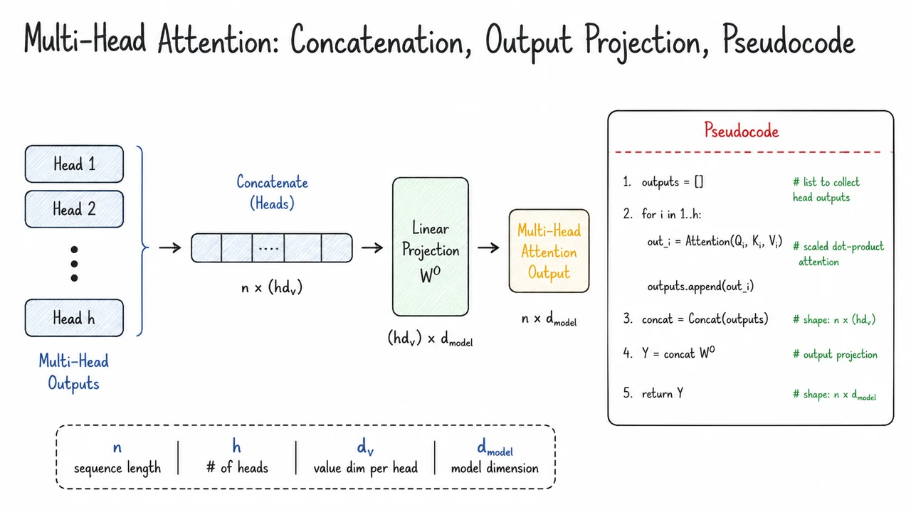
Having projected the queries, keys, and values into separate lower-dimensional subspaces, each attention head has now produced its own independent output. Those outputs are not yet a single representation: they live in different projected feature spaces, and the rest of the Transformer expects one vector of width . The next step is therefore about reassembly. The Transformer uses a two-stage operation: concatenate all head outputs, then apply a final learned linear projection back to the model dimension.
Formally, let each head compute
where , , and . Each head output is therefore a -dimensional vector per token. Concatenating across all heads gives a vector of size . Multi-head attention then applies one more learned matrix:
where . This output projection restores the representation to the model width, allowing it to pass cleanly into the residual stream and subsequent sublayers.
It is tempting to view merely as a dimension-changing convenience, but it is a learned mixing layer. If we partition into blocks , the concatenation-plus-projection can be rewritten as a sum of per-head contributions:
[ \text{Concat}(\text{head
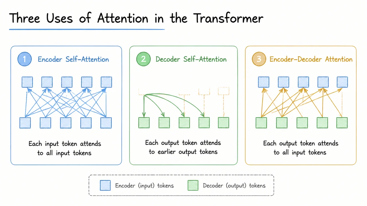
Having worked through the mechanics of multi-head attention, we are now in a position to ask the architectural question: where exactly should this operation sit in a sequence-to-sequence model? The Transformer’s answer is surprisingly uniform. It does not introduce three completely different kinds of sequence mixing; instead, it uses one attention primitive—scaled dot-product multi-head attention—in three distinct roles, distinguished mainly by where the queries, keys, and values come from. That data-flow distinction is enough to create bidirectional encoding, causal decoding, and source-conditioned generation.
Before looking at the three concrete roles, it helps to separate self-attention from cross-attention. In self-attention, the queries, keys, and values are all produced from the same sequence representation. This lets each element compare itself to every other element in the same sequence. In cross-attention, the queries come from one sequence while the keys and values come from another sequence. The attention operation remains mathematically unchanged:
but the semantic meaning changes dramatically because the compatibility scores now measure relevance between two different spaces.
The first use is encoder self-attention. In every encoder layer, the queries, keys, and values are computed from the previous encoder layer’s output. For the very first layer, that input is the sum of token embeddings and sinusoidal positional encodings. Because the encoder processes the full source sentence at once, this attention is unmasked: each position may attend to every other position, including itself. The result is a contextualized representation of every token that can draw directly on long-range syntactic or semantic dependencies without recurrence. If a verb at the end of a sentence needs information from its subject near the beginning, that dependence is one attention step away.
The second use is decoder self-attention, which is deliberately restricted. The decoder is autoregressive: it predicts the next target token from previously generated tokens. During training, the model may have access to the whole target sentence, so without care the decoder could cheat by peeking at future tokens. The Transformer prevents this with a masked self-attention mechanism. Before the softmax is applied, all scores corresponding to positions after the current one are set to , so their attention weights become zero. This preserves the causal property:
at training time and matches the inference-time constraint that future tokens are not yet known. The mask is usually implemented as an upper-triangular additive mask over the matrix.
The third use is encoder-decoder attention, sometimes called cross-attention or source attention. Here the queries come from the preceding decoder layer’s output, while the keys and values come from the final output of the encoder stack. Conceptually, the encoder produces a memory of the source sentence, and each decoder position issues a query against that memory to decide which source positions are most relevant for producing the next target token. This is the only path by which source information enters the decoder. The result is a soft alignment between target and source positions, learned end-to-end rather than prescribed by a separate alignment model.
One subtle but important point is that these are not shared parameters. Each occurrence is its own multi-head attention sub-layer with its own learned query, key, value, and output projection matrices. What is shared is the form of the operation and the idea that compatibility between a query and a key should determine how much value information is aggregated. This makes the architecture conceptually compact, even though the total number of parameters grows with depth.
The payoff is visible when the three roles are placed side by side. Encoder self-attention gives every source token a full-sentence context. Masked decoder self-attention gives every target token a left-to-right causal context. Encoder-decoder attention gives every target token a window into the entire source sentence. All three preserve the constant path-length property of attention: the number of sequential operations needed for information to travel between any two positions is , subject only to masks that restrict which positions are allowed to communicate.
The visual below compresses this into three parallel panels. It makes the data flow explicit: tokens within one sequence are wired by self-attention, while the connection between source and target is carried by cross-attention. The masked future positions appear as excluded edges or shaded matrix entries, which is a concise reminder that the decoder’s causal constraint is an architectural priority, not an afterthought. Seeing the three panels together reinforces that the Transformer’s power comes from reusing a simple, parallelizable attention mechanism with carefully chosen routing of queries, keys, and values.
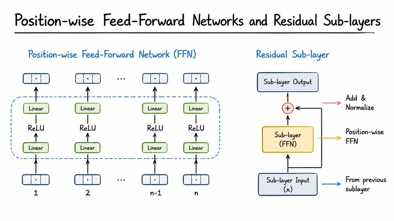
After attention has gathered information across positions, the Transformer still needs a component that can transform each token's representation independently. This is where the position-wise feed-forward network enters. The self-attention sub-layer is about mixing: every position queries the sequence and produces a weighted average of value vectors. But mixing alone does not give the model much power to compute new features. A linear combination of value vectors remains a linear operation, and stacking multiple attention layers would still amount to sophisticated linear mixing. The feed-forward sub-layer exists to inject nonlinear computation into every token representation.
The term position-wise is deceptively simple, but it carries real architectural weight. It means the same feed-forward transformation is applied to every position independently, with parameters shared across positions but not across layers. If the model dimension is , then for each input vector at one position, the network computes
where maps into a larger inner dimension , often chosen as 2048 when , and projects back down to . The is the ReLU activation. Conceptually, this is a two-layer MLP squeezed between linear projections, repeated once per token position.
Why expand the inner dimension to four times the model width? The intuition is reminiscent of the expanded middle layer in a bottleneck MLP or the temporary feature maps of a convolutional network: a wider intermediate representation gives the nonlinearity more room to form useful feature detectors, while the final projection compresses the result back to the main residual stream width. The position-wise nature also reveals an interesting connection to convolutions. If you arrange the sequence as a one-dimensional feature map of shape , a linear projection applied identically at every position is equivalent to a convolution. So the feed-forward sub-layer can be read as two convolutions with a ReLU in between, a view the original paper explicitly notes. This analogy matters because it shows the Transformer is not purely attention; it blends attention's global context with the local, per-position feature transformation familiar from convolutional design.
Just as important as the feed-forward block itself is how sub-layers are wired together. The Transformer does not simply chain outputs sequentially. Every sub-layer—whether it is multi-head attention or the position-wise FFN—is wrapped in a residual connection followed by layer normalization. If is the input to a sub-layer , the output is
The residual connection preserves a direct gradient path around the sub-layer, allowing the model to learn what the sub-layer should add rather than forcing it to reconstruct the entire representation from scratch. This is the same idea that made very deep convolutional networks trainable, and it is even more critical in the Transformer because both encoder and decoder stacks can be stacked six or more layers deep. Without residuals, the signal would degrade through repeated nonlinear blocks; with them, each sub-layer becomes a small refinement step over a stable base representation.
Layer normalization, rather than batch normalization, is the chosen stabilizer. Batch normalization would depend on problematic cross-position statistics for variable-length sequences and would complicate autoregressive decoding, where future positions are masked. Layer norm instead computes mean and variance across the feature dimension of a single token, which is independent of sequence length and batch composition. Additionally, the Transformer applies dropout to the output of each sub-layer before the residual addition, and also to attention weights and embedding outputs, acting as a regularizer that forces the network not to rely on any single sub-layer or attention head too heavily. The overall block structure is therefore: input to sub-layer, nonlinear computation, dropout, residual sum, layernorm, and pass onward.
Two subtle decisions are worth noting. First, residual connections are formulated as , so the sub-layer output must have the same dimensionality as its input. This is why attention and FFN sub-layers both end with an output projection back to . Second, the FFN is separate between layers; even though positions share parameters within one layer, the next layer learns a fresh . This gives the stack a repeated rhythm: attention mixes information across positions, then the FFN re-expresses each position's feature vector. Repeating this six times allows the representation to alternate between contextual pooling and local nonlinear feature computation, a pattern that empirically works strikingly well.
The visual below condenses this block-level design into a compact anatomy. It shows a single Transformer layer fragment as a pipeline: the input flows into the sub-layer, the sub-layer's output is added back to the input through a residual edge, and the combined result passes through layer normalization. A separate inset highlights the FFN itself as three linear stages—an expansion projection, a nonlinear ReLU, and a contraction projection—applied independently at each sequence position. The emphasis on one block, reused identically across positions is the key visual message: the Transformer is built from repeated local transformations stitched together by global attention and stabilized by residuals. Seeing the FFN and the residual wrapper side by side helps fix the two distinct levels of the design in mind: the microscopic per-position MLP, and the macroscopic skip-and-normalize topology that makes deep stacks trainable.
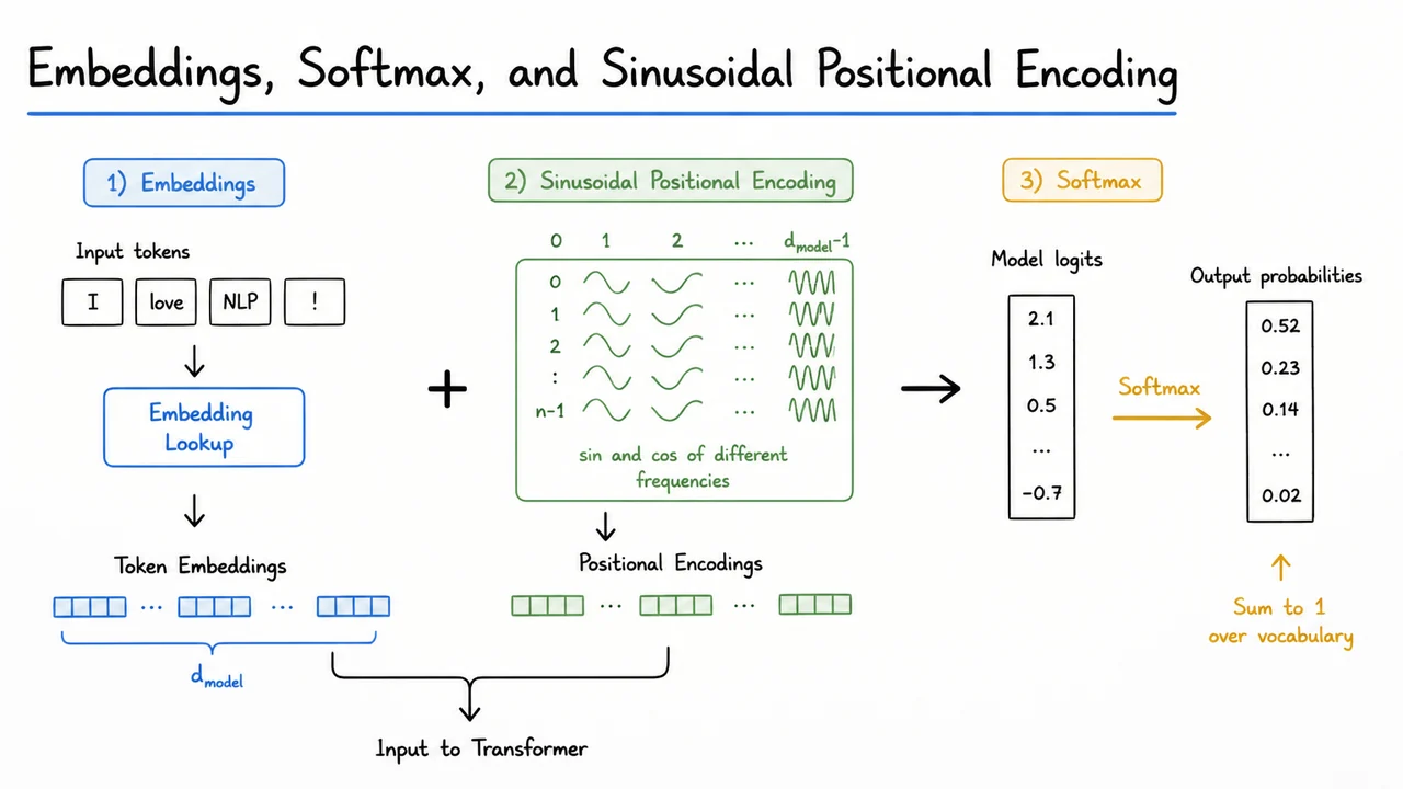
After the position-wise feed-forward sub-layer and its residual connection, every token inside the Transformer is already a rich contextual vector. But the path that turns a raw token index into that vector, and the path that turns the final decoder vector back into a token prediction, matter just as much as the attention mechanism itself. This is where the Transformer’s reuse of representations becomes especially clean: one learned embedding table, one softmax, and a deterministic sinusoidal signal for word order.
Both the encoder input tokens and the decoder output tokens are first converted into vectors of dimension . If the vocabulary has tokens, the model stores an embedding matrix . A token index selects a row , which may be interpreted as a learned, dense representation of that token before any context is observed. The original Transformer scales this embedded vector:
The scaling is subtle. It is not required for the token representation itself, but it becomes important when the token embedding is added to the positional encoding. The sinusoidal positional signal is bounded, while learned embeddings can have varying norms during training. Multiplying by gives the embeddings a consistent scale so that the additive combination of token identity and position remains balanced, rather than having one term dominate the other at initialization.
The need for an explicit positional signal comes directly from the architecture’s self-attentional design. A recurrent network processes tokens in sequence, so order is encoded in the hidden-state dynamics. A convolutional network encodes order through local receptive fields. But a single self-attention layer is, by itself, permutation equivariant: if the input tokens were shuffled, the output for each query would be shuffled in the same way, with no notion of which token came first. The Transformer therefore adds a fixed vector to every input embedding:
Here is the token position and indexes the dimension pair. Low-dimensional coordinates vary rapidly with position, while high-dimensional coordinates oscillate slowly; together they form a multi-scale fingerprint of absolute location.
The choice of sinusoids is not just a convenient periodic trick. For any fixed offset , the encoding at position can be written as a linear function of the encoding at position , using standard trigonometric addition identities. This gives the model a plausible route to represent relative offsets: a learned linear map can, in principle, turn an absolute positional encoding into a shifted version. It also means the positional encoding has no parameters, can be computed for any sequence length, and may generalize more gracefully to longer sequences than a lookup table of learned position embeddings. The original paper notes that learned positional embeddings performed similarly in their experiments, but the sinusoidal version was selected for its extrapolation and parameter-free character.
After the scaled token embedding and positional encoding are added, the Transformer applies dropout before the first sub-layer. From then on, position and token identity are no longer separate signals; they live together in the same -dimensional vector space. This is important because the residual blocks and layer normalization operate on a single stream, and the model never again sees a clean separation between “what the token is” and “where the token occurs.”
At the output end, the Transformer reuses the same embedding matrix for prediction. The final decoder representation is mapped to vocabulary logits through the transpose of the embedding matrix:
This ties the input-representation space and the output-probability space together. The model must predict target tokens using the same vectors it used to embed them during training, which reduces the parameter count and imposes a helpful representational consistency: a token that is embedded near another token should also be reached through a similar logit structure. The softmax then normalizes these logits into a proper distribution over the target vocabulary.
The visual below condenses this final piece of the Transformer pipeline: discrete tokens are looked up in a shared embedding table, scaled, combined with sinusoidal position signals, and eventually mapped back through the same table into a softmax distribution over possible next tokens. It makes the symmetry explicit—one embedding matrix acts as both the entrance to the model and the exit from it, while a fixed sinusoidal formula, not a learned recurrence, supplies the only positional information inside the network.
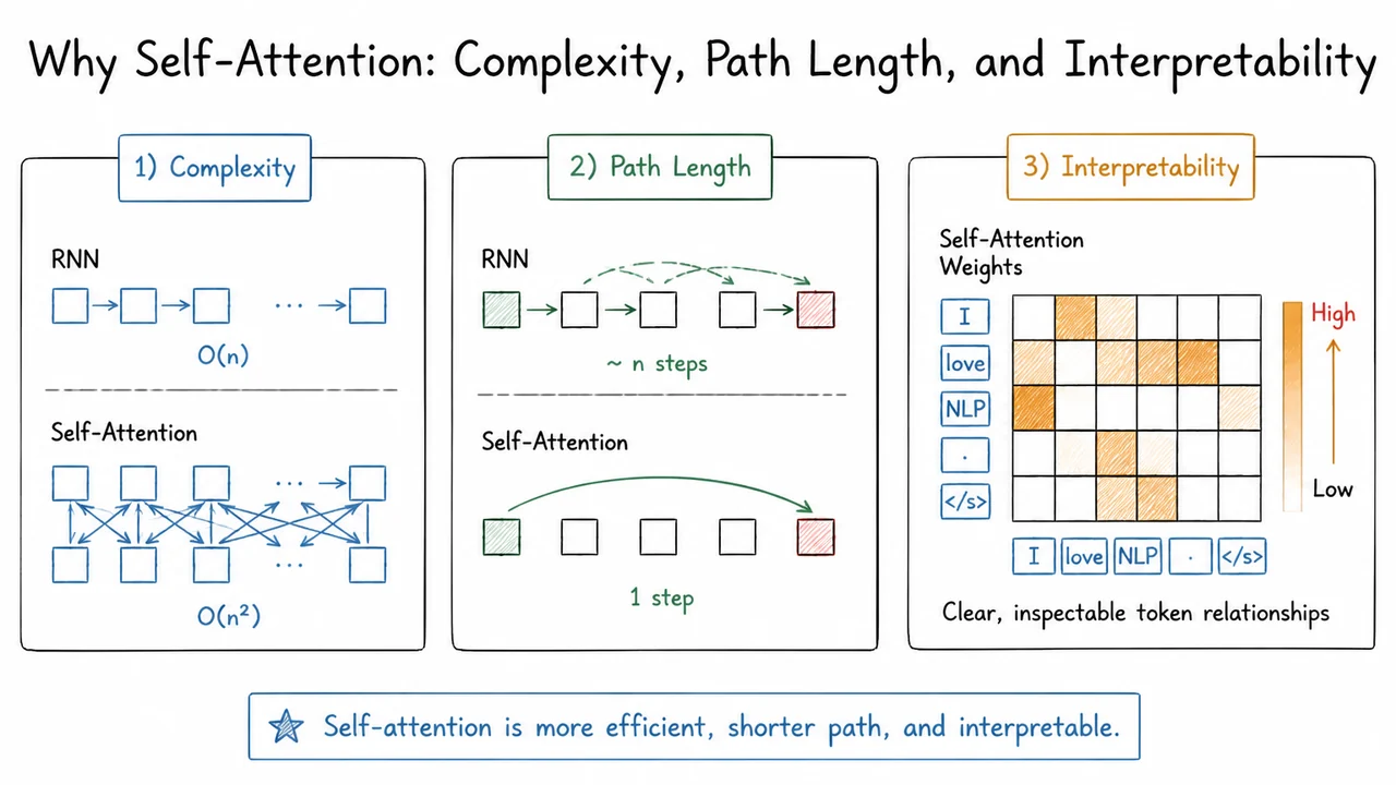
The asymptotic advantages of self-attention are only part of the story. A mechanism with short gradient paths and parallel computation still has to be trained on real data with sensible batching, tokenization, and hardware choices. The original Transformer results therefore depend heavily on a concrete training recipe: large bilingual corpora, subword vocabularies that keep the output vocabulary manageable, length-aware batching that avoids wasted padding, and a multi-GPU schedule that makes the full training run feasible. These details are easy to overlook, but they strongly influence both final translation quality and the practical cost of reproducing the model.
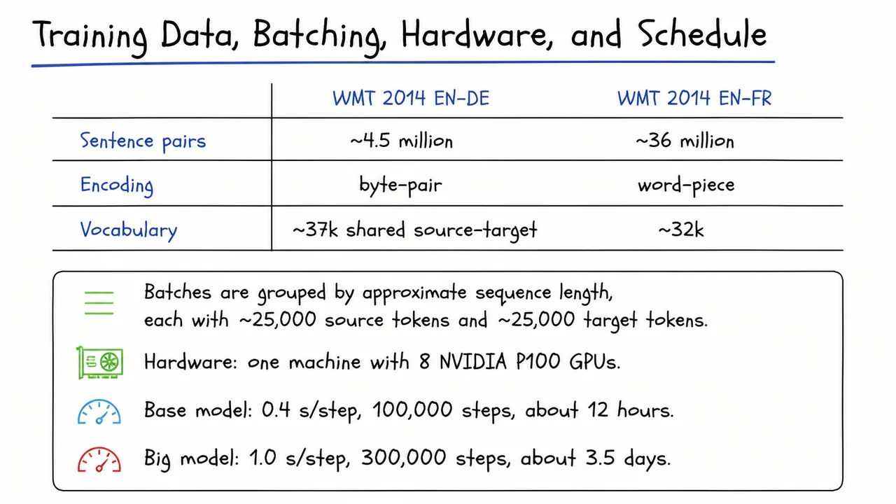
The paper uses two standard machine translation benchmarks. WMT 2014 English-German contains roughly million sentence pairs, while WMT 2014 English-French is substantially larger at about million pairs. The difference in corpus size matters because it changes how much repeated exposure the model gets to rare words and constructions. For English-German, the source and target languages are encoded with byte-pair encoding and share a vocabulary of roughly token types. For English-French, the training setup uses word-piece encoding with a vocabulary of about types. Both methods are subword segmentation strategies: frequent character sequences are merged into larger units, so common words remain whole, while rare or unseen words can be represented as sequences of smaller, more frequent pieces. This avoids the impossible task of predicting over a huge open vocabulary and gives the model a tractable output softmax.
The distinction between byte-pair and word-piece encoding is less important than what they have in common. Both let the Transformer represent morphological variants, compounds, and rare terms without resorting to a fixed word list. The shared English-German vocabulary is a further design choice: source and target subword units come from a common inventory, which simplifies embedding storage and can make cross-lingual parameter sharing more natural. The English-French vocabulary is somewhat smaller but still subword-based, reflecting the different trade-off between coverage and output-layer cost. In both cases, the vocabulary size directly controls the final projection matrix before the softmax, so keeping it around k to k tokens is a practical compromise between expressiveness and computational expense.
Once the data are tokenized, the next operational question is how to form minibatches. The Transformer does not use a naive fixed number of sentences per batch. Instead, it groups examples by approximate sequence length, with each batch containing about 25,000 source tokens and 25,000 target tokens. This length-based token budget is important because sequences in a translation corpus vary widely in length. If batches contained a fixed number of sentences, short sentences would leave most of the padded positions empty, while long sentences could exceed GPU memory. Grouping similar lengths and measuring the batch size in tokens rather than sentences keeps the amount of actual computation more uniform across steps, reduces padding overhead, and stabilizes memory usage.
This batching strategy interacts with the Transformer’s self-attention cost. Because attention is computed over all positions, memory grows with the square of the padded sequence length within each batch. Careful length grouping helps reduce the maximum padded length, but the quadratic cost is still present. The practical success of the Transformer therefore depends not only on asymptotic path length but also on keeping sequence lengths within a manageable range during training. The use of a token budget around k per side is not a universal constant; it is an engineering choice tuned to the available hardware and the typical sentence lengths in the WMT data.
The hardware schedule is equally concrete. Training was performed on one machine with 8 NVIDIA P100 GPUs. The base model ran at approximately seconds per training step for steps, giving a total training time of about 12 hours. The big model ran at about second per step for steps, roughly 3.5 days. These numbers encode both the per-step cost and the total optimization budget. A larger model is not only slower per step because of its greater width and depth, but it is also trained for more steps in the original recipe. Under an 8-GPU data-parallel setup, the effective throughput is much higher than a single-GPU baseline, yet the schedule still keeps the full experiment within a few days on a single machine.
The practical lesson is that Transformer efficiency has two faces: an architectural face, where self-attention allows parallel computation over sequence positions, and an operational face, where batching, tokenization, and hardware scheduling make that parallelism usable. A recurrent model with the same token budget might have required substantially more wall-clock time because of its sequential encoder, while a convolutional model might need careful depth tuning to achieve comparable path length. The stated training recipe makes the architecture’s advantages tangible: even the large Transformer can process hundreds of thousands of update steps in a few days on eight P100 GPUs.
The visual summary below consolidates these operational choices into two clear groups. The top portion of the figure compares the two WMT datasets across sentence-pair count, encoding strategy, and vocabulary size, making the data-level differences immediately visible. The lower portion collects the run-level settings: length-based batching with k source and target tokens, the 8-GPU P100 machine, and the base versus big step times and total durations. This separation is useful because dataset design and training schedule are controlled at different stages of an experiment. The table turns a scattered list of configuration values into a compact mental model: first choose the data representation, then choose how much compute and time to spend.
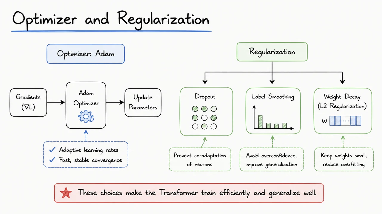
Once the data pipeline, batch size, hardware placement, and step budget are fixed, the next levers that determine whether the Transformer actually converges are optimizer configuration and regularization. These choices are not cosmetic. Transformers have very different optimization geometry from recurrent or convolutional networks: attention layers mix normalized dot products, residual paths create many parallel shortcut paths, and the same weight matrices are used across many token positions. The original Transformer therefore uses a deliberately narrow training recipe rather than a generic deep-learning default.
The base optimizer is Adam. Adam maintains exponential moving averages of the gradient and its elementwise square,
and then updates each parameter with an adaptive step size proportional to . In Vaswani et al., the hyperparameters are , , and . The first moment is standard, but the second-moment decay is slightly smaller than the common . That gives the optimizer a somewhat shorter memory of past squared gradients, which can make it more responsive to rapid changes in the loss surface during the early, high-variance phase of attention training. The very small epsilon is a numerical guard rather than a meaningful damping term; it prevents division by zero without washing out small but informative gradients.
The learning-rate schedule is even more important than the exact Adam constants. The paper uses
with . This schedule has two regimes. For the first 4000 steps the learning rate increases linearly, because the second term inside the minimum is smaller than the first. After that point it decays proportionally to . The overall scale is reduced by , so wider models use a correspondingly smaller base rate. That scaling is not just a numerical convenience; it reflects the fact that attention logits and feed-forward activations grow with hidden width, and a wider model needs smaller parameter updates to change the output distribution by the same amount.
The warmup phase is often the difference between a smooth loss curve and early divergence. At initialization, the combination of random projections, unscaled attention logits, and large embedding tables can produce gradients whose individual coordinates point in very different directions. Adam normalizes by the running second moment, but if that second moment is still small, the first few steps can still be destructively large. Linear warmup lets the optimizer build reliable estimates of gradient scale before the full learning rate is applied. The later inverse-square-root decay is a common stochastic-optimization schedule; it enables large early progress and then a long, stable tail. Removing warmup or increasing the initial rate often causes sudden loss spikes in the first thousand steps.
Regularization in the Transformer is concentrated in two places: residual dropout and label smoothing. Dropout with rate is applied to the output of every sublayer before that output is added back into its residual connection. Concretely, a sublayer computes
so the residual path itself occasionally passes through an identity-like stochastic mask. Dropout is also applied to the sum of the token embeddings and sinusoidal positional encodings. This is a subtle but important choice: the residual stream is the main information highway of the Transformer, and injecting dropout there prevents individual sublayers from becoming irreplaceable. It also acts like a stochastic-depth regularizer without actually dropping whole layers.
Label smoothing changes the target distribution rather than the architecture. Instead of training with a one-hot target that puts all probability mass on the correct next token, the model is trained with a mixture of the hard target and a uniform distribution over the vocabulary, using smoothing value . The loss becomes
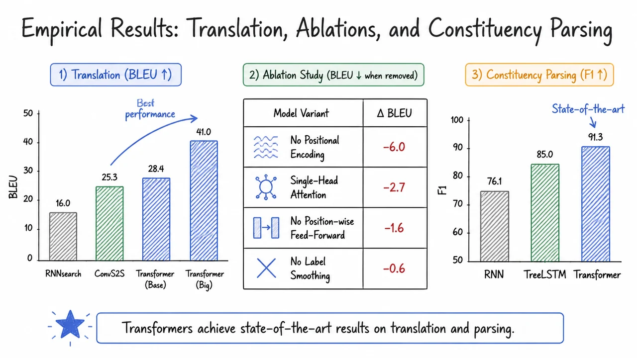
where is a uniform prior over possible tokens. This discourages the model from driving the logit of the correct token toward infinity while forcing all other logits to zero. In practice, label smoothing often worsens raw perplexity because the model is deliberately less confident, but it improves translation quality, as measured by BLEU, and makes the resulting probabilities better calibrated. It also changes the geometry of the output logits so that the model must learn meaningful ranking among many plausible tokens instead of collapsing to a single hard prediction.
These pieces interact. Dropout and label smoothing both add gradient noise and reduce overconfidence, which changes how quickly the loss can be reduced. The warmup and inverse-square-root schedule gives the optimizer enough time to work through that noisier early landscape. If the learning rate is too aggressive, the regularizers cannot prevent overfitting; if dropout is too high, the model may underfit even with a long schedule. The base Transformer recipe is therefore a coupled system: Adam with , warmup for 4000 steps, residual dropout