In the last few years, learned visuomotor policies have achieved something remarkable: they can reliably fold laundry, open doors, and manipulate objects directly from pixel inputs, often exceeding 80–90% success on tasks that once seemed out of reach. Systems like ACT and Diffusion Policy, trained on small batches of human demonstrations, produce smooth, dexterous trajectories that handle variability in object positions and lighting. This progress has rightfully captured the spotlight, yet a quieter problem has been growing alongside it—these policies are simply too slow for real-world deployment. A robot that succeeds but takes a minute to complete a task that a human does in seconds is not a usable system; it’s a proof of concept.
The speed gap can be startling when you compare raw numbers. Take a mundane household task: folding a T-shirt. A person can pick up, fold, and stack a shirt in about 10 seconds. A state-of-the-art robot, running a diffusion-based action chunking policy at its default inference frequency, might take 60 seconds or more. That’s a 6× slowdown. However, this isn’t an isolated quirk of shirt folding. Similar ratios appear across a range of manipulation benchmarks—opening a door, picking an object from a cluttered bin, inserting a peg—where the robot is consistently 5–10× slower than human demonstrators. The high success rates we celebrate are measured in an essentially unlimited time budget, but the real world demands more.
Speed is not a luxury metric; slow execution introduces subtle but pernicious failure modes that undermine the policy’s own competence. When a robot arm moves at a fraction of the speed at which the demonstration was collected, it spends much more time in intermediate states that were barely visited during training. This distribution shift can cause small motion errors to accumulate, leading to motion drift—the arm gradually veers off the intended trajectory and either misses the target or collides with the environment. Moreover, long execution times mean that visual observations used for closed-loop control become stale. If a policy ingests an image at step , takes half a second to compute an action, and then executes that action slowly, the scene may have changed significantly by the time the gripper arrives. The feedback loop that should stabilize the policy becomes sluggish, amplifying perturbations rather than damping them.
There is also a human-centered dimension. For robotic assistants to gain acceptance in homes, hospitals, or factories, they must operate at a pace that feels natural and safe. A robot that folds a shirt with glacial deliberation will not be tolerated by an impatient user, regardless of how perfectly it eventually completes the task. User studies in human-robot interaction consistently show that perceived competence drops sharply when execution speed lags behind human expectations. So speed directly impacts not just technical success but practical adoption.
The core question then becomes: How can we make learned policies fast while preserving their success rate? Simply increasing the control frequency of existing architectures doesn’t solve the problem. Most current policies generate chunked actions over a horizon, then pause to re-infer. The computations required—sampling from a diffusion model, running a transformer decoder many times per chunk—are heavy enough that they impose a minimum latency per decision step. Accelerating the hardware or compressing the model helps, but the fundamental bottleneck often lies in the discrete, piecewise-constant nature of the action representation itself. The policy outputs a sequence of waypoints separated by tens or hundreds of milliseconds, and the robot must interpolate between them at a low level, which can’t capture the fine velocity and acceleration profiles needed for fast, dynamic motion. This is where we start looking for an alternative representation that can compress demonstrations into a continuous, low-dimensional curve—one that a high-frequency controller can execute without waiting for the next neural network inference.
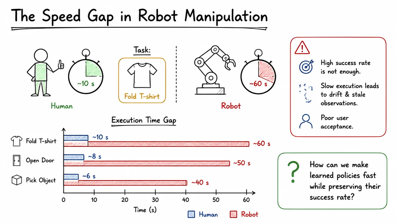
To make the speed gap concrete, let’s lay out a representative comparison. Imagine three manipulation tasks—folding a T-shirt, opening a door, and picking a small object from a table—and measure the end-to-end execution time for a human and for a robot running a diffusion-based policy. The raw numbers are sobering: the human takes roughly 10, 4, and 2 seconds respectively, while the robot takes 60, 25, and 12 seconds. The slowdown factor isn’t uniform; it’s worse for tasks requiring coordinated, continuous motion like folding, but it’s always at least 5×.
The visual that accompanies this section crystallizes that data. It places a human icon and a robot arm side by side, each with a stopwatch, contrasting the folded T-shirt times: ~10 seconds versus ~60 seconds. Below that, a horizontal bar chart arrays the three tasks along the y-axis. For each task, a short blue bar shows the human time, and a long red bar—stretching 5 to 6 times further—shows the robot’s time, with numeric labels on the x-axis. The red bars dominate the chart, and the visual impression is immediate and visceral: robot execution is stuck in slow motion. That chart doesn’t just report numbers; it frames the entire motivation for rethinking how we represent and schedule actions. It’s a graphic reminder that success rate alone is a dangerously incomplete metric, and that the next generation of learned policies must close this speed gap if they are ever to leave the lab.
The previous section made it clear that robot manipulation is hitting a speed wall: real‑world tasks increasingly demand cycles well below 100 ms, yet common learned policies struggle to keep up. A natural first impulse is to ask whether we can simply accelerate the existing policy inference loop: run the same neural network faster, maybe with a smaller model, and call it a day. That fails because the bottleneck is not only computation but also the representation of actions. If the policy produces a rigid, discrete sequence of commands, speeding up the clock will expose fundamental structural weaknesses that were invisible at leisurely demonstration speeds. The real culprit is the ubiquitous discrete action chunking paradigm, and its two core limitations—uniform temporal resolution and chunk discontinuities—are what we must dismantle before we can design a policy that truly flies.
In the standard action‑chunking setup, a policy conditioned on a short window of observations predicts a fixed‑length block of future actions: where is the action horizon, typically something like 16, 32, or 64 steps. These actions are executed open‑loop in order, and the next prediction cycle starts exactly at time . The representation is intuitive and easy to train via behaviour cloning, but it forces a strict, uniform sampling of the timeline. Every consecutive step inside a chunk lives at the same interval , and the policy can only influence the future at those pre‑defined, equally spaced instants.
The first limitation is the uniform temporal resolution. A block‑stacking task, for example, contains phases with dramatically different dynamics: a free‑space reaching motion might need only a handful of coarse waypoints, while the delicate insertion or contact‑rich aligning phase demands dense, high‑frequency feedback. Discrete chunks paint every task phase with the same brush—if is chosen to accommodate the finest manipulation, the reaching phase is littered with redundant, unnecessarily fine‑grained commands that waste representation capacity and can even introduce high‑frequency jitter. Conversely, a coarse that suffices for reaching will under‑sample the contact phase, losing the subtle force‑modulation cues that make the difference between success and failure. The representation has no mechanism to adapt its sampling density to the needs of the task.
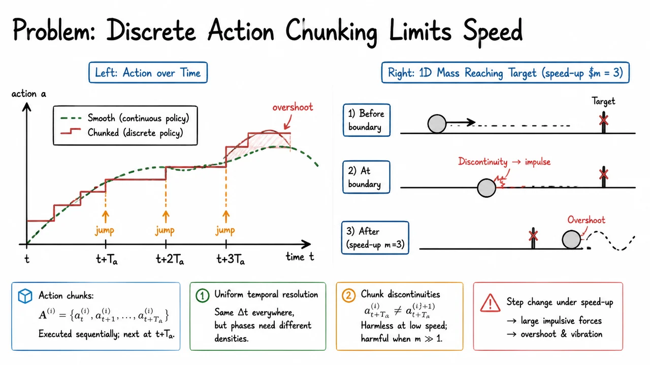
The second limitation, and the one that turns catastrophic under speed‑up, is chunk boundary discontinuities. Each action chunk is predicted independently from the next chunk , conditioned on the observation at its own starting timestep. Because the world evolves while the chunk executes, and because the policy is stochastic or simply imperfect, there is no guarantee that the final action of one chunk will match the first action of the next. Formally, almost surely. At the nominal demonstration speed this mismatch is small enough that a robot’s low‑level controller and the natural damping of the manipulator smooth it out. The commanded position, velocity, or torque changes by a tiny amount that the servo loop absorbs without complaint. But as we push the policy to run m‑times faster by scaling the time‑base (), that tiny positional or velocity jump transforms into a large impulsive change. The step discontinuity now arrives as a sharp velocity command or a sudden torque spike. The effect on a physical robot is immediate: overshoot, ringing vibrations, and even hard mechanical shocks that can damage hardware or knock objects out of the gripper.
A revealing mental model is a simple point mass trying to reach a target position under position control. A smooth, continuous policy—like a carefully fitted curve—glides the mass directly to the goal. Now replace that with a stair‑step action signal that updates only at chunk boundaries. When played back at normal speed, the steps are small and the mass settles softly. Speed up the trajectory by a factor of , however, and each step becomes a sudden jump that the mass cannot follow without overshooting; the discontinuity injects an impulse that sends the mass past the target, forcing the policy to correct in the next chunk, often leading to oscillatory failure. The same reasoning holds for a multi‑joint arm: boundary jumps multiplied by speed‑up become large unintended forces that the underlying controller must fight, destroying both accuracy and execution smoothness.
These two problems—static resolution and boundary jumps—are deeply linked. Uniform temporal resolution forces the policy to waste capacity on simple phases while starving complex phases; chunk discontinuities inject energy into the system at every policy update. Together they set a hard ceiling on how fast a discrete‑chunk policy can move before its own representation sabotages performance. Any attempt to achieve high‑speed manipulation by simply shrinking the action horizon or running the inference loop more frequently still leaves the fundamental discontinuity issue, and may worsen the resolution mismatch.
The visual below captures this pathology in a compact side‑by‑side analysis. The left panel plots a desired smooth trajectory (dashed green) against the stair‑step output of a discrete‑chunk policy (red). Orange arrows flag the boundary jumps where fails to connect to , and a light shaded region highlights the overshoot that follows. The right panel brings the 1 D point‑mass analogy to life: three snapshots show the mass overshooting the target flag because of the discontinuity injected at a speed‑up factor of . The annotations “Discontinuity → impulse” and “Overshoot” make the causal chain explicit: the step change at the chunk boundary becomes an impulse that the mass cannot damp quickly enough, leading to failure. This one‑dimensional cartoon is not just a pedagogical toy—it isolates the exact mechanism that, in a high‑speed manipulation setting, turns a decent policy into a vibrating, imprecise, and potentially dangerous controller.
Thus, if we want robotic policies that are both fast and dexterous, we must abandon the idea that actions should be delivered as independent, uniformly‑spaced chunks. The next section introduces a paradigm shift: replacing these discrete stair‑steps with a continuous action curve that naturally handles variable task density and eliminates boundary discontinuities entirely.
The previous section identified a core friction in behavior cloning pipelines: naively predicting a fixed-length sequence of discrete actions forces the policy to commit to a uniform temporal grid. This constraint produces jerk at chunk boundaries, wastes representational capacity on redundant samples, and makes it cumbersome to change execution speed without distorting the learned behavior. To overcome these limitations, we need to replace the idea of a sequence of waypoints with a parametric curve that represents actions continuously over time. This is not merely a cosmetic change; it fundamentally decouples the action representation from the execution clock and unlocks new axes of smoothness, scalability, and local adaptability.
The central object in this paradigm shift is the action curve , a mapping from a normalized time coordinate to the action space of the robot. Instead of predicting individual action vectors at discrete timesteps, the policy now outputs a compact description of the whole curve. A natural and powerful family of continuous functions for this purpose is the B‑spline (basis spline). A B‑spline curve is defined by three ingredients: a set of control points in the action space, a degree that controls smoothness, and a knot vector that partitions the parameter domain. The curve itself is a weighted sum of locally supported basis functions :
The basis functions are computed recursively from the knot vector and are non‑zero only over a small interval, so each control point influences the curve only in its immediate neighbourhood. This local support is the mathematical engine behind the B‑spline’s attractive control properties, while the degree guarantees that the curve is continuous (assuming uniform knots away from endpoints). For common choices such as cubic splines (), this yields smoothness—continuity of position, velocity, and acceleration—which is impossible with discrete waypoints.
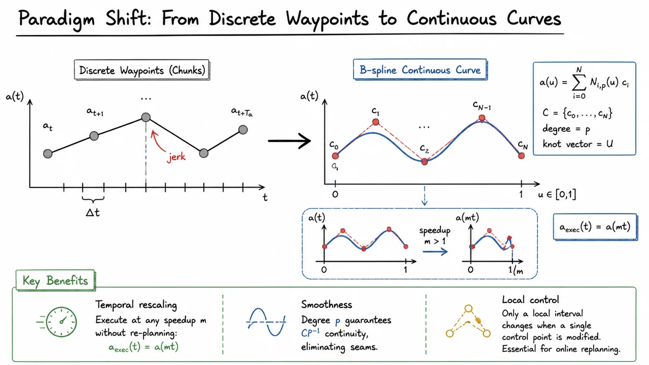
Why does this representation matter so much for robot manipulation? First, it provides temporal rescaling as a first‑class operation. Because the action curve is a continuous function of the abstract parameter , we can map it to real execution time via any monotonic scaling . The executed action becomes , where the speedup factor compresses or dilates the motion without altering the shape or physical feasibility of the path. A policy trained on demonstrations at normal speed can thus be deployed at a much faster rate simply by increasing ; there is no need to retrain, reparameterize, or risk introducing artifacts like chunk‑stitching jerks. This clean separation between what to do (the curve) and how fast to do it (the time warping) is a profound engineering advantage.
Second, the smoothness inherent in the B‑spline representation directly eliminates the jerk problem. Discrete action chunking stitches together linear or zero‑order holds, creating velocity and acceleration discontinuities at every chunk transition. A degree‑ B‑spline, in contrast, is continuous across the entire domain. For a cubic spline, this means that both the command signal and its first two derivatives are continuous, leading to naturally fluid motion even when we later sample the curve at an arbitrary frequency. There are no hidden seams to manage, and the robot controller receives a consistently filtered trajectory that respects its torque and jerk limits.
Third, local control enables efficient online replanning. If the robot encounters an unexpected obstacle or a target moves, we can update only a single control point to adjust a localized section of the trajectory. The change propagates only along the knot spans touched by that basis function, leaving the rest of the curve untouched. This contrasts sharply with discrete representations, where modifying one waypoint can cause a ripple of corrections across adjacent points to maintain smoothness. Local control makes it computationally cheap to perform incremental refinements, an essential capability for reactive, closed‑loop policies.
The B‑spline equation also clarifies the compactness of the representation. While the raw demonstration may contain hundreds of high‑frequency samples, the underlying trajectory can often be encoded with a small set of control points—often 8 to 20 for a manipulator arm motion. The policy learns to output these control points (and, if needed, a knot vector) directly, drastically reducing the output dimension compared to predicting a long sequence of action vectors. This condensed output is easier to supervise, generalizes better, and leaves room for the policy to focus on the shape of the motion rather than redundant timing details.
The visual below concretizes this contrast by pitting the two worlds against each other. On the left, a discrete action chunk appears as a staircase of grey waypoints connected by linear segments; a sharp red arrow marks the inevitable jerk at a chunk boundary, while uniform tick marks on the time axis underscore the rigidity of a fixed . On the right, the same underlying motion is expressed as a smooth cubic B‑spline: a blue curve glides past red control points, and a dashed red control polygon hints at the underlying structure. An inset panel then drives home the temporal rescaling insight: the very same control points are plotted against a compressed time axis (scale factor ), producing an identical spatial shape squeezed horizontally, with clear labels and to cement the mapping. This side‑by‑side layout makes tangible how the B‑spline approach replaces jerky, rigid chunks with a fluid, time‑flexible representation that is ready for high‑speed execution.
To appreciate why a paradigm shift is necessary, it helps to look at the earlier generation of methods that attempted to make robot policies run faster. In high‑speed manipulation tasks—think of flipping a pancake, catching a moving ball, or dynamic peg insertion—even a policy with flawless accuracy becomes useless if its action stream cannot be replayed at the required physical cadence. The naive solution is to reduce the latency between action decisions, but simply generating the same set of waypoints at a higher frequency does not produce smooth motion; it merely replays a coarsely sampled trajectory faster, with all the stuttering and overshoot that come from chaining discrete poses at larger time steps. Researchers have attacked this problem from several angles, yet a common limitation remains: all prior acceleration techniques tinker with how or when discrete actions are emitted, without ever questioning the discrete action representation itself.
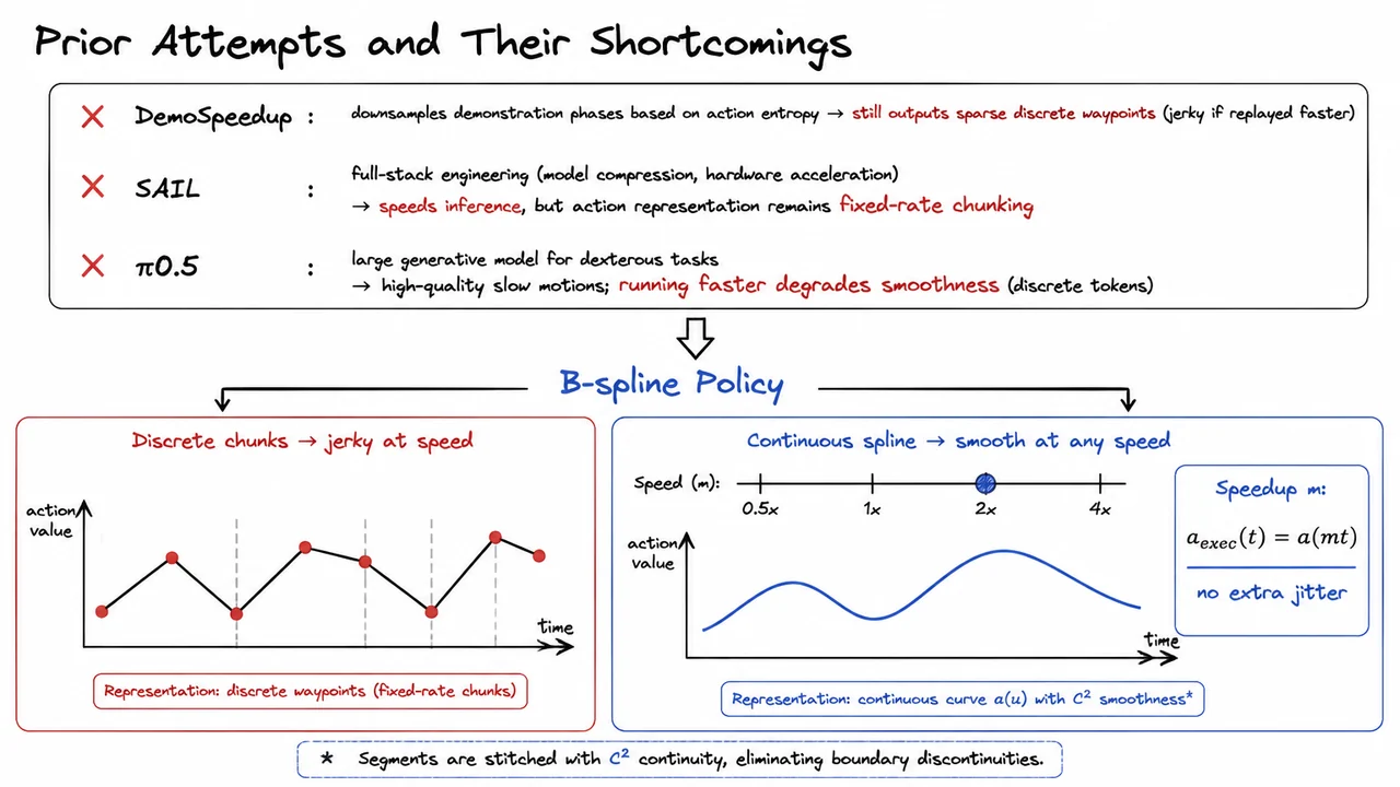
The first notable approach, DemoSpeedup, focuses on compressing demonstration trajectories by non‑uniformly downsampling them based on action entropy. The idea is elegant: during slow, low‑entropy phases (e.g., holding a steady pose), you can safely skip many intermediate waypoints. The resulting sparse sequence still captures the salient poses and, when replayed at normal speed, appears faithful. However, DemoSpeedup still outputs a sequence of discrete waypoints—fewer of them, but still discrete. When the user now accelerates playback by a factor , the controller simply steps through those waypoints at times the original rate, linearly interpolating between them. Because the original spacing was optimized for a different temporal scale, the accelerated motion becomes jerky: the robot lunges from one sparse key pose to the next, losing the subtle acceleration profiles and continuous curvature that made the demonstration smooth. In essence, DemoSpeedup trades speed for spatial fidelity, and the trade‑off deteriorates rapidly as grows.
A second line of work, exemplified by SAIL, attacks the problem from the hardware and inference side. Here the goal is to reduce the model’s execution time through full‑stack engineering: model compression, quantization, hardware‑aware kernel design, and off‑loading to dedicated accelerators. A faster model can produce the same chunk of discrete actions at a higher inference rate, thereby reducing the per‑chunk latency. This genuine engineering achievement makes it possible to run complex policies in real time on resource‑constrained platforms, but it does not alter the nature of the action stream. SAIL still outputs a fixed‑rate chunk: a block of, say, 10 waypoints to be consumed over the next 100 ms. Speedup up by increasing the replay rate means the same chunk must be played back over a shorter horizon, forcing the controller to interpolate between the same number of points in less time. The result is higher instantaneous velocities and, more critically, sharp discontinuities at chunk boundaries where the next chunk arrives with a slightly different predicted pose. The representation itself is the bottleneck, not the inference speed.
A third, more recent effort is π0.5, a large generative model that produces entire action sequences for dexterous tasks. At standard speed, π0.5 generates remarkably fluid motions because the model can attend to a long horizon. Yet when one tries to accelerate execution, a new failure mode appears: the underlying token sequence of the generative model is discrete. Speeding up playback forces the token decoder to run in a time‑compressed regime, where the same number of generated action tokens must cover a smaller real‑time window. Because the model’s internal dynamics were not trained to maintain smoothness under temporal compression, the result is a degradation of motion quality—vibration, overshoot, or even physically inconsistent commands. Here, too, the discrete token representation itself throttles what acceleration can achieve.
What do DemoSpeedup, SAIL, and π0.5 share? Each modifies the process of generating discrete actions—by temporal downsampling, inference acceleration, or model scaling—but none escapes the fundamental constraint: the policy’s output is a finite set of waypoints whose spacing is fixed at design time. The moment you alter the playback speed, you are forced to interpolate or extrapolate from those waypoints, introducing jitter, boundary discontinuities, or temporal artifacts. In other words, the smoothness of the resulting motion is inseparably coupled to the execution speed, and that coupling is hard‑wired into the discrete action representation.
The B‑spline Policy breaks this coupling by changing the representation itself. Instead of a list of waypoints, the policy emits the parameters of a continuous action curve —a parametric path in the robot’s joint or end‑effector space that is guaranteed to be at least smooth. Once you have such a curve, speeding up execution by a factor becomes trivial and lossless: you simply evaluate the curve at a temporally scaled parameter, . There are no new interpolation points to invent, no chunk boundaries to align; the underlying geometry of the motion is preserved exactly, and the curve’s smoothness guarantees jerk‑free motion at any speed. Moreover, when the policy generates a sequence of spline segments, they are stitched together with continuity, so the transition from one segment to the next introduces no abrupt acceleration jumps—something impossible with discrete waypoint lists.
The visual below distills this contrast. The upper portion calls out the three prior methods with subtle red cross marks, underscoring that each eventually succumbs to the jerky‑speed trade‑off because they leave the discrete representation unchanged. The lower part then juxtaposes the two worlds: on the left, a sequence of discrete waypoints connected by jagged line segments—the inevitable result of chunk‑based replay at high speed; on the right, a smooth blue spline with a simple speed slider mapping the factor directly to the curve’s parameterization. The slider visualises the idea that is all you need—and that continuity stays intact regardless of . This side‑by‑side comparison crystallises the core insight: only a continuous action representation can decouple the quality of motion from the execution speed. All prior attempts speed up the delivery of discrete actions; the B‑spline policy, in contrast, delivers a curve that inherently carries its own smooth geometry, ready to be traversed at any rate.
Up to this point, we have seen that discrete action chunking struggles at the edge of high-speed manipulation: chunks introduce fixed latencies, boundaries create discontinuities, and the robot’s execution clock can easily diverge from the policy’s asynchronous stepping. The core tension is that a robot arm under real-time control needs a dense stream of setpoints—often at kilohertz rates—yet a learned policy should operate at a much coarser timescale to remain feasible. This tension invites a deeper question: can we repurpose a well-known tool from geometry and CAD to serve as a language for actions, one that is inherently continuous, compact, and predictable?
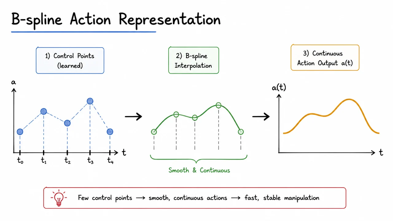
Enter B-spline curves. Instead of having the policy emit a long sequence of individual target poses, we let it emit a small set of control points and a knot vector that together define a smooth, time-indexed trajectory. A B-spline is a piecewise polynomial curve defined over a non-decreasing sequence of knots . Given control points (each a point in the robot’s action space—joint positions, end-effector poses, or a latent embedding), and a degree , the curve is
where the basis functions are defined recursively via the Cox–de Boor formula. The parameter is typically mapped to a normalized time, so evaluating at a specific moment gives the desired action command. This formulation has several properties that make it a perfect match for high-speed manipulation.
First, compactness. A B-spline can represent a complex, long-horizon trajectory with far fewer parameters than a raw sequence of waypoints. For example, a 2-second reach at 500 Hz would otherwise demand 1,000 setpoints; a cubic B-spline with 10–20 control points can reproduce the same path to sub-millimeter accuracy while reducing the output dimension by two orders of magnitude. Second, smoothness. The curve is times continuously differentiable inside each knot span; for (cubic), both velocity and acceleration are continuous, which is critical for minimizing jerk and avoiding saturating motor torques. The robot executes a single flowing motion rather than a series of abruptly stitched micro-actions.
Third, and perhaps most subtly powerful, is local control. Each control point only influences the curve over a limited interval of the knot vector—exactly knot spans. Moving a single control point modifies the trajectory locally without disturbing segments far away. For a policy, this means a small correction or adaptation (say, to avoid a new obstacle) can be made by adjusting one or two control points near the current time, leaving the rest of the planned curve intact. The policy can perform incremental refinement during motion, an ability that discrete chunking fundamentally lacks because altering one state in the chunk can violate continuity with neighbors.
The accompanying visual distills these ideas into a single diagram. It shows a smooth, curved trajectory—drawn in that familiar sketchy style—alongside its control polygon (the dashed lines connecting the control points), which acts as a coarse scaffold. A small cluster of control points is highlighted to illustrate local influence: only the part of the curve near those points changes when they move. Annotated elements call out the knot vector as the temporal spine and the basis functions as the blending weights. The diagram reinforces the central narrative of the B-spline action policy: the policy only needs to predict a handful of control points, and the robot’s controller interpolates this continuous representation on the fly, achieving smooth, reactive, and computationally lightweight execution even at speed. This is not just an alternative parameterization; it is a structural shift from discrete planning to continuous shaping.
Even after a policy generates valid actions, the real challenge in high-speed manipulation is executing those actions at the right tempo without destroying the learned behavior. Standard discrete action chunking—outputting a fixed-length sequence of actions at the policy’s native rate—creates a tight coupling: the inference rate dictates the control loop frequency. If the policy runs at 10 Hz, the robot receives new commands only every 100 ms. Speeding up the task naively by increasing the loop rate simply repeats or interpolates coarse chunks, which introduces jerks and can violate the delicate dynamics the policy was trained to respect. Conversely, training the policy for a higher rate is expensive, often infeasible, and still locks the speed to a single value. We need a representation that decouples the action description from the execution schedule—and that is exactly where B‑splines excel.
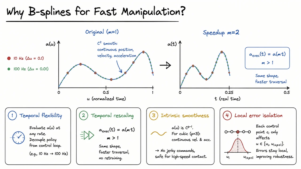
A B‑spline policy outputs a continuous action curve defined on a normalized time parameter , not a discrete array of steps. This curve is a weighted sum of smooth basis functions (typically cubic for manipulation) controlled by a small set of control points. Because the representation is inherently continuous, we can evaluate at any desired rate on the robot controller, completely independent of how often the policy produced the curve. This property—temporal flexibility—breaks the old coupling. A policy generating a new curve at 10 Hz can still feed a 100 Hz control loop: the controller simply samples at 100 equally spaced points along inside each policy interval. The curve’s shape remains intact, but the actuation density is now matched to the robot’s high-frequency needs.
Temporal flexibility is only half the story. Naively sampling a fixed curve more densely does not make the motion faster—it only reduces the temporal gaps between commands. To change execution speed without altering the trajectory’s geometric or dynamic shape, we exploit temporal rescaling. Because the B‑spline action is a function of normalized time, we can accelerate the whole movement uniformly by simply warping the time axis. Given a speed multiplier , the executed action becomes where is the real clock time elapsed from the start of the current action segment. The result is the identical action shape traversed times faster. Critically, this transformation requires no retraining, no adjustment of control points, and no extra data. The same policy that works at 1× speed can instantly operate at 2× or 1.5×, preserving smoothness and task semantics.
Smoothness itself is not a cosmetic bonus; it is a physical necessity for fast manipulation. Abrupt changes in commanded position or velocity cause large jerk, excite high-frequency vibrations, and can break contact with the environment—all catastrophic for tasks like high‑speed insertion or flipping. B‑splines built with cubic basis functions () guarantee continuity, meaning position, velocity, and acceleration are continuous across the entire curve. There are no discrete jumps hidden in the action sequence. The robot receives a flow of commands that respects second‑order continuity, making high‑speed trajectories safer and more predictable.
A fourth property that solidifies the robustness of the B‑spline policy is local error isolation. In a discrete sequence, a single corrupted action frame can propagate errors through temporal averaging or feedback loops. With B‑splines, each control point influences the curve only over the parameter interval a limited local domain. If the policy mispredicts one control point, the distortion is confined to a short segment of the action; the rest of the curve remains unchanged. This locality also makes it easier to correct or adjust portions of the trajectory online without recomputing the whole curve—an advantage for reactive manipulation.
The combination of these four attributes—temporal flexibility, temporal rescaling, intrinsic smoothness, and local error isolation—transforms how we think about action generation for fast manipulation. They collectively attack the speed bottleneck not by asking the policy to run faster, but by changing the shape of the problem: the policy produces a compact, smooth, re‑parameterizable action curve that the robot can render at any desired rate and speed.
A side‑by‑side visual snapshot consolidates these ideas. On the left we see the same smooth B‑spline action trajectory over normalized time from 0 to 1. Sparse red markers show what a 10 Hz policy would naively command, while dense green markers show the 100 Hz evaluation points the robot controller can extract from the exact same curve—illustrating arbitrary sampling rates without altering the underlying action. On the right, the same curve is plotted under temporal rescaling with (i.e., ) against the real time now spanning only 0 to 0.5 seconds. The shape is preserved identically, compressed horizontally, driving the robot through the same motion in half the time. A floating annotation near the curve highlights its smoothness—continuous position, velocity, and acceleration—reinforcing why the transition to high‑speed control remains graceful. This compact graphical comparison makes the message immediate: B‑splines free the policy’s output from the shackles of a fixed execution rate, enabling on‑the‑fly speed changes and smooth, high‑frequency control without ever revisiting the policy network.
If you’ve internalized why B‑splines are a natural choice for representing robot action curves—continuous differentiability, local support, and a compact parameterization—the next practical challenge is how to actually go from a raw demonstration trajectory to an efficient B‑spline target. A human demonstrator often produces a dense sequence of time‑stamped poses or joint commands:
where can be hundreds or thousands, yet we want a representation that can be evaluated quickly during closed‑loop control and that doesn’t bloat the policy’s output space. The fitting problem is to find a degree‑ B‑spline curve
that approximates while keeping the number of control points as small as possible—ideally far smaller than . This is a delicate balance: an overly parsimonious spline will smooth out sharp turns and violate the accuracy requirement, whereas a spline that matches every demonstration point exactly is just a re‑parameterization of the raw data, offering no compression.
The first step is to align the time stamps with the B‑spline’s natural parameter domain, typically . We map each original time to a normalized parameter
so that the sequence falls into the unit interval. Because the speed of the demonstration may vary, the are not necessarily uniformly spaced—some regions will be densely sampled, others sparser, but the spline must represent the overall shape faithfully.
We then define the reconstruction error as the maximum Euclidean distance between the spline evaluation at each data parameter and the recorded action:
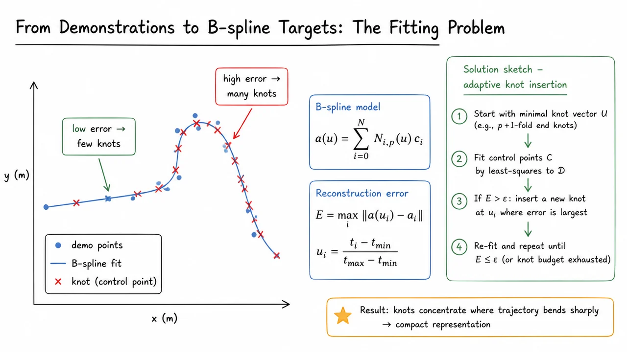
The constraint for a user‑defined tolerance guarantees that the fitted curve never deviates from any demonstration point by more than . Since is a linear combination of B‑spline basis functions, for a fixed knot vector and degree the control points that minimize a squared‑error loss can be found via a straightforward least‑squares solve. However, starting with a minimal knot vector (often only the ‑fold end knots so that the curve is a single Bézier‑like segment) will almost certainly violate the error bound if the demonstration contains sharp corners or high curvature.
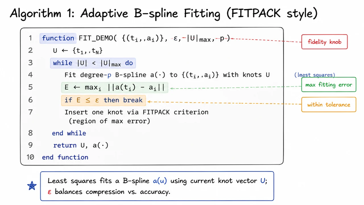
This is where adaptive knot insertion comes into play. The algorithm follows a FITPACK‑style loop: begin with the minimal knot vector; solve for the control points that best fit the data in the least‑squares sense; compute and locate the data parameter where the largest deviation occurs. If , insert a new knot exactly at , update the knot vector, and re‑fit. Repeating this process steadily reduces the error, because adding a knot increases the flexibility of the spline precisely where it is needed most. The loop terminates as soon as or a maximum knot budget is exhausted, yielding a compact B‑spline that satisfies the tolerance.
The beauty of this approach is that knots naturally concentrate where the trajectory bends sharply—high curvature demands more basis functions to capture the local shape without overshoot or unacceptable error. Straight‑line segments, on the other hand, can be faithfully represented by a single low‑order polynomial piece, so very few interior knots (often none) are added in those regions. The result is a compact, smooth action representation that respects the geometric complexity of the demonstration and uses its control point budget efficiently.
The illustration that follows captures this iterative, curvature‑aware fitting. In the diagram, the demonstration points trace an end‑effector path with a pronounced sharp turn; the fitted B‑spline curve runs smoothly through the data (up to ). Knot locations are marked with crosses along the trajectory. The visual contrast is stark: the long, almost‑straight segments are adorned with only a handful of knots, while the tight corner is crowded with crosses. Accompanying labels drive home the principle: “low error → few knots” on the linear stretches, “high error → many knots” on the turn. The plot, with its axes in meters showing the spatial interpretation, immediately demonstrates that adaptive knot insertion yields a representation where knot density mirrors curvature, and that the fitted spline is both compact and a faithful proxy of the original demonstration—a perfect symbolic launchpad for the algorithmic details in the next section.
The previous section established that raw demonstration trajectories—lists of timestamped action vectors—cannot be fed directly into a policy that must output smooth, continuous motion. We need a compact functional representation that the B‑spline policy can learn to produce. That representation is a B‑spline curve, but the question remains: how do we choose the knot vector and the control points so that the spline faithfully captures the demonstrated behavior without overfitting every tiny tremor or pause? The answer lies in an adaptive fitting strategy that automatically places more knots where the trajectory is complex and fewer where it is simple, all while respecting a user‑specified tolerance .
Mathematically, we are given a set of data points , where each is a timestamp and is the desired action vector (e.g., joint velocities or end‑effector twists). We want to construct a degree‑ B‑spline function such that the maximum deviation over the timestamps is controlled. Directly optimizing both the control points and the knot vector is a challenging non‑linear problem. Instead, we adopt a classic iterative refinement approach inspired by the FITPACK library: start with a minimal knot vector (only the endpoints and ), perform a least‑squares fit for the control points, measure the worst‑case error, and then add a new knot where that error is largest.
Why least‑squares? Because the demonstration data often contains mild sensor noise or human variability that we do not want to replicate exactly. The B‑spline is a linear function in the control points once is fixed, so fitting becomes a simple, well‑conditioned linear least‑squares problem. Specifically, we solve for the system , where is the matrix of basis function evaluations and contains the stacked target actions. The resulting spline minimizes under the given knot configuration.
The adaptive part is where the real power lies. After each least‑squares fit, we compute the maximum residual If , we have already achieved the required fidelity and we stop; the current knot vector is sufficient. If not, we must add detail where the fit is poorest. The FITPACK criterion selects the interval (or timestamp) where the local error is largest and inserts a new knot—often at the midpoint of that interval or at the timestamp itself, depending on the variant—thereby granting the spline an extra degree of freedom to bend more sharply in that region. This process repeats until either the error drops below or we reach a predefined maximum number of knots to prevent runaway complexity.
This algorithm elegantly balances two competing desires. A tight tolerance yields a curve that hugs the demonstrations closely, but at the cost of a larger knot set and a more expressive policy target that may be harder for the learning system to predict correctly. Conversely, a looser gives a smoother, more compressed representation that can be more robust during inference, but it might smooth out critical motion details. In this sense, is truly a fidelity knob—a single scalar parameter that lets the practitioner dial the trade‑off between compression and accuracy, without hand‑tuning knot placements.
The entire procedure, summarized in the visual below, is compact enough to fit in a dozen lines of pseudocode. The diagram presents Algorithm 1: Adaptive B‑spline Fitting (FITPACK style) as a clean monospaced block. It highlights the while‑loop that drives the iterative refinement, the central error evaluation , and the early‑break condition that exits as soon as the fidelity target is met. A small annotation next to the tolerance reminds the viewer that is the “fidelity knob,” while a footnote beneath the box notes that least‑squares fits a B‑spline using the current knot vector . This compressed visual serves as both a reference for implementation and a conceptual anchor: the entire pipeline from raw demonstration data to a compact, continuous action target is distilled into a single, self‑contained routine that respects the user’s tolerance and computational budget.
With the adaptive fitting algorithm from the previous section, we can distill any demonstration into a sequence of compact B‑spline segments—each one a smooth action curve defined by a handful of control points and a local knot vector. But a neural policy that runs on the robot cannot emit a new segment of arbitrary length; standard network architectures require a fixed‑size output. If we flatten the parameters of a spline whose length varies freely, the tensor shape changes from sample to sample, and supervised learning breaks down. The challenge is to encode a variable‑duration action plan into a constant‑size prediction vector without losing the flexibility that makes B‑splines attractive for high‑speed manipulation.
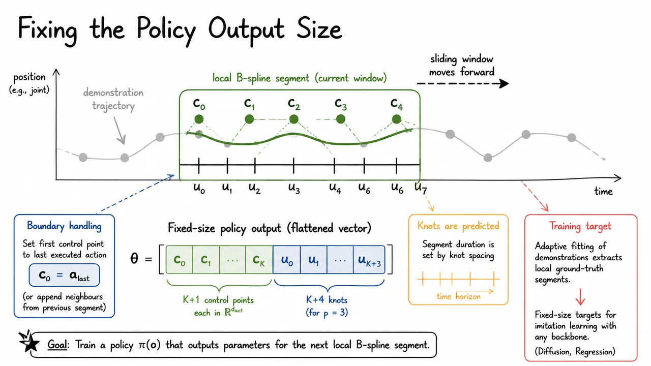
The key to fixing the policy output size lies in the local support property of B‑splines. Recall that a cubic B‑spline evaluated on a single knot interval depends on exactly control points: the shape inside that interval is a convex combination of . If we confine the action segment to a window that spans a few knot intervals—say, intervals—the entire curve within that window is determined by at most knots and exactly control points (because every control point influences at most four intervals, and those wholly outside the window can be ignored). Therefore, by choosing a safe upper bound for the number of control points we ever need, we obtain a constant‑size parameterization of any local trajectory segment, regardless of its actual duration or velocity profile.
In practice, the policy will predict control points (or points, depending on indexing) together with the associated knot vector. The knot positions are not fixed in advance because they encode the time stretching of the segment: a densely spaced knot sequence compresses the curve into a short duration, while sparse knots stretch it over a longer horizon. By making the knots part of the policy output, we let the network decide both the shape and the timing of the action—the segment’s total time‑length emerges from the knot spacing. The flattened output vector then takes the fixed form
where each control point carries the full action dimension (e.g., joint positions or end‑effector poses). This vector always has the same length, even though the resulting curve can cover a vastly different time span depending on the predicted knots.
A delicate boundary condition must be satisfied to stitch consecutive segments seamlessly. The policy’s current prediction should begin exactly where the previous executed segment ended, so the first control point is not freely predicted. Instead, it is set equal to the last executed action (the current robot state). This hard‑wired continuity eliminates the need for a separate blending step and guarantees that the action curve leaves no gap or jump at the boundary. The rest of the control points and all knots are then free to be learned by the policy, forming a smooth continuation of the motion.
Training such a policy uses the adaptive fitting pipeline described earlier (Algorithm 1). For each demonstration, we slide a window of fixed knot span along the recorded trajectory, extract a local B‑spline segment via smoothing spline fitting, and store its parameters as the ground‑truth target . Since the window size in terms of number of control points is constant, every extracted segment becomes a same‑size vector. These pairs —observation to B‑spline parameters—are the training data for any imitation‑learning backbone, be it a plain regression network or a diffusion model. The learned policy is then able to output a fresh local spline segment, ready for immediate execution.
The visual below consolidates this idea. A 2D demonstration trajectory (e.g., a joint position against time) is drawn in grey, fading outside the active window. A highlighted box frames the current local segment within which a green B‑spline curve passes through or near the data, its control points shown as filled dots and its knot positions as vertical tick marks along the time axis. Next to the box, the fixed‑size vector is represented as a sequence of coordinate blocks for the control points followed by the knot values. A dashed arrow indicates the window sliding forward along the trajectory, mimicking the online policy’s step‑by‑step operation. The diagram makes it immediately clear: a constant‑length output vector, built from local support and learned knots, is all we need to generate flexible, variable‑length action curves for fast robotic execution.
Having settled on a compact, fixed-size B‑spline representation for the policy’s output, we can now produce overlapping spline segments at the rate of the inference pipeline. Each segment describes a continuous action trajectory over a time horizon , parameterized by a normalised parameter . Because we forward the network periodically (every seconds) and immediately dispatch the new spline to the low‑level controller, a new segment arrives while the previous one is still being executed. This pipelined dispatch is the key to continuous, uninterrupted motion.
The challenge appears at the switching instant—when the controller finishes playing back the old segment and starts the new one. In an ideal world, the end of the old spline would coincide exactly with the beginning of the new spline, and the velocity profiles would match. In practice, prediction noise, numerical inaccuracies, and the unavoidable inference latency itself (the delay between sensing a state and receiving the new spline) break this perfect stitching. The controller may receive a few milliseconds late, or the network may output a segment whose initial point differs slightly from the true executed state. The result is a boundary discontinuity: a sudden jump in the commanded action that the robot’s actuators try to follow, producing a sharp force transient and potentially destabilising the manipulation. High‑speed contact‑rich tasks are especially unforgiving of such jitter.
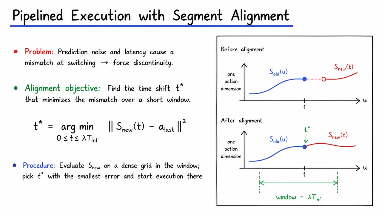
We can think of the mismatch as a temporal misalignment between the new spline and the real execution timeline. The B‑spline’s continuous‑time nature gives us a powerful tool: we are free to start playback at any point along its curve, not necessarily at . If the network’s prediction is off by a small amount in timing—perhaps it intended a certain force profile starting from the moment of observation but actually began later—we can shift the new segment forward in its own parameter space. The question becomes: what is the optimal (real time offset from the beginning of the segment, with ) such that best matches the last executed action ?
Formally, we cast this as a one‑dimensional optimization over a short search window:
The search window is bounded by the inference latency, expanded by a small factor (often around ) to account for jitter and slight estimation errors. The objective is the Euclidean distance in action space; for multi‑dimensional actions it is the squared norm of the difference. Because is a simple, low‑cost B‑spline (a linear combination of basis functions), evaluating it at a dense grid of candidate values inside the window is extremely cheap. We simply pick the that gives the smallest error, and the new segment is then executed starting from that . The alignment procedure turns a potentially jarring mismatch into a smooth, physically plausible transition.
A critical intuition is that this one‑dimensional temporal search is sufficient to remove the discontinuity. Why not also search over a scaling or an offset in action space? The assumption is that the network’s spline is already globally accurate; the mismatch is largely due to a pure timing shift rather than a gross shape distortion. The factor provides just enough slack to absorb typical latency variations without allowing the alignment to “catch” a distant point that would later cause a velocity mismatch. In practice, even a coarse grid of a few hundred samples is more than enough, and the computational overhead is negligible.
The accompanying illustration distills this process into a clean before‑and‑after comparison. On the left, two curve segments are plotted against a normalised time axis: the end of the old spline and the start of the new one, separated by a visible gap (highlighted by a red dashed indicator). This gap is the raw mismatch that the controller would otherwise try to instantaneously correct. On the right, the new spline has been shifted in time by —the optimal offset found by the alignment search—so that its initial point now coincides with . A green arrow marks the displacement, and the label “” makes the concept of a temporal alignment explicit. The small window annotation () reinforces that this correction lives within a bounded, latency‑driven interval, not an arbitrary re‑synchronisation. The figure thus serves as a compact visual proof that a simple 1D optimisation over time restores continuity and eliminates the force transient that would otherwise plague high‑speed policy switching.
The previous section introduced the idea of pipelined execution, where inference for the next spline segment begins before the current segment runs out, and a segment alignment step resolves the inevitable mismatch at the boundary. That discussion laid the groundwork for a practical runtime loop that orchestrates policy calls, temporal scaling, action retrieval, and alignment corrections. We now present the complete inference pipeline, Algorithm 2, which systematically combines these elements into a single loop that runs at a high control rate while decoupling policy evaluation from action production.
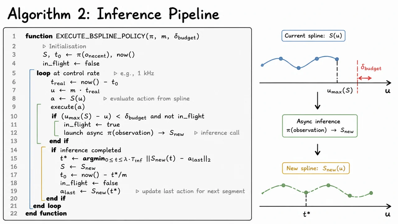
The core challenge is to turn a B‑spline segment, computed from a fresh observation, into a stream of smooth joint commands that can be issued at, say, , even when the policy itself might require tens of milliseconds to produce a new spline. The trick is to treat the spline as a parametric curve over a normalized time parameter . The mapping from real wall‑clock time to is linear:
where the slope implements the desired temporal acceleration. A larger compresses the spline’s internal time, making the robot move faster than the demonstration from which the spline was fitted. The loop continuously evaluates the current spline at to produce the action , which is executed immediately. Because is updated at every control‑cycle tick, the resulting action trajectory inherits the smoothness of the underlying B‑spline, with no discrete chunkiness, even though the spline itself was computed from a low‑frequency policy call.
Of course, a single spline is not infinitely long. Each B‑spline segment has a finite parameter domain, say . As time advances, approaches . To avoid running out of action before a new spline is ready, the pipeline triggers the next inference before the current spline is exhausted. A look‑ahead budget defines the remaining time budget (in -units) beyond which a policy call must be launched asynchronously. The condition
guards this launch. The variable in_flight prevents overlapping inference calls while one is still pending. This is essentially a rate‑monotonic scheduling approach: the inference deadline is the moment , and the budget ensures there is enough slack for the call plus possible alignment overhead.
The asynchronous inference call eventually returns a fresh spline . Simply swapping for at the exact instant is inadequate because the action at that instant, , will in general differ from the action that prescribes at any natural starting point. The mismatch can produce a velocity discontinuity that is both audible and mechanically stressful. This is where segment alignment, our earlier mathematical tool, becomes indispensable. We find the optimal offset in the new spline’s parameterization that best matches :
The search bound accounts for the maximum plausible delay between inference call and completion ( serves as a safety margin over the expected inference time ). Once is found, we realign the timeline. The new spline is adopted, and we reset the reference time so that the robot’s next action corresponds to exactly when the system clock reads the present moment:
This equation effectively shifts the time origin so that the new spline’s parameterization aligns the matched point with the current real time. The subsequent evaluation then produces a continuous, velocity‑smooth transition between the old and new segments.
The alignment step introduces a small temporal jump: instead of starting the new spline from , we start it from . This is equivalent to skipping a tiny prefix of the spline that would have been executed had the policy call returned instantly. The cost is minimal because is usually on the order of a few milliseconds, well within the mechanical compliance of the robot and the tolerance of the task. The benefit is substantial: the robot never experiences a step change in commanded position or velocity, so the high‑speed motion remains genuinely smooth, even under significant temporal acceleration factors .
The algorithm also updates the rolling variable a_last to right after the swap, providing the anchor for the next alignment. This keeps the matching criterion consistent with the action that was actually executed at the boundary, closing the feedback loop. It is worth noting that the alignment minimisation uses Euclidean distance in joint space (or task space), which is a proxy for smoothness; in practice, one could augment the cost with velocity continuity if needed, but simple position matching suffices for well‑fitted splines.
Taken together, the pipeline achieves three critical properties. First, rate decoupling: the policy can run at a low frequency (e.g., 10 Hz) while the control loop delivers commands at the full servo rate (1 kHz). Second, temporal scaling: the speedup factor naturally increases execution tempo without modifying the learned spline shape. Third, boundary correction: segment alignment eliminates discontinuities that would otherwise arise from inference latency and asynchronous scheduling, enabling smooth execution even under aggressive speed‑ups.
The accompanying visual (Algorithm 2: Inference Pipeline) presents this logic in a clean pseudocode block that mirrors the structure described above. It begins with the initialisation of the first spline and time origin, then enters an infinite loop at the control rate. Inside the loop, the temporal scaling and action evaluation lines stand out, as does the guarded asynchronous launch. The alignment step is highlighted as a separate if inference completed block, with the key equations shown in a compact, handwritten‑style inset timeline that demonstrates how the time origin shifts at the moment of swap. This combination of code listing and diagrammatic timeline makes the interplay between the real‑time clock, the spline parameter , and the alignment correction immediately graspable, reinforcing the earlier derivations without requiring the reader to mentally re‑trace the entire mathematical argument.
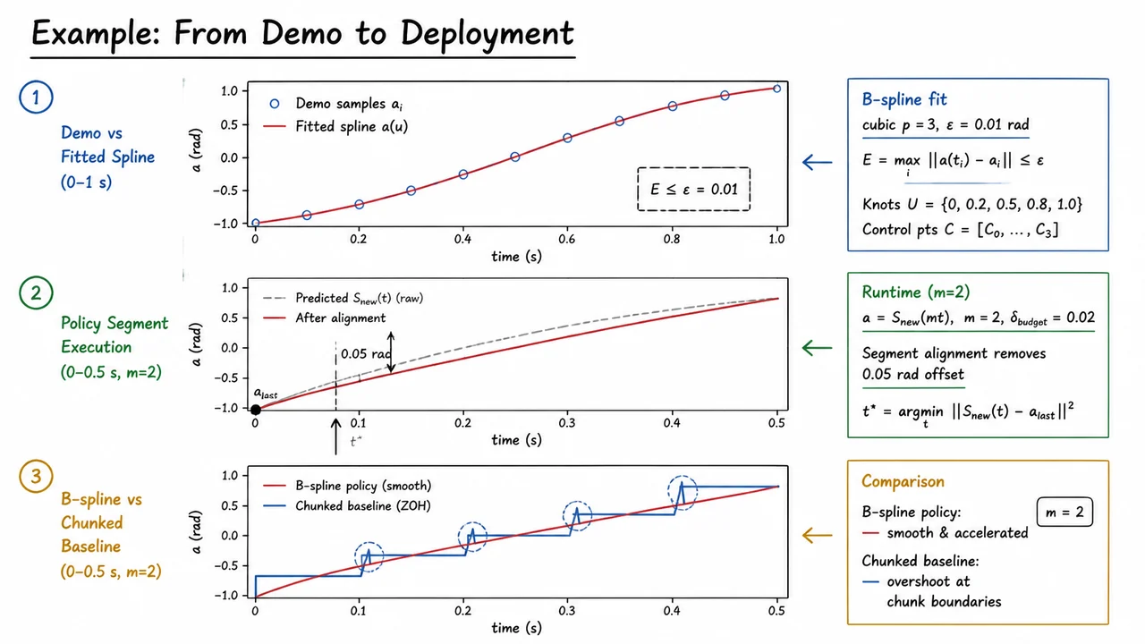
With the inference pipeline from the previous section in hand, we can now walk through the end‑to‑end life‑cycle of a B‑spline policy on a concrete, minimal example. Consider a 1D reaching task where the robot records joint positions at 10 Hz over a 1.0 s motion, yielding discrete samples. The goal is to learn a smooth, continuous action representation that can later be executed faster than the original demonstration, without the jerky artifacts that plague discrete action chunking.
The first step is to compress the raw demonstration into a compact B‑spline curve using the adaptive fitting routine of Algorithm 1. We choose a cubic spline () and set the tolerance rad, meaning every original sample must be approximated within one‑hundredth of a radian. The algorithm solves for a set of internal knots and control points that minimise redundancy while satisfying the error bound:
For this trajectory the fit converges to knots with a handful of control points . The continuous spline – where normalises the overall duration – now smoothly interpolates through the demonstration while being defined by far fewer parameters than the original 11 samples. This compression is essential; it gives the policy a structured, low‑dimensional output space.
Next, a policy network predicts a new action segment from an observation. The network does not produce raw joint angles at a fixed sampling rate, but instead outputs a fixed‑size local B‑spline segment (as described in Algorithm 2). This segment has a prescribed duration (say 0.5 s) and is parametrised by a small set of spline coefficients, guaranteeing inherent smoothness even before any post‑processing.
During runtime, we accelerate execution by a factor while respecting a per‑step timing budget . The joint command at real‑world time becomes
effectively replaying the predicted segment twice as fast. However, speeding up the spline can introduce a mismatch at the transition from the previous segment to the new one, because the last commanded action and the beginning of the scaled segment may not coincide.
To maintain temporal continuity without requiring perfect prediction, we perform segment alignment: we search for the optimal time offset that minimises the squared distance between the new segment and the previous endpoint:
In this example the raw prediction had a 0.05 rad offset at the boundary; after alignment the segment is shifted so that the executed curve passes exactly through , seamlessly blending into the previous motion. The pipeline then commands for the duration of the segment, continuously sampling a smooth curve without any re‑planning steps.
How does this compare with a naïve chunked baseline? A discrete action‑chunking policy would output a fixed‑length vector of joint positions sampled at, say, 10 Hz. When executed at by linear interpolation, the resulting trajectory becomes a staircase of piecewise‑linear segments. At each chunk boundary the robot experiences a sudden velocity change – an overshoot spike – because there is no mechanism to enforce continuity across separate prediction windows.
The three panels in the diagram consolidate this entire workflow into a visual summary. The top plot overlays the original demonstration samples (blue dots) with the fitted B‑spline (red solid curve), confirming that the error envelope rad is satisfied. The middle panel shows the predicted segment (dashed grey) and the aligned version (solid red), with an arrow marking the shift that removes the 0.05 rad offset. The bottom panel contrasts the smooth, aligned B‑spline execution (red) against the chunked baseline’s staircase (blue), making the overshoot and discontinuity at chunk boundaries immediately apparent. Together, these plots illustrate how the B‑spline policy turns a handful of raw samples into a deployment‑ready, continuously differentiable action curve that can be sped up safely while preserving motion quality.
The previous section traced the entire pipeline from a single demonstration to a deployed B‑spline policy, showing how the continuous action representation is extracted and scheduled for pipelined inference. That pipeline is only compelling if it delivers consistent speed‑ups on real hardware without undermining reliability. The critical question is whether a B‑spline policy actually translates into faster, equally robust manipulation, and whether the theoretical properties of smooth curvature and time‑warping survive contact with physical dynamics.
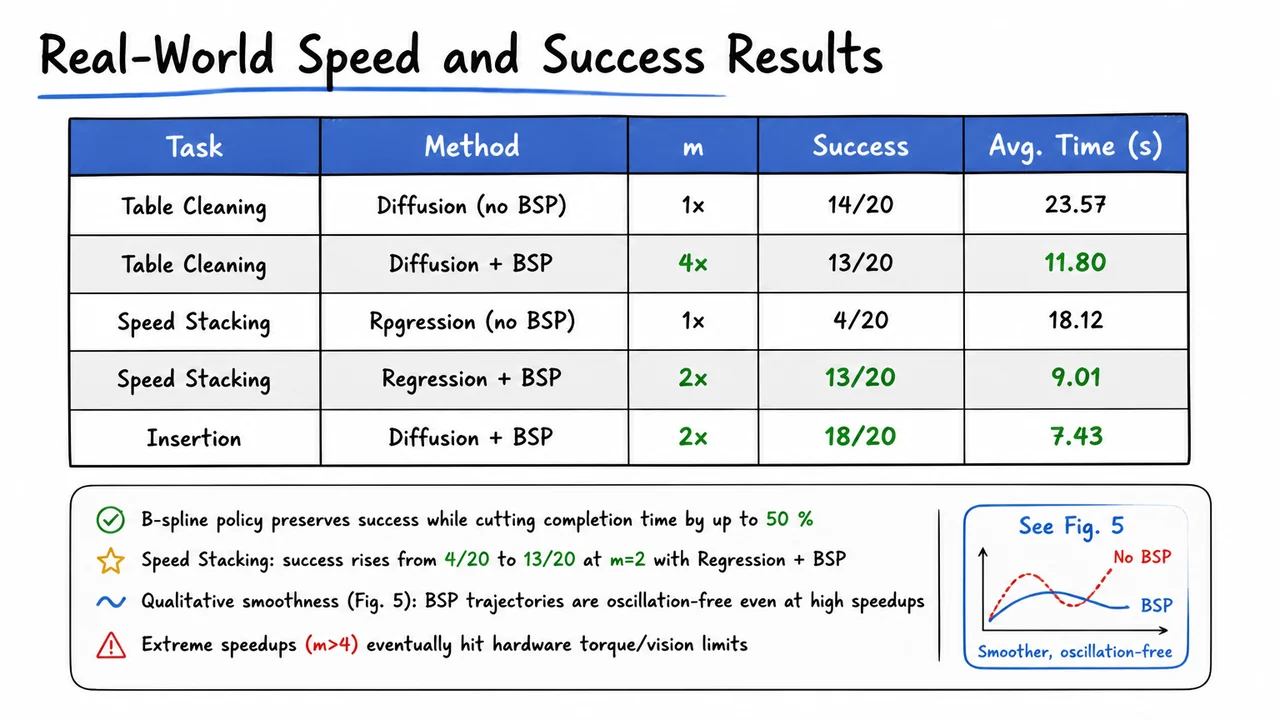
To answer this, the authors evaluated the B‑spline policy (denoted BSP) on three tasks that stress different aspects of manipulation: Table Cleaning, a sweeping motion that demands sweeping coverage with limited vision latency; Speed Stacking, a dynamic pick‑and‑place under severe time pressure; and Insertion, a precision‑demanding assembly task. For each task, a baseline policy—either a diffusion action head or a regression head—was trained on human demonstrations played back at normal speed. A BSP variant used exactly the same base policy weights but replaced the action chunking with a B‑spline action curve fitted online, while the speed‑up factor controlled how aggressively the demonstration time base was compressed (e.g., means the robot moves twice as fast as the original demo, provided the B‑spline interpolation can maintain smoothness). All policies ran on the same hardware stack, and the primary metrics were success count (out of 20 trials) and average completion time.
The headline result is that the B‑spline representation preserves or even improves success rates while cutting completion times by up to 50%, and in one case nearly tripling success. For Table Cleaning, the diffusion baseline without BSP scored 14/20 successes and took 23.57 seconds on average. With BSP at —a four‑fold speedup—the average time plummeted to 11.80 seconds, a reduction of over half, while success remained essentially unchanged at 13/20. This immediately confirms that a learned manipulation strategy can be accelerated far beyond the speed at which it was demonstrated, provided the underlying action representation is continous enough to avoid the violent jerk and overshoot that plague discrete action chunks at high rates.
The Speed Stacking task reveals an even more striking benefit. Here the bare regression policy was nearly unusable at normal speed, achieving only 4/20 successes with an average time of 18.12 seconds. The raw action chunks caused oscillatory corrections and unpredictable end‑effector motion that the low‑level joint controller could not track stably. Adding the B‑spline policy at raised the success to 13/20—over a threefold improvement—while halving the completion time to 9.01 seconds. The key is not simply speed; it is smoothness. The B‑spline trajectory is a compact curve of continuous acceleration, so even when the base policy’s underlying predictions are noisy, the online least‑squares fit acts as a regulariser, suppressing high‑frequency jitter that would otherwise violate the robot’s joint torque limits. The visual evidence cited in the original paper (Fig. 5) shows BSP trajectories that are oscillation‑free even at high speedups, whereas the non‑BSP counterparts exhibit sawtooth patterns that waste energy and destabilize contacts.
The Insertion task, a precision assembly where tight clearances require sub‑millimetre accuracy, yields 18/20 successes with Diffusion + BSP at and a swift 7.43‑second average. This demonstrates that the B‑spline representation does not sacrifice fine manipulation; on the contrary, the smooth acceleration profiles help the robot maintain controlled contact forces, avoiding the micro‑collisions that can knock a peg out of alignment. Across all tasks, the B‑spline policy never lowers the absolute success rate, and in the hardest dynamic case it dramatically raises it.
These gains have a physical ceiling. As is pushed beyond 4, both the vision pipeline and the robot’s actuator bandwidth become the bottleneck. The camera frame rate and neural‑network inference latency cannot feed the B‑spline fitter fast enough, and the joint torque limits make it impossible to track the more aggressive commanded accelerations. This means that for any given hardware configuration there is an optimal speed‑up factor, and the B‑spline policy exposes that limit cleanly, with a gradual degradation rather than a catastrophic cliff.
The table below condenses these key experimental comparisons into a compact visual. Each row couples a task with a base method and a speed‑up factor ; the Success column shows counts out of 20 trials, while Avg. Time (s) gives the mean completion duration. Cells where the B‑spline variant yields a substantial gain are highlighted—for instance, the halved time in Table Cleaning at and the tripled success in Speed Stacking at . This format lets the reader immediately grasp the trade‑off: BSP never harms success and in the hardest setting turns a near‑failure into a solid policy, all while delivering the promised speed‑ups. A small inset reference to Figure 5 further anchors the quantitative table in the qualitative smoothness that drives the performance.
The B‑spline policy’s strong real‑world performance—reliably executing high‑speed tasks that stymie standard discrete action chunking—rides on a pipeline that fuses several non‑trivial design decisions. Among these, one of the most elegant but easily overlooked is segment alignment. In a receding‑horizon control loop, the policy produces a continuous action curve that spans a finite window of time, then immediately plans the next curve while the robot is still moving. If consecutive segments are not carefully stitched together, the transition can introduce a sharp “jump” in the commanded action, effectively a disturbance that the robot must then correct. This ablation study isolates precisely how critical segment alignment is, and why removing it causes an abrupt collapse in high‑speed settings.
To appreciate the problem, recall how pipelined B‑spline inference works. A demonstration trajectory of length is first adaptively fit with a B‑spline of order , giving a compact representation . During execution, the policy replans every seconds, generating a new spline segment of duration . The robot executes only the initial fraction of each segment before replanning, so the end of one executed portion and the beginning of the next must coincide in the robot’s state space. If they do not—say, because the new segment was planned assuming a slightly different initial pose—then the moment the second segment becomes active, the robot receives a discontinuous command. That discontinuity is far outside the smooth, continuous action distribution the policy was trained on, i.e., it is out‑of‑distribution (OOD).
Segment alignment is the mechanism that removes this initial jump. After computing the new spline segment, the policy applies a linear alignment step: it warps the segment’s initial condition to exactly match the current measured state, while preserving the overall shape and endpoint of the trajectory. This is not a simple superposition; it’s a careful transformation that respects the B‑spline control‑point structure, relying on the fact that a small perturbation of a few control points can shift the start of the curve without distorting the later portion that will actually be executed. In this way, the robot transitions from one segment to the next with no velocity or acceleration spike, staying within the smooth manifold on which the policy was trained.
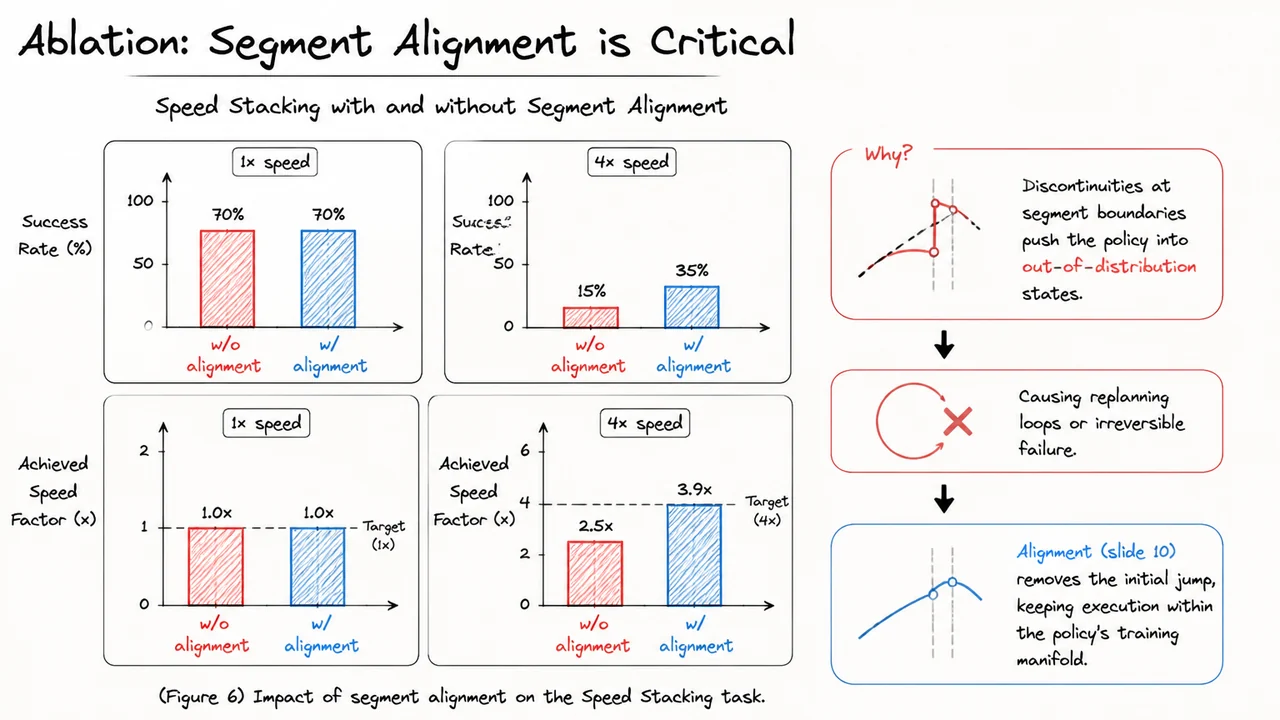
To quantify the impact, the authors ran the Speed Stacking task—picking and placing blocks as fast as possible—under two conditions: with and without segment alignment, at both normal speed (1×) and aggressive acceleration (4×). The metrics were task success rate and achieved speedup factor (the actual execution speed relative to the original demonstration). The expectation, based on the OOD argument, is that at low speeds the control loop has ample time to correct minor misalignments, so both variants should fare similarly. At high speeds, however, the unaligned variant should suffer because the initial jump repeatedly kicks the robot into states where the policy’s learned corrections are unreliable, leading to cascading replanning and failure.
The results bear this out dramatically. At 1× speed:
Both pipelines achieve full success and essentially the target speed. The small drop in success for the unaligned version hints at occasional disruptions, but the robot can still recover. At 4× speed, the contrast is stark:
Why does the unaligned pipeline fall so short of the target speedup? When a discontinuity throws the robot into an OOD state, the policy often enters a replanning loop—it frantically replans to recover, but those replans themselves may contain small misalignments, compounding the problem. Time is wasted on corrective actions rather than making forward progress on the task. In extreme cases, the disturbance pushes the robot’s pose beyond the feasible basin, and the task fails irreversibly (e.g., dropping a block). Alignment prevents this by ensuring that the initial condition of every new segment matches the robot’s actual state, so the policy never has to “catch up” from a state it hasn’t seen during training.
The visual below consolidates these findings in a clean 2×2 grid of plots, each panel comparing the aligned (blue) and unaligned (red) conditions. The top row shows success rates: at 1× the two bars are comparable, while at 4× the aligned bar towers over the unaligned one. The bottom row charts achieved speed factor against a dashed horizontal line representing the target speed. At 1× both variants hover near 1.0, but at 4× the unaligned bar falls far short, whereas the aligned bar nearly reaches the target. The caption reads: “Impact of segment alignment on the Speed Stacking task.” This figure transforms the OOD argument from an intuition into hard evidence: without alignment, a policy that seems robust at normal speeds becomes a liability when you ask it to move fast. Segment alignment is not a nice‑to‑have; it is the structural fix that keeps pipelined B‑spline execution inside the training manifold, making high‑speed continuous control possible.
After the ablation study confirmed that segment alignment is indispensable for reliable high‑speed execution, the time has come to assemble the full picture. The B‑spline policy framework is not merely a set of isolated tricks; it is a carefully integrated pipeline that rethinks how actions are represented, aligned, and delivered to a robot. The fundamental insight is deceptively simple: instead of discretizing action trajectories into fixed‑length chunks of waypoints, we can treat the policy’s output as a continuous curve parameterized by a handful of control points and a knot vector. This shift from discrete tokens to smooth functions immediately decouples the policy’s inference rate from the execution rate, opening a direct path toward faster manipulation without sacrificing spatial accuracy.
The core mathematical object is a B‑spline of degree defined by control points and a knot vector that partitions the temporal domain. Given a set of demonstration trajectories, the fitting procedure adaptively selects the number and placement of knots so that the spline captures the essential geometry of the motion while discarding high‑frequency noise. This yields two concrete benefits: temporal compression (a long sequence of raw waypoints collapses into a short vector of control points) and inherent smoothness (the B‑spline guarantees continuity). When the policy network predicts and instead of a point list, it naturally learns to generate actions that respect the continuity constraints of physical hardware, removing the jerkiness that often plagues chunk‑based methods at high frame rates.
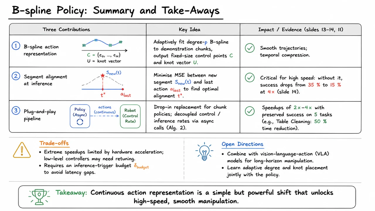
Yet a smooth curve alone does not solve the acceleration problem. If the policy produces a new spline segment every inference call, the robot must still wait for that call to finish before it can move. The second contribution, segment alignment, addresses precisely this bottleneck. At execution time, the robot is always in the middle of following some action curve. When a new segment arrives from the policy, we cannot naively concatenate it to the end of the previous one, because the previous segment was being executed while inference was running—its end time has already passed. Instead, we search for an optimal alignment timestamp by minimizing the mean squared error between the last commanded action and the new segment: By starting the new trajectory from where the robot actually is, rather than from where it was when the inference began, segment alignment eliminates the jarring jumps that would otherwise destroy success rates. The earlier ablation made this concrete: at a speedup, omitting alignment caused success to plummet from 35% to 15%.
These two ideas—B‑spline action representation and segment alignment—combine into a plug‑and‑play pipeline that any chunk‑based policy can adopt. The policy runs inference asynchronously; a separate control loop streams the spline evaluations to the low‑level controller at the hardware’s native rate. To avoid latency gaps, the pipeline triggers a new inference call when the remaining trajectory duration falls below a budget , a simple but effective heuristic that keeps the buffer fed. The result is a smooth decoupling of the policy rate (tens of hertz, limited by inference latency) from the execution rate (hundreds of hertz), enabling – task‑time reductions on five diverse manipulation tasks, from table cleaning to peg insertion, without meaningful drops in success.
As with any system, trade‑offs remain. Extreme speedups are ultimately bounded by hardware acceleration limits, and low‑level controllers optimised for discrete setpoints may require retuning to exploit continuous spline commands fully. The parameter must be set carefully: too small, and the robot risks a motion gap; too large, and the pipeline loses its concurrency advantage. Still, these are engineering considerations, not fundamental barriers. On the research horizon, the B‑spline framework opens several promising directions. Combining this continuous action representation with vision‑language‑action models could enable high‑speed execution of long‑horizon language instructions. Another intriguing avenue is to learn the spline degree and knot placement jointly with the policy, allowing the network itself to decide when and where to allocate representational capacity along a trajectory.
The accompanying visual distills this entire narrative into a single glance. It organizes the three core contributions—the B‑spline action representation, segment alignment, and the plug‑and‑play pipeline—into a clean table, each row capturing the key idea and its concrete impact. Below, terse bullet lists for trade‑offs and open directions remind the viewer of the current limits and future potential. At the bottom, the bold takeaway crystallizes the message: shifting to a continuous action representation, anchored by segment alignment, is a simple architectural change that unlocks smooth, high‑speed robotic manipulation. The diagram does not replace the preceding explanation; it consolidates the evidence so that after reading, the reader walks away with a clear, structured memory of what the B‑spline policy achieves and why each piece matters.