Imagine an LLM solving a math problem. It samples a full reasoning trace, you run a verifier, and the verifier returns a number: perhaps 0 for a correct answer and 1 for an incorrect one, or a richer score measuring how far the solution is from what you want. Once you have that score, the usual modern instinct is to reach for reinforcement learning. Treat the score as a reward, sample trajectories, and update the model so better trajectories become more likely.
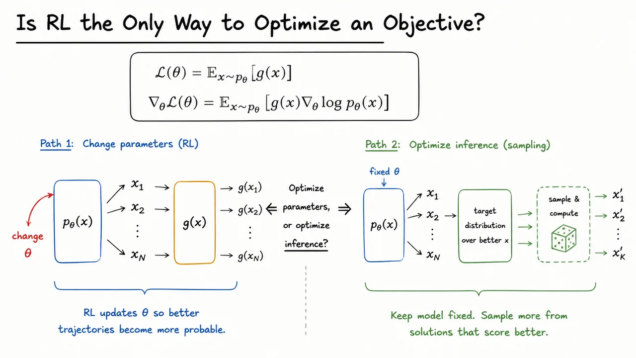
Write the model's distribution over complete solutions as , and let be an objective that we want to minimize. Then the quantity we care about is
REINFORCE gives a way to change the model parameters using only sampled trajectories and their objective values:
The mechanism is simple. A trajectory receives an objective value . The factor tells us how changing the parameters would change the log-probability of that trajectory. Multiplying the two gives a direction for reshaping the model distribution. Repeating this across many samples moves probability mass toward trajectories with better objective values.
That is one way to exploit an evaluable objective, but notice what RL is actually doing: it spends computation modifying . The final product of training is a new distribution from which good trajectories are easier to sample later.
There is another place we could spend the computation. Suppose we leave the base model fixed. Instead of changing its parameters, we could define a new target distribution that puts more probability on better solutions and then use a sampling algorithm to draw from that target. The intelligence would live in the inference procedure rather than in a parameter update.
This changes the design question. Rather than immediately asking, "How do we optimize the policy?", we can first ask, "What distribution over solutions would we like to sample from if computation were not a problem?" Once that distribution is explicit, reinforcement learning becomes one possible route to it rather than the only route.
Suppose there are a million possible reasoning traces. Asking for the single minimizer of is equivalent to solving the original search problem directly. That is often exactly the hard part.
A softer question is easier to work with: can we define a distribution that prefers better solutions without insisting that all probability mass collapse onto the best one immediately?
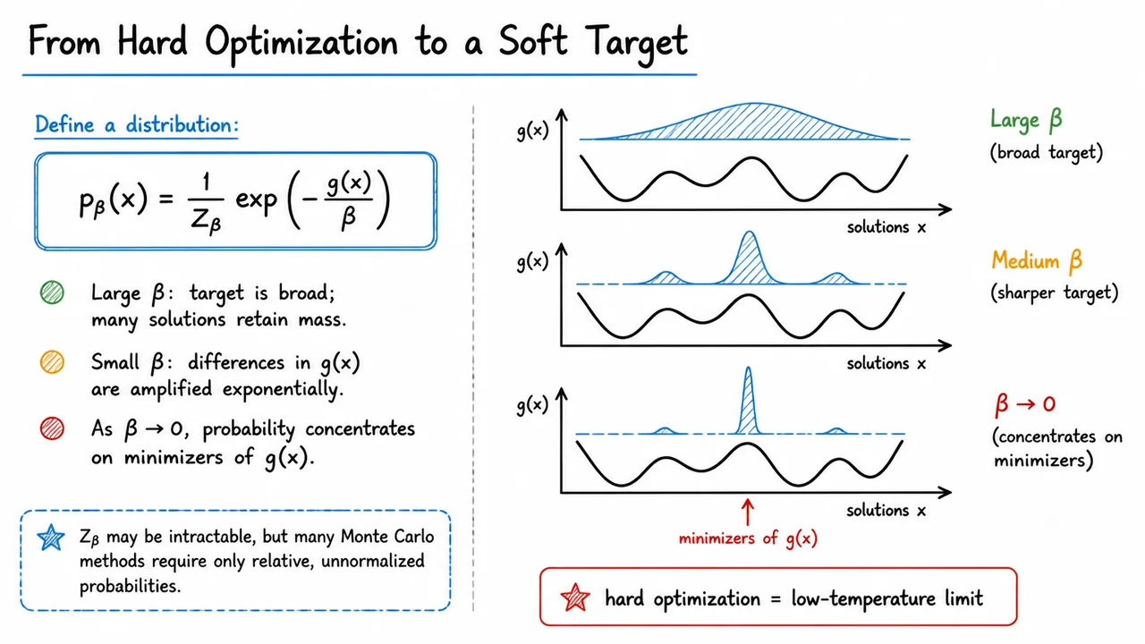
One natural choice is
This is an energy-based distribution. The objective plays the role of energy: lower objective means larger probability. The exponential matters because differences in objective become multiplicative differences in probability. If one candidate has objective 1 lower than another, their relative probability differs by a factor of .
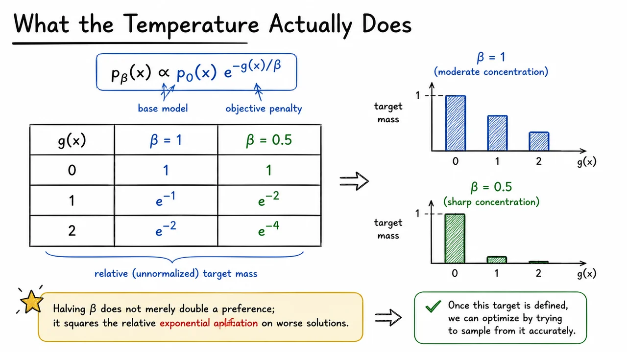
The parameter controls how forgiving the distribution is. With a large , the exponent changes slowly, so mediocre and excellent solutions can both retain substantial probability. With a small , even modest objective differences become decisive. As , the distribution concentrates more and more tightly on minimizers of . Hard optimization therefore appears as a limiting case of a softer sampling problem.
The constant makes all probabilities sum to one. In a large combinatorial space, computing it can be hopeless because it requires aggregating over essentially every possible . Fortunately, this does not kill the idea. Many Monte Carlo methods need only ratios of probabilities or unnormalized weights. In those calculations, the same appears everywhere and cancels.
So we now have a precise target distribution. The remaining simplification is unrealistic, though: this form treats the solution space as if every candidate were equally plausible before looking at . A language model already gives us a strong prior over which sequences look coherent. We should keep that information rather than throw it away.
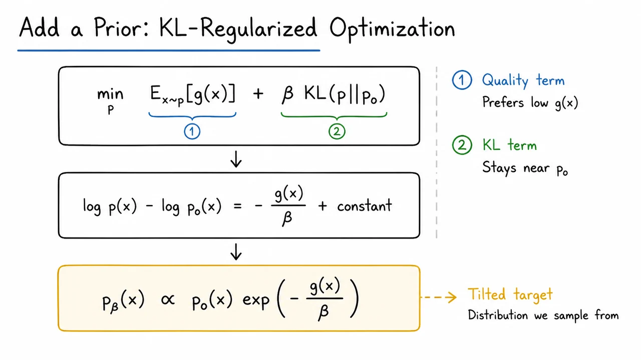
Let denote the base model. We want a new distribution that prefers low-objective solutions while still respecting what the base model already knows about plausible sequences. A clean way to express that trade-off is
The two terms pull in different directions. The expected objective rewards distributions that put mass on good solutions. The KL term penalizes moving too far from . If already assigns almost no probability to a bizarre or syntactically broken reasoning trace, the new distribution must pay a KL cost to place substantial mass there.
The coefficient controls that compromise. A larger makes fidelity to the base model more important. A smaller lets the objective dominate.
Solving this optimization over all distributions gives a simple stationary relation:
Exponentiating both sides gives
This form is useful because it separates two sources of information. The factor says how plausible the solution is under the original model. The exponential factor says how much the external objective should tilt that plausibility. A sequence can be likely under the base model but still be suppressed if it scores poorly; a rare sequence can be promoted if its objective is sufficiently better, but only in proportion to the trade-off set by .
If you have seen KL-regularized RLHF or entropy-regularized control, the structure should look familiar. The point here is narrower: once this distribution has been written down, we can treat it as a sampling target directly. We do not yet need to decide whether we will reach it by changing model parameters, by reweighting samples, by maintaining particles, or by constructing a Markov chain.
A tiny numerical example shows why matters so much. Suppose three candidate solutions are equally likely under , with objective values . Because the base probabilities are equal, their relative target masses come entirely from the exponential factor:
If , the three unnormalized masses are
The best solution is preferred, but the others still have visible probability. Now halve the temperature to . The masses become
The preference did not become merely twice as strong. The exponent doubled, so every relative penalty was amplified exponentially. That is why low temperature can turn a broad distribution into one dominated by a tiny set of trajectories.
This gives two practical interpretations. Statistically, it controls how much probability mass is allowed to remain on suboptimal solutions. Computationally, it controls how hard the sampling problem becomes. A very small produces a target that is attractive from an optimization perspective but may be extremely far from the base model, which makes naive Monte Carlo methods struggle.
Once the target is sharp enough to be useful, we still need a way to draw samples from it. The first method to try is the simplest: sample from an easy distribution and correct the mismatch afterward.
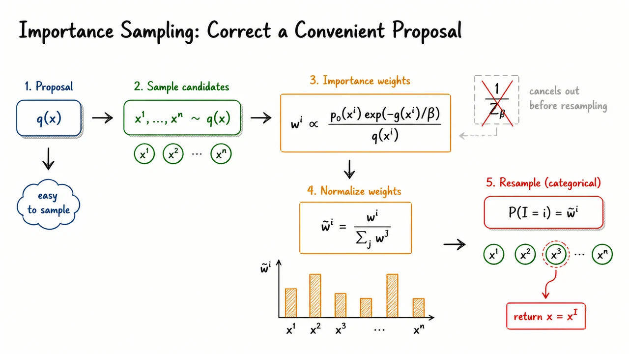
Suppose we cannot sample directly from , but we can easily sample from some proposal distribution . Importance sampling says: generate candidates from , then compensate for the fact that they came from the wrong distribution.
Draw candidates . Each candidate receives an unnormalized weight
The numerator is the target density up to normalization. The denominator corrects for how often the proposal already produces that sample. A trajectory that is common under should not receive extra credit merely because the proposal emits it frequently; the ratio removes that bias.
Normalize the weights,
and then resample an index according to those normalized weights. Returning gives an approximate sample from the target. As the candidate set becomes large and the proposal covers the important regions of the target well, the weighted empirical distribution approaches the target distribution.
The awkward partition function never needs to be evaluated. Every candidate weight would contain the same factor , and that common factor disappears when the weights are normalized.
This is a recurring theme in Monte Carlo methods: knowing relative probability is often enough. The harder question is whether the proposal actually visits the regions where the target places its mass.
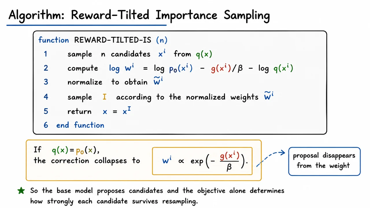
For language models, the most convenient proposal is usually the base model itself. Set . Then the model-probability terms cancel:
The algorithm becomes almost embarrassingly simple. Generate complete candidates with the base model, evaluate for each one, convert those objective values into exponential weights, normalize, and resample.
In a general implementation it is safer to work in log space:
Exponentials can span many orders of magnitude, especially when is small, so direct weight computation can underflow. Subtracting the largest log weight before exponentiating gives the same normalized distribution and is numerically stable.
When , this procedure resembles reward-weighted voting or best-of-, but the objective is different. Best-of- deterministically picks the candidate with the smallest observed . Importance resampling preserves a distribution: a second-best candidate can still be selected with probability determined by its target weight. That matters if the samples will later be used as training data or if we care about approximating a particular distribution rather than returning one winner.
The cancellation also exposes the method's weakness. The base model is doing all of the exploration. Reweighting can promote a good trajectory that was sampled, but it cannot assign weight to a good trajectory that never appeared. For short outputs this may be fine. For long reasoning traces, that limitation becomes severe.
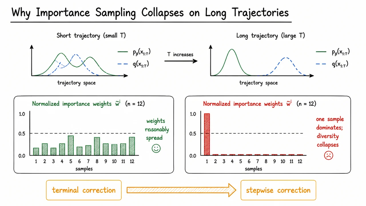
Consider a reasoning trace with hundreds or thousands of token decisions. Even if the proposal is only slightly wrong at each step, those small differences multiply when we look at the probability of the entire sequence. By the end, the proposal distribution over complete trajectories can be very far from the target distribution we actually want.
That distance shows up as weight degeneracy. In a batch of trajectories, perhaps one candidate receives almost all of the normalized mass while the other candidates receive weights close to zero. We technically generated samples, but statistically we may have something much closer to one useful sample.
This becomes worse as the target is sharpened. Smaller increases the reward tilt, so a rare high-quality trajectory can outweigh a large number of ordinary trajectories. If the proposal almost never generates such paths, increasing is the only remedy available to ordinary importance sampling. That can become prohibitively expensive.
The waste is easy to see. Suppose a reasoning trace takes 2,000 tokens and becomes obviously unpromising after token 200. Terminal importance sampling still spends the remaining 1,800 tokens finishing that trajectory before discovering that its final weight is negligible.
A sequential method should do something else: inspect partial trajectories while they are being built, discard weak prefixes early, and redirect computation toward prefixes whose futures still look promising. To do that rigorously, we need a target distribution for a prefix, even though the objective may only be available for complete solutions.
Start from the target over complete trajectories:
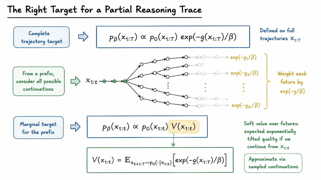
A prefix does not yet have a final objective value. Still, it has a well-defined target probability: add up the target probability of every complete trajectory that begins with that prefix. In other words, marginalize over all possible futures.
Factoring out the probability of the prefix under the base model gives
with
This is a soft value function. It does not ask whether the current prefix looks locally elegant, nor does it ask for the raw expected terminal objective. It asks how much exponentially tilted target mass is reachable if the base model continues from this prefix.
A prefix can therefore look strange in isolation and still deserve high value if it frequently leads to excellent completions. Conversely, a fluent-looking prefix can have low value if most continuations end badly. That future-looking property is exactly what we need to decide which partial trajectories deserve more inference compute.
In practice, the expectation is not available exactly. One can estimate it by sampling continuations from and regressing a value model toward their exponential terminal scores. The quality of this approximation will matter, but once some estimate of is available, the sequential importance correction becomes surprisingly simple.
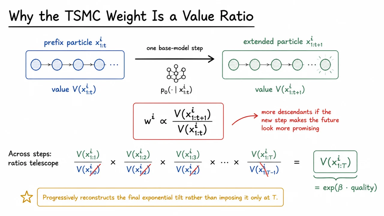
Assume our particles at step are already distributed approximately according to the correct prefix target. To move to step , we extend each prefix using the base model. That proposal introduces the same next-step probability that also appears inside the next prefix target.
When we divide target density by proposal density, those shared base-model factors cancel. What remains is the change in soft value:
This ratio has a useful interpretation. Suppose a prefix had moderate value, then one particular next step makes its future much more promising. Its numerator rises relative to its denominator, so that particle receives a large weight and is likely to be copied during resampling. If the next step destroys most good future continuations, the ratio becomes small and that particle tends to disappear.
The ratio form also explains why the method is sequentially consistent. Multiply the incremental value ratios across many steps and the intermediate terms cancel:
Only the endpoints survive. The final endpoint contains the terminal exponential score, so a sequence of local corrections reconstructs the same global tilt that ordinary importance sampling would have imposed at the end.
That is the advantage of Twisted Sequential Monte Carlo: it does not change the target distribution. It changes when we pay attention to the target, moving the correction earlier so computational effort can be redirected while the trajectory is still being generated.
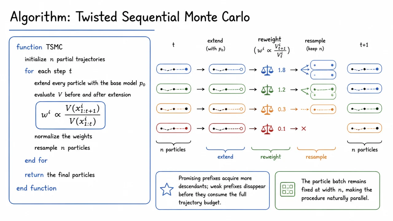
The full TSMC procedure now follows almost mechanically. Maintain partial trajectories. At each step, extend every particle using the base model, evaluate the soft value before and after extension, compute
normalize those weights, and resample back to exactly particles.
Resampling is where computation gets reallocated. Suppose four particles have normalized weights roughly . The next population may contain multiple descendants of the first particle and none of the last one. The algorithm has effectively decided that spending another hundred tokens on the weakest prefix is less useful than exploring several futures from the strongest prefix.
This differs from a search tree in an operationally useful way. TSMC keeps a fixed-width batch. At every generation step there are still sequences to process, even though their ancestry changes. That makes the method well suited to accelerator-friendly batched decoding. There is no need for a dynamically widening tree with irregular numbers of nodes at different depths.
The price is the value function. If is badly estimated, resampling can kill a prefix whose future was actually excellent or duplicate a misleading one. Repeated resampling can also reduce diversity when many particles share the same ancestors. These are the sequential analogues of proposal quality problems in importance sampling.
Still, TSMC solves the specific waste we identified earlier: it does not wait until a complete trajectory is generated before deciding where inference compute should go. A different family of methods takes an even more iterative approach—rather than maintaining many evolving particles, keep a current solution and repeatedly revise it.
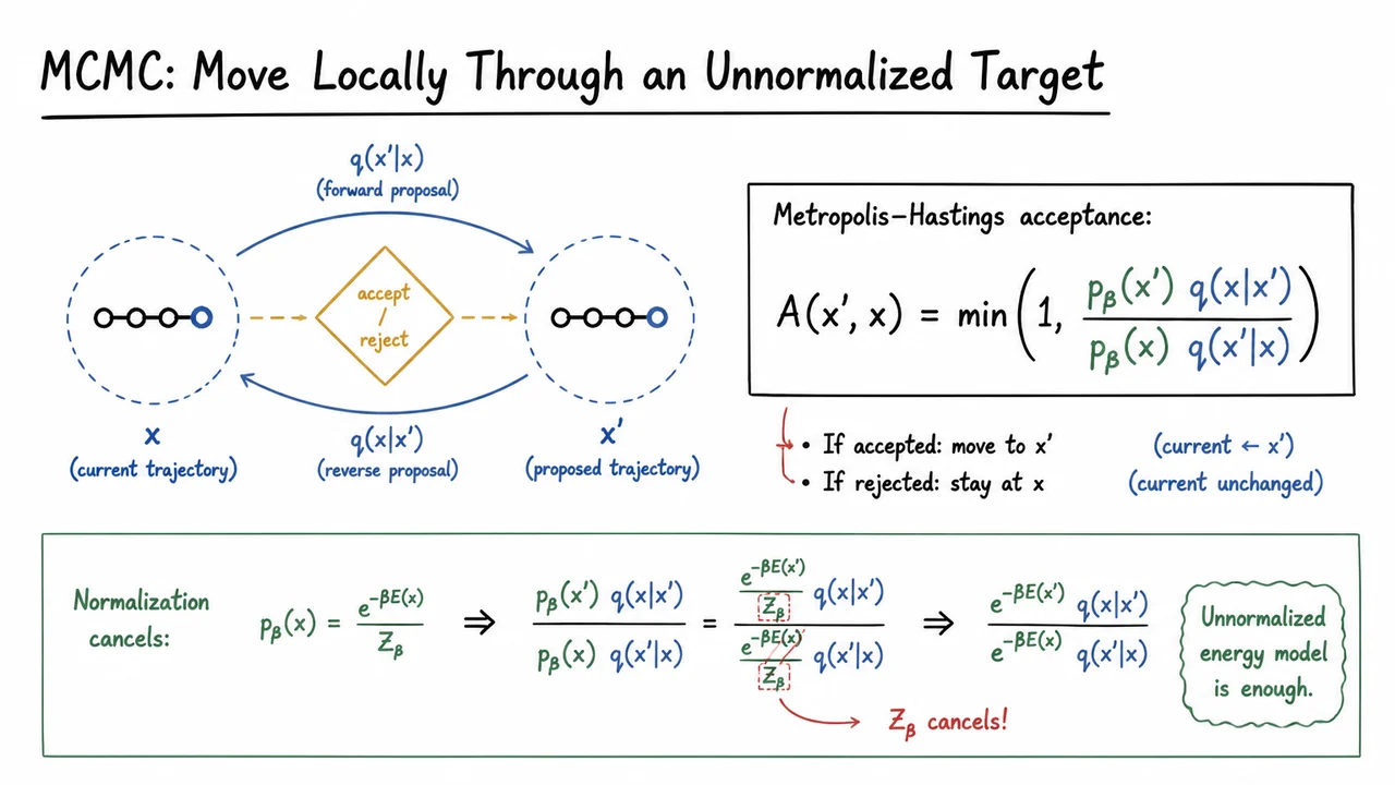
Markov chain Monte Carlo starts from a different computational bargain. Instead of repeatedly generating independent trajectories from scratch, keep one current trajectory and propose a nearby alternative . Then decide whether that proposed move should become the next state of the chain.
Let the proposal mechanism be . Metropolis-Hastings accepts the proposal with probability
If the proposed state is much more probable under the target, acceptance is likely. If it is worse, it can still be accepted sometimes. That randomness matters: a chain that only accepts improvements would behave like a local optimizer and could become trapped around one mode instead of representing the full target distribution.
The proposal terms correct for asymmetric moves. If moving from to is easy under but the reverse move is unlikely, the acceptance ratio accounts for that imbalance. Under the usual conditions, this correction gives the target distribution the right stationary probability flow.
Again, the partition function disappears. Because is needed only through a ratio, the same occurs in numerator and denominator and cancels. We can therefore run MCMC with an energy-based target known only up to proportionality.
The challenge shifts from normalization to proposal design. If proposals make tiny, uninteresting changes, the chain moves slowly through the space. If they make enormous changes, most proposals may be rejected. For language-model trajectories we need a move that is large enough to revise reasoning but structured enough to remain plausible.
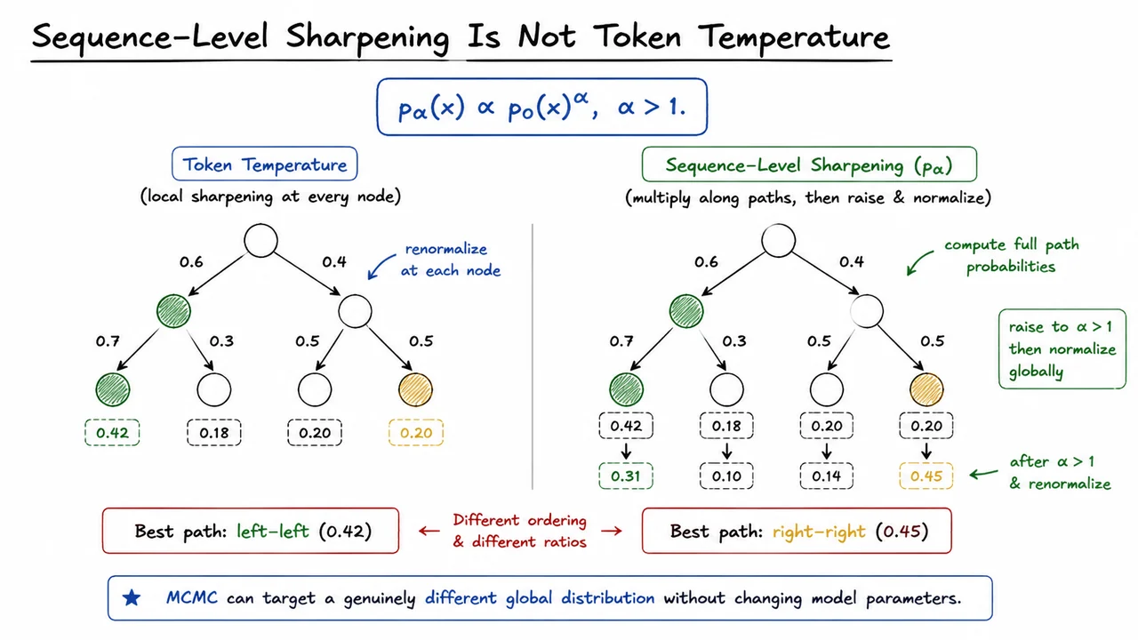
One target studied in this setting does not use an external reward at all. Instead, take the base model's probability of a complete trajectory and sharpen it globally:
If one full reasoning trace is ten times as probable as another under , then with it becomes one hundred times as probable before normalization. The transformation concentrates mass on sequences the model itself already judges relatively likely.
It is tempting to say this is just lower-temperature decoding. It is not. Ordinary temperature sampling modifies each conditional distribution and renormalizes locally at every token. Sequence-level sharpening first considers the probability of the whole trajectory—the product of all those conditionals—and then raises that complete probability to before one global normalization.
Those operations do not generally commute. Local normalization changes how probability is distributed inside every branch of the generation tree. Two paths can therefore receive different relative mass under token-level sharpening than under global sequence-level sharpening, even when the same exponent is used.
That difference matters because is easy to evaluate from the base model but awkward to sample from directly. This is exactly the setting where Metropolis-Hastings is useful: construct plausible edits with the language model, then use accept/reject correction to make the resulting chain target the desired global distribution.
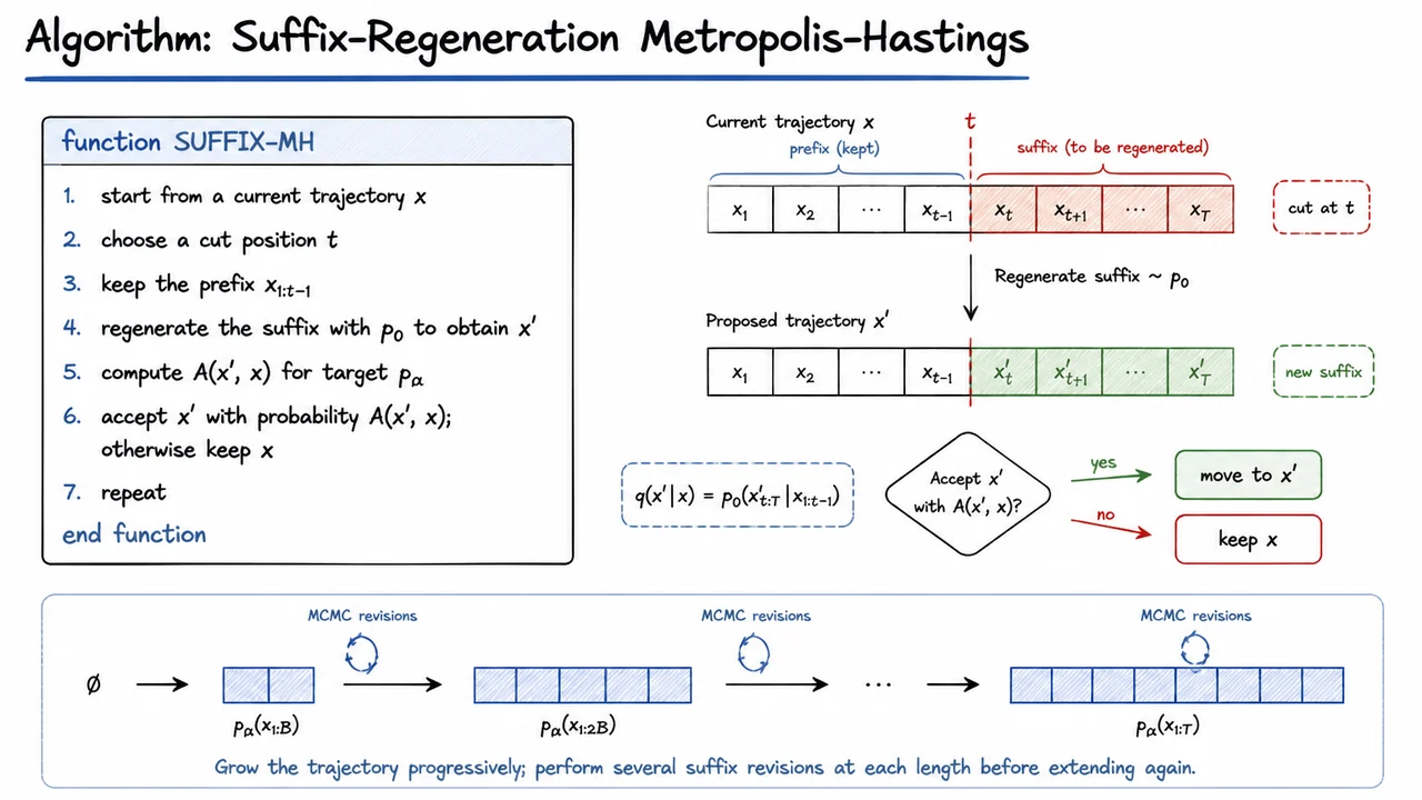
A simple proposal for an autoregressive language model is to reuse part of the current reasoning trace and regenerate the rest. Choose a cut position , keep the prefix fixed, and ask the base model to sample a fresh suffix. The proposal density is therefore
This move is attractive because it is easy to sample and easy to score. The model does the work it already knows how to do: continue from a prefix. The Metropolis-Hastings acceptance rule then decides whether the newly generated suffix moves the chain in the right distributional direction.
Repeated suffix regeneration lets the model revise its own reasoning. A cut near the end makes a small local edit; a cut near the beginning can replace most of the solution. The proposal therefore spans a range of move sizes without requiring a separate learned editor.
Very long sequences still create a mixing problem. Jumping directly into MCMC over a full -step trajectory can leave the chain dependent on a poor initial solution for a long time. A practical remedy is to grow the target progressively:
First sample and refine a short prefix. Extend it by another block of steps, run several suffix-regeneration updates at that length, then extend again. Each stage supplies a reasonable initialization for the next, longer problem.
This begins to look like a bridge between SMC and MCMC. SMC grows trajectories sequentially and reallocates particles; sequential MCMC grows the represented trajectory while performing multiple local refinement moves at each stage. Both spend inference compute correcting a distribution before the final answer is complete.
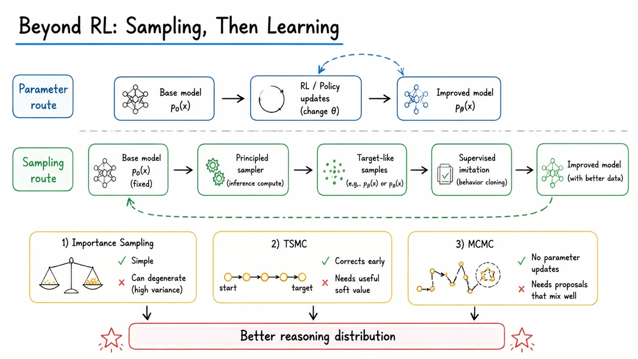
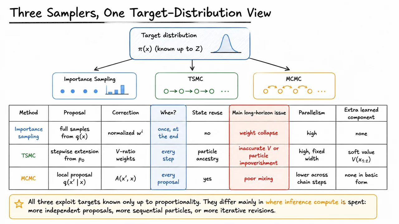
Seen from far enough away, importance sampling, TSMC, and MCMC are solving the same kind of problem: we know a target distribution up to proportionality, direct sampling is hard, and we need to spend inference compute in a way that makes our samples look more like that target.
Importance sampling spends that compute on breadth. Generate many complete candidates independently, score all of them, and correct once at the end. It is simple and embarrassingly parallel, but it fails badly when the proposal and target have little overlap.
TSMC spends compute on a population that evolves through the trajectory. Each particle is extended, reweighted, and resampled repeatedly. It can avoid wasting full rollouts on weak prefixes, and its fixed particle width maps cleanly to batch hardware. Its main extra burden is the soft value , whose errors can misallocate particles.
MCMC spends compute on revision. A state is reused, edited, and either accepted or rejected. This avoids the need to generate every candidate independently, and basic Metropolis-Hastings needs no learned value model. The trade-off is correlation: if proposals are poor, the chain mixes slowly and many updates provide little new information.
So the practical choice is less about which method is universally "better" and more about the geometry of the problem. If complete high-quality trajectories already appear often enough under the proposal, importance sampling may be sufficient. If failures can be detected through predictive prefix values, TSMC can allocate compute earlier. If useful solutions can be reached through local or suffix-level revisions, MCMC offers another route.
The common thread is more important than the taxonomy. In all three cases, we can improve the distribution of reasoning trajectories without first updating the model parameters. That makes sampling itself a serious optimization primitive rather than merely a decoding detail.
Once a sampler can produce trajectories from a distribution we actually want, the boundary between inference and learning becomes less rigid.
RL spends compute updating so that itself assigns more probability to desirable outputs. The samplers above can leave fixed and instead spend inference compute producing samples that approximate or . Both routes try to change the distribution of trajectories we ultimately see; they pay for that change in different places.
That suggests a modular learning loop. First use a principled sampler to generate target-like trajectories. Then train a model with supervised learning to imitate those samples. The expensive sampler acts as a teacher whose behavior is gradually distilled into a cheaper one-shot model. After imitation, the improved model can become a better proposal for the next round of sampling.
This perspective also explains why principled sampling is more attractive than an arbitrary decoding heuristic as a source of training data. A heuristic may return solutions that happen to score well, but it may be difficult to say what distribution its outputs represent. Importance sampling, SMC, and MCMC are designed around explicit targets. Under their assumptions, their samples have a probabilistic interpretation that can be carried into a learning objective.
None of this makes RL obsolete. Policy optimization may be the right tool when changing parameters directly is efficient, when inference-time sampling would be too expensive, or when we want to amortize improved behavior into the model immediately. The broader point is that an evaluable objective creates a design space: update parameters, allocate inference compute, or combine the two.
For long-horizon reasoning, the most promising systems may do exactly that—sample, revise, reweight, learn from the resulting trajectories, and repeat. RL is one way to move probability mass toward better solutions. It is not the only one.