Imitation learning has quietly become one of the most reliable ways to teach robots complex visuomotor skills. By watching a human teleoperator demonstrate a task just a few dozen times, a policy can learn to map raw pixels to joint commands with striking precision. In academic benchmarks, these policies often reach success rates above 90%, and the visual quality of the resulting motion looks remarkably human-like. Yet when the same policy is asked to work outside the carefully timed rhythms of the lab, things can go wrong in ways that have nothing to do with perception or control. The problem is speed: the policy executes at approximately the tempo of the original demonstrator, and that tempo is almost never fast enough for a production task.
The root cause lies not in the learning algorithm but in the data collection process itself. Demonstrations are captured by a human operator using a teleoperation interface—sometimes a VR headset, sometimes a 3D mouse, sometimes a lead-through teach pendant. No matter the tool, the operator suffers from a fundamental sensory and embodiment gap. Humans lack the 3D depth perception of a wrist-mounted camera, cannot feel the fine tactile feedback that a force-torque sensor would provide, and possess a hand morphology that does not match the gripper they are controlling. The result is a pervasive tardiness: even an expert demonstrator moves far more slowly than what the robot’s hardware can physically achieve. Deliberate, cautious movements become baked into the demonstration data, and the imitation-learned policy faithfully reproduces that same unhurried cadence.
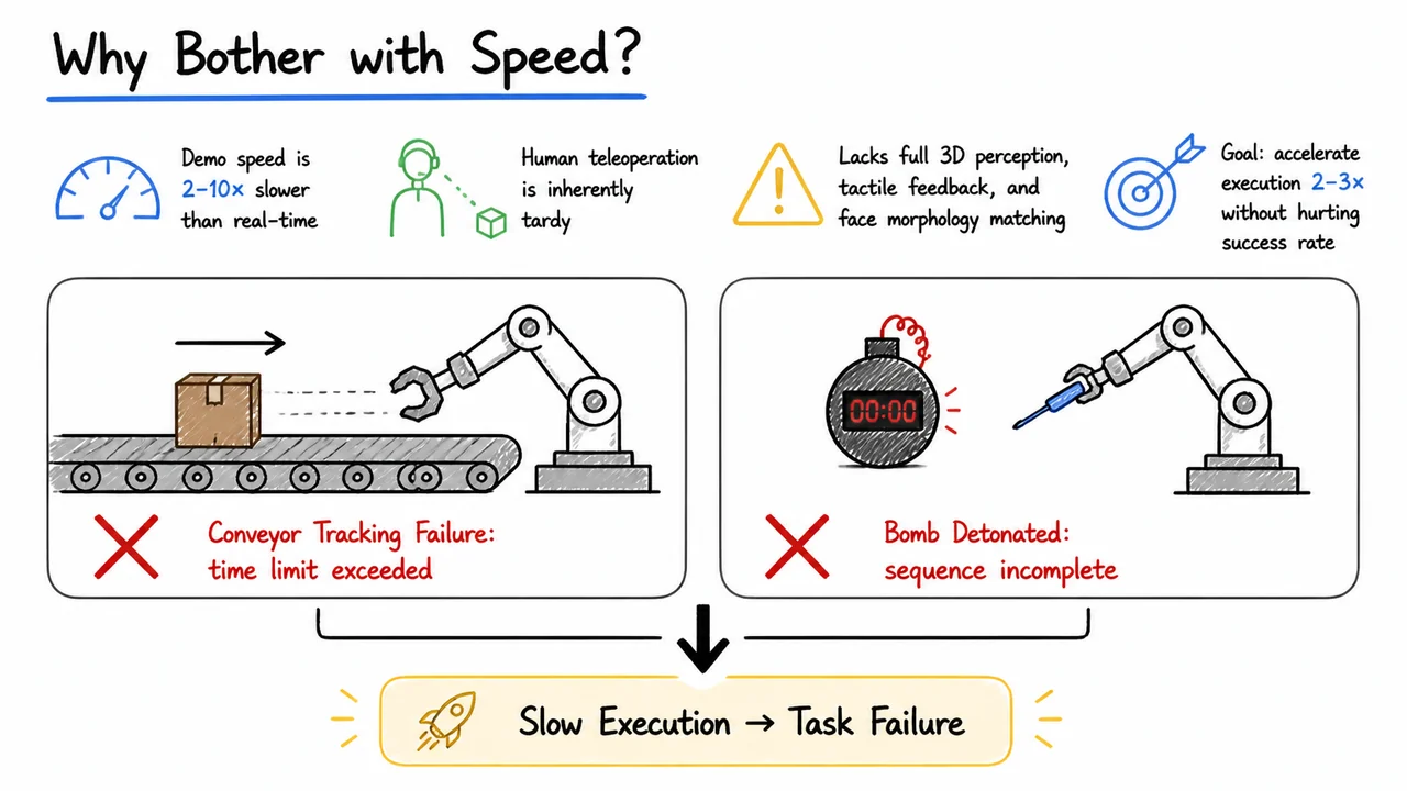
This is not merely a cosmetic flaw. Many real-world tasks have an intrinsic time budget. A classic example is a conveyor belt tracking scenario: a robot must intercept, grasp, and move an object that is continuously sliding along a belt. If the arm’s reach-and-grasp action is even half a second too slow, the object will have moved out of the graspable zone. The policy may still complete the motion flawlessly, but it will close its fingers on empty air—a failure that a human observer would label as “the robot was too slow,” not “the robot did not know where to grasp.” Another telling case is a bomb-defusal toy, a popular benchmarking task where the robot must insert a pin or cut a wire before a visible countdown timer reaches zero. A policy trained from leisurely demonstrations will methodically approach the fuse, but the timer will expire while the gripper is still en route. The robot does not fail because it misunderstands the geometry; it fails because it cannot beat the clock.
These failures expose a subtle but dangerous assumption in imitation learning: the environment will wait for the policy. In static pick-and-place tasks, it often will. But in dynamic, safety-critical, or competitive settings, time is a first-class resource. The conveyor belt and the bomb toy are not edge cases; they are prototypes of a broad class of time-sensitive applications that include surgical assistance, disaster response, and cooperative manufacturing. A policy that succeeds at demonstration speed but cannot accelerate becomes a liability.
The naive solution might be to simply operate the teleoperation faster during data collection. Unfortunately, this rarely works. Pressing the operator to move faster typically degrades the quality of demonstrations, introducing jerky motions, missed grasps, and unsafe collisions—all of which the policy then learns. Moreover, the operator’s inherent sensory latency and lack of direct force feedback set a hard ceiling on how quickly they can safely teleoperate. So we are left with a dilemma: the demonstrations we can collect are slow, but the tasks demand speed.
This is where DemoSpeedup comes in. Its central premise is that we can take a policy trained on slow, high-quality demonstrations and accelerate its execution at test time without sacrificing task success. The target is a speedup of 2–3×, enough to bring a 30‑second demonstration tempo down to the crisp 10–15‑second range required by a conveyor or a countdown timer. Importantly, the acceleration must not merely fast-forward the motion; it must preserve the delicate contact transitions, approach angles, and grasp timing that made the original policy effective. The goal is safe, semantics-preserving acceleration, not reckless fast motion.
Before diving into how DemoSpeedup achieves this, it is helpful to solidify the problem with a concrete mental image. The two failure modes—conveyor belt tracking and bomb timer expiry—represent opposite sides of the same coin: a policy that is competent in space but incompetent in time. The visual that follows captures this duality through a split-panel diagram. On one side, a robot arm reaches toward a box sliding along a conveyor belt, but its gripper lags behind the moving target, marked with a red “X” to signal failure. On the other side, a bomb countdown has already hit 00:00 while the arm is still partway through a defusal maneuver, again marked with a red “X.” A central downward arrow connects them with the label “Slow Execution → Task Failure.” The clean, hand-drawn aesthetic and minimal color palette—red for failure, white background—make the consequences of tardiness unmistakable. This diagram does not present new information; it consolidates the argument into a single glance, reminding us that speed is not a luxury but a requirement for any policy that must interact with the world on the world’s own timeline.
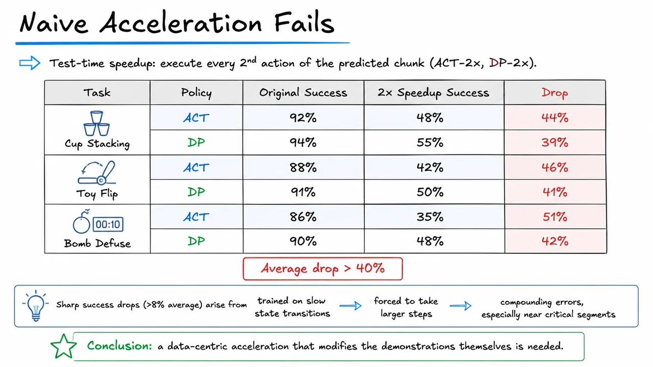
If the promise of speed sounds compelling, the most tempting shortcut is to simply ask a trained policy to move faster at deployment. After all, modern visuomotor policies like ACT (Action Chunking Transformer) and Diffusion Policy (DP) already predict a short sequence of future actions—a chunk of duration —before the next re‑planning step. A natural first experiment is therefore test‑time downsampling: at every control cycle, execute only every second action from the chunk, effectively doubling the robot’s motion speed without changing the trained policy weights. In principle the policy still sees the same visual observations and conditions; only the enacted trajectory is stretched to cover the same spatial extent in fewer time steps.
The appeal of this strategy lies in its simplicity. No retraining, no new data, no extra hyper‑parameters. For ACT‑2× and DP‑2×, one simply drops odd‑indexed actions. A glance at the nominal high success rates of those policies—often above 85% on dexterous tasks—can make it seem as if the learned behavior will gracefully tolerate a mild increase in cadence. Unfortunately, the experimental reality demolishes this hope. Across three fine‑manipulation tasks (cup stacking, toy flipping, bomb defuse), the success rates of both ACT and DP collapse dramatically when naive 2× speedup is applied. The performance drop is not a few percent; it is a catastrophic erosion of reliability, averaging over 40 percentage points. A policy that previously stacked cups 92% of the time now succeeds only 48% of the time. The same pattern repeats with diffusion‑based policies: a 94% base success on cup stacking becomes 55%. This is not a model‑specific fragility; it is a structural failure of the deployment strategy.
The root cause is a subtle but well‑known pathology in imitation learning: distribution shift between the training and testing regimes. During training, the policy learns to generate actions that map a current state to a near‑future sequence under the slow demonstration dynamics. The demonstrations were recorded at a fixed, deliberate pace, often with the human moving smoothly but not hurriedly. Consequently, the policy’s learned mapping implicitly encodes the temporal correlation structure of those slow transitions—how much the end‑effector position, orientation, and object pose change per step. When you suddenly ask the policy to produce actions that span twice the physical displacement in the same amount of prediction time, you are forcing it to operate in a part of the joint state–action space where it has never received supervision. The model’s interpolation and extrapolation abilities are limited; it produces actions that, while plausible in isolation, accumulate small errors that rapidly compound over time.
Compounding errors are especially deadly in contact‑rich manipulation. In cup stacking, a slightly misaligned grasp can cause the cup to slip; in toy flipping, a premature release ruins the flip trajectory; in bomb defuse, a few millimeters of inaccuracy can mean mission failure. These critical moments often require precise, fine‑grained temporal coordination. When the policy is forced to take larger steps, the linear approximations that underlie action‑chunk models break down—the predicted chunk no longer respects the continuity of the physics that the training data implied. Each erroneous action pushes the system into a state the policy has never seen, and from there the predictions become even more erratic. The error compounds geometrically, and within a few timesteps the robot is hopelessly off‑track.
The table in the visual below distills this phenomenon into a crisp, uncomfortable truth. It lists the three tasks, the two policy architectures, the original success rates (serving as a baseline), the success rates after 2× downsampling, and the absolute drop. The numbers are stark, but the presentation also underscores an important lesson: the failure is invariant to the choice of policy family. Both ACT, which uses autoregressive transformers to decode sequential actions, and Diffusion Policy, which refines action chunks via iterative denoising, suffer nearly identical degradation. This cross‑model consensus confirms that the issue is not about representation; it is about the temporal granularity of the demonstrations.
The visual also highlights the “Drop” column with a red accent, making the average drop > 40% impossible to miss. This design choice turns the table into more than a data repository—it becomes a rhetorical device, shouting that naive acceleration is not a viable path. The light blue row banding and crisp typography keep the information legible, while the table title “Test‑time 2× downsampling drastically hurts success” primes the viewer for the diagnosis. By placing this evidence front and center, the slide serves as a pivot point: it closes the door on any lightweight deployment hack and makes the case that only a data‑centric approach—one that modifies the demonstrations themselves—can deliver genuine acceleration without sacrificing task competence. The next sections will build that approach from first principles, starting with the intuition that not all timesteps in a demonstration are equally precise.
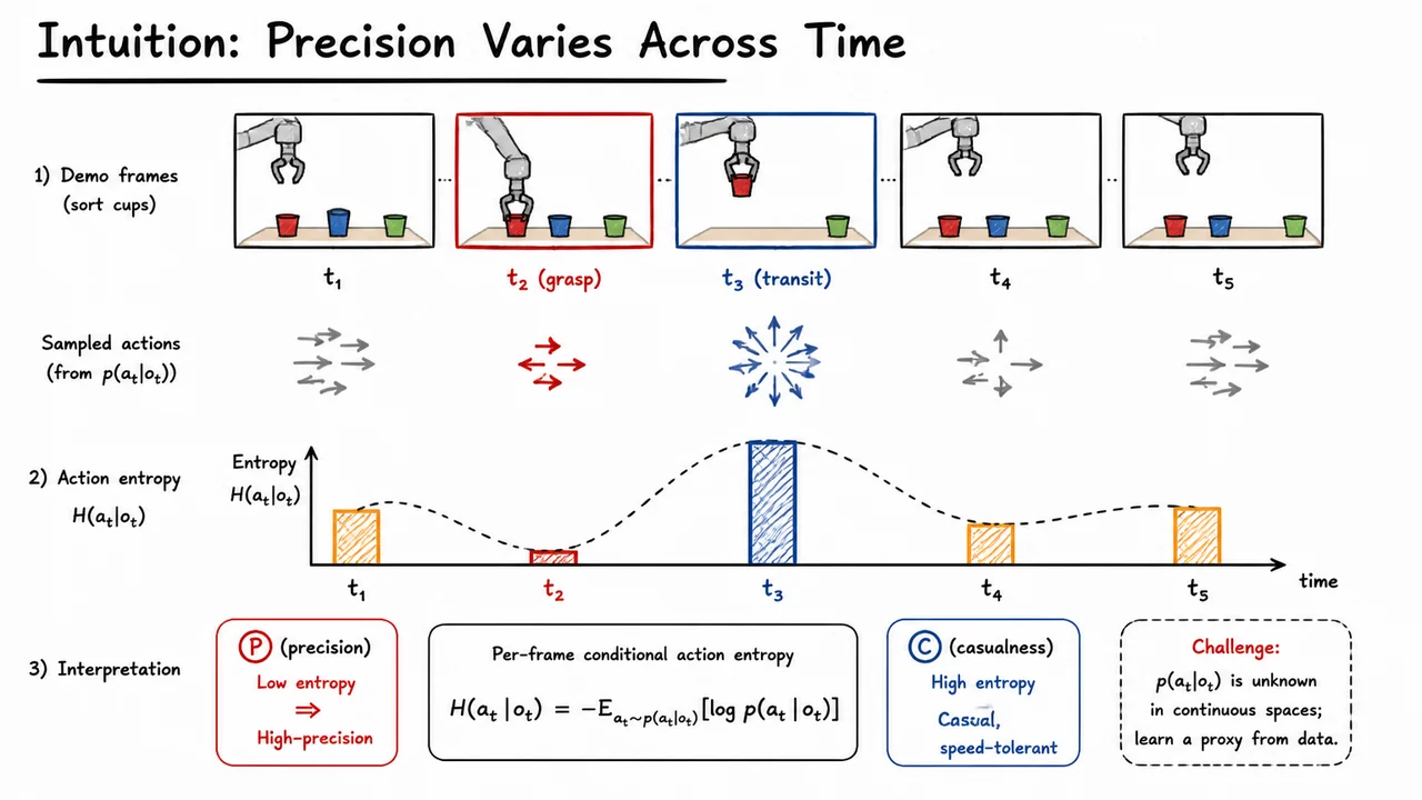
The failure of uniform frame dropping discussed earlier points to an uncomfortable reality: the cost of losing a single RGB–action pair is not constant across a trajectory. Some instants capture moments where the policy must act with near-identical precision to the human teacher or risk catastrophic failure—think of the final approach before a grasp, or a delicate insertion after contact. Others capture long, lazy transits where small perturbations in the chosen joint velocities hardly affect the outcome. Naively removing every second frame destroys both with equal carelessness. The missing insight is that precision varies over time, and any acceleration scheme must respect that variation.
Human teleoperators intuitively adjust their precision. When contact is imminent—when the robot is closing its gripper around a mug—the demonstrator stabilizes their hand, producing a tight, low-variance stream of actions. In free space, the same demonstrator might wave loosely toward the target, yielding high-variance actions that are largely interchangeable. This behavioral regularity suggests a powerful signal: action variability itself reveals how much precision each timestep demands. If we can measure how “spread out” the distribution of plausible actions at a given observation is, we can automatically decide where the trajectory can be safely sped up and where it must remain slow and careful.
The natural mathematical proxy for this variability is the per‑frame conditional action entropy:
Here is the true distribution over actions a skillful policy might output when seeing observation . The entropy quantifies how many “bits of uncertainty” remain about what action to take after seeing the current sensorimotor context. When the distribution is sharply peaked around a single action, the entropy is low: the situation demands precision, and any substitute action would be clearly wrong. When the distribution is broad and many actions are almost equally acceptable, the entropy is high: the situation is casual, and the exact action matters little for task success.
This gives us a clean, unsupervised, task‑agnostic principle:
Crucially, this signal is not something we design by hand for each task; it emerges from the natural variance in human demonstrations. A teleoperator struggling to align a peg produces low‑entropy, highly consistent action streams, while the same operator moving through empty space produces high‑entropy, messy streams. By simply profiling the entropy along the time axis of a demonstrated trajectory, we can flag exactly where the demonstration demands slow, patient imitation and where it can be safely compressed.
There is, of course, a fundamental challenge: in continuous action spaces (e.g., 6‑DOF end‑effector deltas or joint torques), we never observe the true distribution from a single demonstration. A single trajectory gives at most one action sample per observation. We cannot compute the entropy directly. Instead, we must learn a proxy distribution that captures the variability observed across multiple demonstrations of the same skill or, more cleverly, by exploiting the structure of the policy itself. This will be the cornerstone of the DemoSpeedup method, and we will unpack it in the next section.
The diagram that accompanies this section makes the entropy‑precision link tangible. It shows a snapshot of a cup‑sorting trajectory: five evenly spaced video frames, with two moments explicitly highlighted. A grasp frame is framed in red and displays tiny, tightly clustered action arrows beneath it—visual proof of low entropy. A mid‑air transit frame is framed in blue, with arrows fanning out widely to capture the high‑entropy casualness. Below the frame strip, a hand‑drawn time axis plots an entropy curve as a series of vertical bars connected by a dashed arc: the grasp yields a short bar (low entropy), the transit a tall bar (high entropy). A simple legend labels red as “P (precision)” and blue as “C (casualness)”, driving home the central intuition: entropy varies substantially along a trajectory and identifies exactly where speed‑up is permissible. This visual conspectus turns the abstract notion of conditional entropy into an immediately legible design principle, setting the stage for how DemoSpeedup will later segment trajectories into precision and casualness sets to guide informed downsampling.
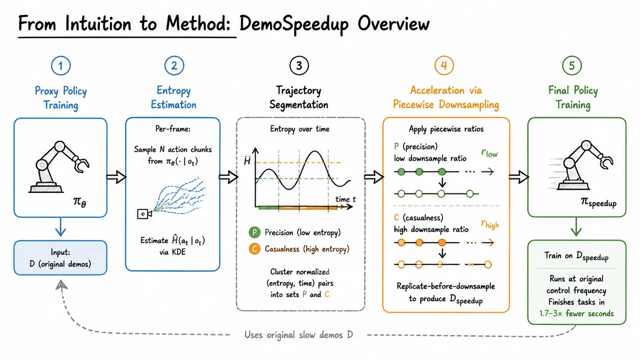
Having established that human demonstrations naturally contain stretches of casualness—intervals where the operator moves slowly, pauses, or generates noisy, unforced actions—the immediate question becomes: how can we systematically identify which moments require careful reproduction and which can be accelerated without harming the task? The DemoSpeedup method answers this by turning the tardiness of the original demonstrations into a measurable signal. Instead of relying on hand‑crafted heuristics or task‑specific timing assumptions, it estimates, for every frame, how uncertain a well‑trained imitation learner would be about the next action. That uncertainty, quantified as per‑frame action entropy, becomes the guidepost for a principled time‑warping procedure. The result is a clean pipeline that automatically distills slow demonstrations into a faster, yet equally successful, control policy.
The first stage builds a proxy policy —a generative action‑chunk model trained exclusively on the original, un‑accelerated dataset . Crucially, this policy is never deployed on a real robot; its sole purpose is to serve as a statistical probe of the demonstration distribution. Because the proxy has been optimized to imitate the slow teleoperated behavior, its conditional distribution captures both the intended action and the demonstrator’s inherent variability. In precision moments, where the demonstrator was focused and consistent, the proxy will concentrate its probability mass tightly around a single action mode. In casualness segments, where the operator meandered, the proxy will reflect a broad, multi‑modal spread of plausible actions. Thus, even though the original trajectories are already recorded, retraining a flexible generative model on them distills the demonstrator’s latent precision structure into a form we can query at every timestep.
To turn that intuition into a quantitative score, the second stage performs entropy estimation. For each observation , the proxy is sampled times to produce a set of candidate action chunks. The per‑step action entropy is then estimated via kernel density estimation (KDE) over those samples. A Gaussian kernel is typically used, and the bandwidth is chosen to balance bias and variance across the range of observed action magnitudes. The outcome is a time‑varying entropy curve that rises in the parts of the task where the demonstrator wavered and falls where the demonstrator was deliberate. This signal is entirely unsupervised—it emerges from the demonstration data itself, without any external labels of precision or urgency.
Because raw entropy values can be noisy and because the goal is to preserve contiguous motion segments, the third stage reframes the entropy curve as a trajectory segmentation problem. Each frame’s normalized entropy and its time index form a point in a 2‑D space, and a density‑based clustering algorithm groups these points into a precision set (low entropy, high action certainty) and a casualness set (high entropy, high variability). Density‑based clustering is a natural fit here: it can discover arbitrarily shaped clusters without pre‑specifying a fixed number of segments, and it naturally filters out noise. The resulting partition often yields several alternating blocks of and along a trajectory, each corresponding to distinct phases—a careful approach, a rapid repositioning, a delicate grasp, and so on.
With the segmentation in hand, the core acceleration step applies piecewise downsampling. During precision blocks the method keeps a large fraction of the original frames (a low downsample ratio ), preserving fine motion detail where it matters most. In casualness blocks, it retains only a sparse subset (a high downsample ratio ), collapsing extended periods of hesitation. However, naïvely dropping frames can introduce temporal gaps that break the smoothness needed for imitation learning. DemoSpeedup therefore employs a replicate‑before‑downsample strategy: each frame is first duplicated a fixed number of times to create a densely interpolated sequence, and only then is the desired subsampling applied. This trick ensures that the accelerated dataset retains a rich variety of states and actions, even across transitions between precision and casualness segments, while still drastically reducing the total number of timesteps per episode. The final step trains the speedup policy on this compressed dataset, keeping the original control frequency but seeing each task executed in far fewer seconds.
The visual below consolidates this three‑stage pipeline into a single glance. A blue block on the left distills the original demonstrations into the proxy policy, a central gray block abstracts the entropy estimation and density‑based clustering into a clean partition between precision (green) and casualness (orange) segments, and a green block on the right shows the piecewise acceleration leading to the final speedup policy. The diagram emphasises that the proxy is used only for analysis—not for control—and that the entropy curve, transformed into a binary segmentation, directly drives the replication and downsampling decisions. By tracing the flow from through and onward to and , the reader can immediately see how a fundamentally statistical insight about action uncertainty becomes an engineering blueprint for up to threefold execution speedup.
Having established the high-level strategy of DemoSpeedup—identifying which segments of a demonstration tolerate temporal compression and which do not—we now confront a concrete question: how can we measure the necessity of each frame? The answer lies in uncertainty. If, at a given observation, the correct next action is obvious and tightly constrained, the frame is part of a precise maneuver that resists speedup. If, on the other hand, many actions are equally plausible, the frame sits inside a more forgiving, casual region where time can be compressed with little consequence. That intuition points directly toward conditional action entropy.
Formally, for a state (or observation) at time , the true distribution over first actions is . The conditional entropy
quantifies the remaining uncertainty about after seeing . A sharply peaked density yields low entropy; a broad, diffuse density yields high entropy. In the context of imitation learning from human demonstrations, low entropy corresponds to frames where the demonstrator’s intent is unambiguous and the required action precision is high—screw-turning, precise insertion, delicate grasping. High entropy frames are those where the human’s own behavior is variable, or where many slightly different actions would all succeed—free-space reaching, coarse alignment, or holding a stable posture. Thus, conditional action entropy becomes the natural scoring function for segmenting trajectories into precision and casualness sets.
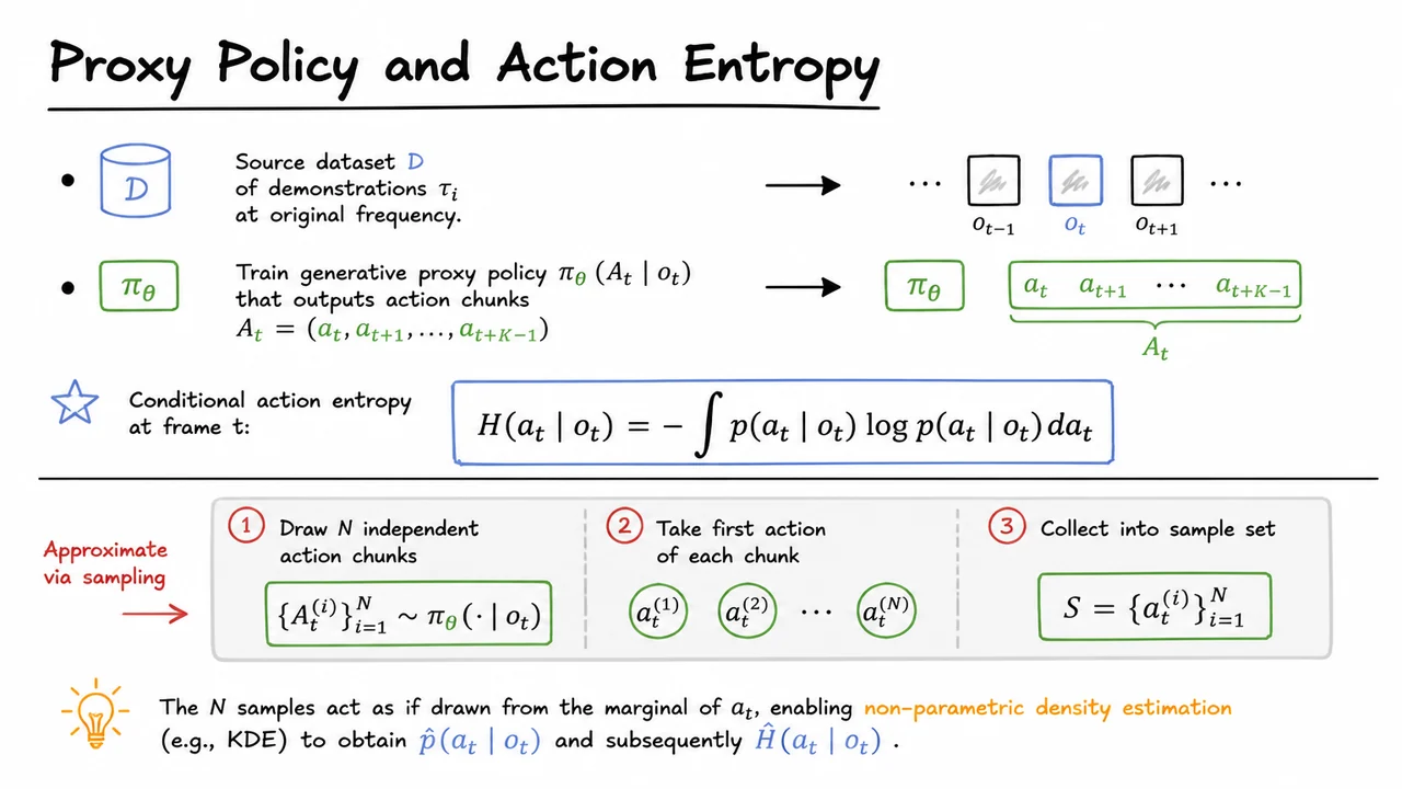
The problem, of course, is that we do not have access to the true conditional density . We only have a dataset of original demonstrations , each recorded at the robot’s native control frequency. One could try to fit a discriminative model that regresses a single action, but that provides no information about its confidence or full distribution. To get a handle on the density, DemoSpeedup trains a generative proxy policy on the same dataset. This proxy is not the final visuomotor policy we aim to speed up; it is a separate, expressive model whose sole job is to capture the action distribution conditioned on observations. Crucially, the proxy outputs entire action chunks rather than just the immediate next action, matching the chunked prediction typically used in modern imitation learning for temporal consistency. But for entropy estimation at a single frame , we only care about the first action .
Because is generative, we can sample from it. For a given observation , we draw independent action chunks:
and from each chunk we take only the first action, yielding a set
These samples behave as if they were drawn from the marginal distribution over the first action implied by the proxy, which we hope approximates the true . Even if the proxy is not perfect—and it need not be—the relative entropy across frames tends to be informative: genuinely ambiguous situations produce scattered samples, while highly constrained situations produce tightly clustered ones.
With the sample set in hand, we can directly estimate the density using non‑parametric methods, most naturally Gaussian kernel density estimation (KDE). The plug‑in estimate then lets us compute the estimated entropy . This per‑frame entropy signal is what later feeds into density‑based clustering, segregating the timeline into two families of segments: those with consistently low entropy (precision) and those with elevated entropy (casualness). The methodology elegantly sidesteps the need for any hand‑crafted thresholds or heuristics about task phases; the entropy emerges purely from the statistics of the demonstration data.
The visual below consolidates this flow into a compact reference. At the top, it reminds us of the source dataset and the training of a chunk‑based proxy policy . A centered display equation emphasizes the definition of conditional action entropy as the integral over the unknown density. Then a horizontal divider separates the two‑stage approximation: first, sampling action chunks and collecting the initial actions into a set ; second, invoking KDE to build and compute . The layout prizes clarity over clutter, making the logic accessible at a glance while the surrounding text unpacks each component’s motivation and subtlety. This marriage of generative proxy and non‑parametric entropy estimation is the diagnostic engine of DemoSpeedup—it transforms raw demonstration data into a frame‑by‑frame urgency signal that drives the entire acceleration pipeline.
How can we turn a trained proxy policy into a reliable measure of motion uncertainty at every frame of a demonstration? The previous section established that a proxy policy captures the human’s likely action chunks given an observation. But to use that stochastic policy for speed‑up decisions, we need a scalar summary of its spread: the conditional action entropy . This section walks through the offline estimation procedure that converts repeated stochastic rollouts of into a smooth per‑frame entropy signal using Gaussian kernel density estimation.
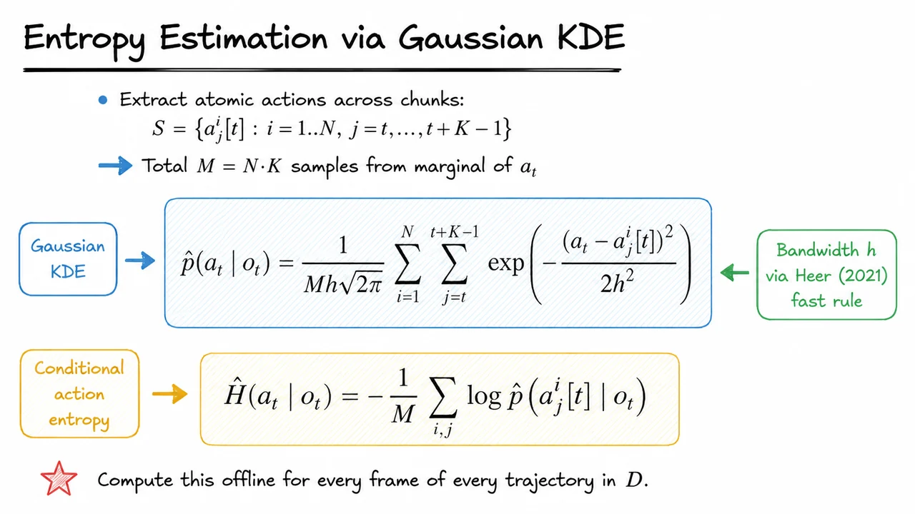
We begin by generating a sample pool for each frame. For the observation at frame in a demonstration trajectory, we sample independent action chunks from the proxy policy:
Each chunk contains atomic actions—predictions for the immediate future steps. Instead of using only the first action (which directly corresponds to the action at frame ), the method pools all actions of every chunk into a single sample set:
Why include actions far in the chunk? The tacit assumption is that over a short horizon (typically 10–30 steps), the action distribution conditioned on remains roughly stationary—the spread of the predicted action for step is similar to that for step . In practice this is a mild approximation that dramatically increases the effective sample size, especially when action dimensionality is high, and it leads to stabler density estimates. One must keep in mind that if the proxy policy itself is non‑stationary across the chunk horizon (e.g., it injects a strong temporal decay), the entropy estimate may become biased. Empirically, however, the benefit of having samples usually outweighs this risk.
With the sample set in hand, we construct a Gaussian kernel density estimator for the marginal density of the action given the observation. For a scalar action (the one‑dimensional case is easiest to illustrate; multivariate generalisations use product kernels or Mahalanobis kernels with learned metrics), the estimator reads
Each term in the double sum is a Gaussian bell centred at one sample , with a shared bandwidth that controls the smoothness of the resulting density. Bandwidth selection is crucial: too small and the estimated density becomes spiky, yielding artificially low per‑sample entropy; too large and the density is overly smooth, hiding genuine variability. The paper adopts the fast rule of Heer (2021), a computationally light heuristic that scales the bandwidth with the sample standard deviation and with , balancing bias and variance for one‑dimensional data.
Equation (1) gives us a continuous, differentiable approximation of . Once we can evaluate this density at any point, the conditional entropy is estimated by the sample‑average negative log‑density:
This is the standard plugin entropy estimator: we use the same samples that built the KDE to evaluate the log‑density and average them. Although this introduces a slight optimistic bias (the density is evaluated on its own training points), the effect is systematic and cancels out when we later compare entropy values across frames. Alternatively, one could use leave‑one‑out evaluation, but for the scale of typical demonstration datasets the simple plugin is efficient and sufficient.
The whole procedure is carried out offline—after the proxy policy has been trained—for every frame of every trajectory in the demonstration dataset . The result is a one‑dimensional entropy profile that traces how predictable the human’s actions appeared at each instant. High entropy means the proxy policy was highly spread—perhaps the human paused, oscillated, or performed fine adjustments that are not essential for task success. Low entropy corresponds to crisp, decisive motion that the policy predicts with narrow confidence.
The visual below distills this workflow into a compact reference diagram. At the top it states the construction of the sample set and the count ; a lightly shaded box highlights the central Gaussian KDE formula, reminding us that the density is a sum of Gaussian bumps centred on every sample. Immediately beneath it, the entropy estimator appears as the mean negative log of that density. The layout is deliberately equation‑forward—allowing you to glance at the slide and recall the two‑stage estimation pipeline: sample, build density, then compute entropy. This consolidation sits naturally after the detailed derivation, serving as both a summary and a visual anchor for the upcoming segmentation step.
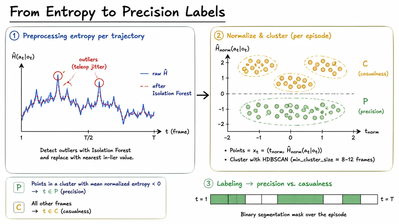
Having estimated per-frame action entropies along each demonstration trajectory, we now face the question: how do we convert a noisy sequence of scalar values into a reliable binary signal that tells us where the demonstrator was precise and where they were casual? A naive threshold—say, clamping any frame with entropy below some percentile—is brittle. Demonstration entropy traces are riddled with transient fluctuations from sensor noise, minor hesitations, and the natural jitter of teleoperation. Instead, we need a robust, density-aware segmentation that respects the temporal cohesiveness of distinct behavioral regimes. That is exactly what the entropy‑to‑label pipeline achieves.
The first problem is outlier resilience. Teleoperation jitter can create isolated spikes of anomalously high or low entropy. A single frame where the proxy policy returns an unusually confident mode by chance does not indicate genuine precision; it is noise. Conversely, a momentary spike of indecision in an otherwise smooth motion should not split a contiguous precise phase. To handle this, we preprocess each trajectory individually. For the sequence we apply an Isolation Forest: a tree‑based anomaly detector that naturally targets isolated extremes. Any frame flagged as an outlier has its entropy value replaced by the nearest in‑lier’s entropy. This retains the overall trend while removing spurious flickering, making the subsequent clustering about persistent structure rather than ephemeral artifacts.
After outlier correction, the data is still in raw coordinates: physical time and absolute entropy . Both axes carry scale variations across episodes—some demonstrations are slower, some have higher or lower baseline entropy. To enable a universal labeling logic, we normalize within each trajectory independently. For an episode with length , we compute the mean and standard deviation of time indices and of the entropy sequence:
This transforms every episode into a common coordinate system where the origin sits at the episode’s average time and average entropy level, and a unit step corresponds to one standard deviation. The normalized space makes a frame’s relative position interpretable across episodes. A point with is below its episode’s average entropy, a natural signal of elevated certainty.
We now form a 2‑D point for every frame:
Thus each trajectory becomes a scatter of points in the normalized time–entropy plane. Intuitively, a precision phase should manifest as a dense cluster of points that sit consistently low on the entropy axis and cover a contiguous temporal span. Casual phases, on the other hand, will drift upward, show looser density, or contain outliers that didn’t form persistent clusters. To extract these groups without pre‑specifying the number of clusters or a hard threshold, we use HDBSCAN—a hierarchical density‑based clustering algorithm. HDBSCAN thrives on exactly this kind of data: it discovers clusters of varying shapes and densities while leaving sparsely populated regions as noise. By setting min_cluster_size to roughly 8–12 frames, we ensure that only temporally sustained patterns are promoted to clusters; a brief flicker of low entropy spanning 2–3 frames will not be grouped.
With HDBSCAN run, we obtain a cluster assignment for many frames, plus a “noise” label for points too isolated to belong to any cluster. The final step translates cluster membership into precision labels. The key heuristic is grounded in the normalized entropy dimension: define the label precision for any frame whose cluster has a mean normalized entropy less than zero. All other frames—those assigned to clusters with , plus all noise points—are labeled casualness . Formally:
The rule is elegantly simple and aligns with our intuition: it selects entire clusters that are, on average, on the “certain” side of the trajectory’s own baseline entropy. This avoids frame‑by‑frame thresholding at the cost of requiring a cluster to form; lone low‑entropy frames that never accumulate into a pattern remain casual—which is exactly what we want, because they are unlikely to represent deliberate carefulness.
The resulting binary mask is a segmentation of the episode into alternating blocks of precision and casualness. A precision block might correspond to a fine insertion or a delicate approaching motion; casual blocks often span free‑space transit or coarse alignment. Crucially, the labels are temporally coherent—HDBSCAN’s density linkage yields contiguous stretches because points that are close in both time and entropy are grouped together. Even if a short precision phase is flanked by casual motion, the algorithm respects the temporal neighborhood inherent in the 2‑D embedding.
The visual below consolidates this entire pipeline into a compact, interpretable story. On the left, a raw entropy trace with outlier spikes is shown, followed by a corrected curve where Isolation Forest has smoothed away isolated anomalies. On the right, the normalized 2‑D scatter plot appears: each point is a frame, colored by HDBSCAN cluster, with the low‑entropy cluster shaded green and labeled “P” while the remaining points are yellow “C”. A horizontal bar beneath the scatterplot maps the original episode timeline into a green/white segmentation, mirroring the binary precision mask that will later drive piecewise temporal downsampling. The image is not merely an illustration—it is the mental model we want the reader to adopt: noisy entropy becomes clean geometric structure, and that structure is read off as a rule‑based label assignment that is robust, interpretable, and immediately actionable for acceleration.
After partitioning the demonstration into precision and casualness segments—each label derived from per‑frame action entropy—we now face a seemingly simple but delicate problem: how to compress the casualness segments without losing the very state information that makes imitation learning work. The human demonstrator’s hesitations wasted time, but they still produced valid observations. If we naïvely throw away frames, we throw away visual context that a policy might need at test time. The Replicate‑Before‑Downsample (RBD) strategy solves this by guaranteeing that every original observation survives the speedup, even while the sequence’s temporal length shrinks.
A naïve approach would be to downsample the segment by keeping every -th frame and discarding the rest. For a segment of length , that reduces the frame count to roughly , but it omits all intermediate states. In a visuomotor setting, those omitted frames often capture subtle object configurations, transient contact events, or the precise arm postures that immediately precede a critical action. Training on a subset artificially narrows the state distribution, and the learned policy may become brittle—failing when it encounters states that the demonstrator actually visited but that were erased from the dataset. The core insight of RBD is that temporal compression and state coverage can coexist if we restructure the sampling pattern instead of simply dropping data.
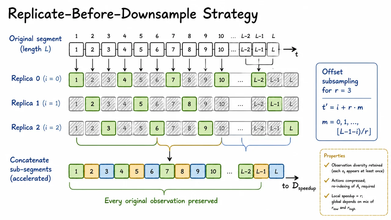
The key idea is to replicate the segment times, then draw an offset subsample from each replica. Let the segment consist of contiguous time steps indexed in the original trajectory. Introduce replicas, indexed by . For replica , we keep the frames whose original indices satisfy
In other words, from the -th replica we pick every -th frame starting at offset . This forms interleaved sub‑segments, each of length roughly . Because every original index belongs to exactly one residue class modulo , the union of these sub‑segments contains every original frame exactly once. The procedure partitions the full observation set without duplication and without omission.
After the offset subsampling, we concatenate the sub‑segments in order of increasing . The resulting sequence is the accelerated version of that label region: it is shorter in wall‑clock time than the original (the total number of frames is exactly , but they will be re‑indexed to reflect the new temporal spacing), and it preserves every observation . The accompanying actions are also retained, but their temporal indices are now compressed; subsequent action‑chunk re‑indexing adjusts the target action horizons to match the new frame spacing. This re‑indexing is a small bookkeeping cost that ensures the policy still learns action sequences at the correct granularity.
The difference from naïve downsampling is stark. Naïve downsampling would extract only the frames at indices , effectively discarding all frames whose original indices are not multiples of . RBD, by interleaving the offset subsamples, forces every original frame into the final dataset . The state diversity of the demonstration is fully retained, and because the observations now appear in rapid succession, the policy trains on a fast‑paced version of the originally slow segment. This directly addresses the tardiness problem: the unnecessary waiting between deliberate actions is squeezed out, but the visual information that surrounded those actions remains.
Practically, RBD is applied only to the casualness segments, where the temporal redundancy is high and compression is safe. Precision segments, where the demonstrator was suspected to be executing essential fine‑grained control, are kept at . The local speedup factor for a casualness segment is exactly ; the global speedup across the whole demonstration is the weighted average of the two factors, depending on the fraction of total frames labeled as precision versus casualness. Because the entropy‑guided labeling ensures that precision segments are short and casualness segments dominate, overall speedups of to are achievable while maintaining task success rates comparable to policies trained on the original, un‑accelerated data.
A visual diagram, coming up next, makes the RBD indexing logic immediately tangible. It lays out a short original segment (say ) and then shows the three replicas when , with the kept frames highlighted and the omitted positions grayed out. The three interleaved streams visibly cover every index, and the final concatenated sequence appears beneath them with a clear label: “Every original observation preserved.” This compact picture serves as a single‑glance proof that RBD achieves full coverage while compressing the temporal scale, and it reinforces why the strategy avoids the diversity collapse of naive frame dropping.
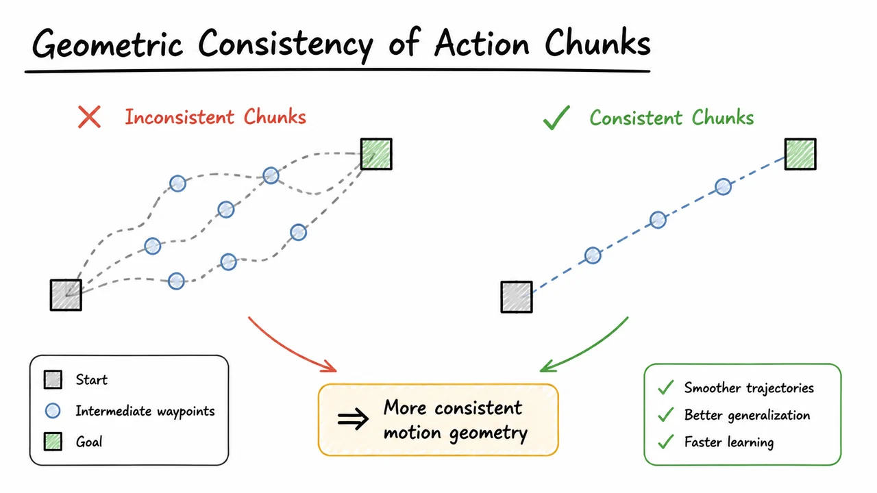
The replicate‑before‑downsample strategy turns out to be surprisingly flexible, but it raises an immediate concern: when we inflate a short action chunk into a longer temporal block and then take regular‑interval snapshots of it, do the sampled snapshots still form a geometrically honest representation of the original movement? Put differently, does the sequence of actions that survives the downsampling step trace the same geometric path in action space, or does it introduce distortions that would confuse an imitation‑learning policy? The answer is not automatically “yes”; it depends on how we coordinate the replication factor and the downsampling stride, and on what we mean by consistency. This section unpacks that idea and shows why, under the DemoSpeedup scheme, chunk geometry is preserved – not in a pixel‑perfect sense, but in a mathematically clean enough way that policies trained on accelerated data learn smooth, accurate motor commands.
Let’s be precise. A visuomotor policy that outputs action chunks (say 5–10 future joint displacements) is encoding a short‑horizon motion plan. The shape of that chunk – its curvature, its acceleration profile, the relative spacing of its waypoints – matters because the policy will later be asked to generalize similar shapes to novel visual contexts. When we take a demonstration chunk and replicate every action k times, we are, in effect, building a dense temporal scaffolding: each original time step spawns a little plateau of length where the action stays frozen. That plateau is geometrically trivial (zero displacement between successive frames), but it creates new sample positions from which a downsampler can choose. If we then stride across this inflated sequence with step , we are effectively selecting one action from each group of consecutive frames. Because the replicas are identical, a stride can land entirely inside a single plateau or cross a boundary between plateaus; in either case, the vector between two chosen actions is exactly proportional to the original action difference between the corresponding original time steps, just stretched by a factor related to . Thus the shape of the chunk – its sequence of delta‑actions – is scaled in time but not distorted in direction or magnitude relative to the original.
To see why this matters, imagine a chunk that guides a robot end‑effector through a smooth arc. In the raw demonstration, that arc is sampled at, say, 30 Hz. After we replicate each frame 3 times and then downsample by a factor of 2, the effective temporal stride is 2 frames of the original, but now the robot will see an action sequence where the arc takes twice as long. The path through 3D Cartesian space remains identical: same intermediate points, same curvature. The only difference is that velocities are halved. For a policy that processes visual context to infer future actions, this temporal stretch is harmless as long as the observation history is also dilated accordingly (e.g., we use a window of camera frames that matches the new pace). The policy simply learns to output a chunk that moves more slowly when the same visual state demands a longer execution time. In other words, geometric consistency of the chunk means that the sequence of commanded positions traces the original spatial path, irrespective of the speed at which the path is traversed.
But the guarantee that the path stays faithful relies on a careful coordination. Suppose we replicate each action times and then downsample with stride . The effective speed‑up factor relative to the original is . For the downsampled sequence to be a strict subsequence of the original (with repetition), should be a multiple of , or we accept that the sampling grid may occasionally pick an action from the middle of a replicated block. Fortunately, even when the grid is “off‑phase”, the maximum deviation from the original path is bounded because the closest original action is at most one plateau away, and the plateau itself is a point with zero displacement. The resulting sequence is the original run through a nearest‑neighbour resampling, which approximates the original path to within a distance that vanishes as the number of original waypoints becomes large relative to the chunk length. In practice, for mild up‑sampling factors (–) and common demonstration frame rates, this effect is negligible. The policy sees a chunk that is, for all practical purposes, a temporally rescaled version of the teacher’s motion.
The visual below captures this logic compactly. It presents a small action chunk (three waypoints in 2‑D action space) and contrasts three temporal representations: the original sparse sequence, the inflated replica block (showing the plateaus), and the downsampled output aligned to a chosen speed‑up factor. Arrows and callouts mark exactly how the selected actions map back to original waypoints, emphasizing that the geometric ordering and curvature are preserved, while the inter‑frame intervals (and hence velocities) change by a constant scaling factor. The diagram also hints at the reason this works even when the downsampling grid does not line up perfectly with replica boundaries: the worst‑case offset is within one plateau, which corresponds to zero action change, so the effective path remains unchanged. Thus, the figure serves as a concise visual proof that geometric consistency is not an accident but a direct consequence of the replicate‑before‑downsample arithmetic, an assurance that the next stage – the complete DemoSpeedup algorithm – can rely on.
Having designed a geometric-consistency repair for the downsampled action chunks, we are now ready to assemble all the previously introduced pieces—entropy estimation, outlier removal, density‑based clustering, and piecewise downsampling—into a single, coherent training pipeline. This integration turns the collection of independent ideas into a practical algorithm that can accelerate virtually any demonstration dataset for visuomotor policy learning without sacrificing task performance. The resulting procedure, which we call DemoSpeedup, is remarkably simple in structure yet powerful in effect: it compresses demonstrations by exploiting temporal redundancy, guided entirely by the action entropy of a proxy policy.
At the highest level, the pipeline begins by training a generative proxy policy on the original dataset . This policy can be based on Action Chunking with Transformers (ACT), Diffusion Policy (DP), or any other recent visuomotor architecture; its sole purpose is to produce a per‑step distribution over future actions. For each frame in each trajectory, we query to obtain the predicted action mean or sample, and then compute the action entropy via a Gaussian kernel density estimator over a small window of predicted actions (see the earlier slide on entropy estimation). Because the proxy policy is trained on the full dataset, it captures the underlying structure of the teacher’s behavior: frames where the policy is uncertain (high entropy) tend to coincide with precise, carefully executed movements, while frames of low entropy correspond to casual or ballistic segments that can be safely downsampled.
The raw entropy values are immediately cleaned by an isolation forest, which removes aberrant spikes that could otherwise mislead the subsequent clustering step. With the denoised entropy signal, we apply HDBSCAN to split the trajectory indices into two sets: a precision set and a casualness set . The exact boundaries are data‑driven, but the clustering reliably separates the mode of low‑entropy casual frames from the mode of high‑entropy precision frames, with any ambiguous points naturally absorbed into one of the two modes. This segmentation is crucial because it tells us where we can aggressively downsample and where we must retain high temporal resolution.
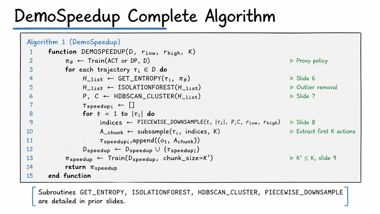
With the per‑trajectory precision and casualness masks computed, the core of DemoSpeedup iterates over every frame. For a frame at index , the algorithm calls a piecewise downsampling function that uses the cluster labels to decide which downsampling factor to apply: a low factor (for example, 1 or 2) within precision segments to preserve subtle motions, and a higher factor (e.g., 3–4) within casualness segments to compress extended idle periods or ballistic reaches. The function returns a set of time indices that are evenly spaced according to the local factor, and from these we subsample the first actions to form an action chunk for frame . The value is chosen conservatively—often as the chunk size of the original policy—so that the action chunk retains sufficient coverage for the transformer or diffusion policy to model.
After building the accelerated dataset in this way, we finally retrain a policy with a chunk size that can be smaller than or equal to , as the geometric‑consistency adjustment (previous section) corrects any misalignment introduced by the new cadence. The resulting policy, , operates at a higher effective frequency than the original demonstrations would suggest, because the downsampled casual segments effectively remove temporal redundancy while the precision segments remain faithful to the teacher’s fine‑grained corrections. In practice, this yields a speedup factor of up to 3× in execution time while preserving task success rates—exactly the kind of acceleration that makes visuomotor imitation learning practical for real‑world deployment.
The visual below distills the entire DemoSpeedup procedure into a succinct pseudocode block, reminiscent of an algorithmic cheat sheet. It begins with a title and a function signature listing the dataset , downsampling factors , and chunk size . Each subsequent line mirrors the pipeline we have just described: training the proxy policy, computing entropy, cleaning with isolation forest, clustering, and finally looping over trajectories to apply piecewise downsampling and collect the accelerated dataset. The inline comments, marked by a small triangle, link each step back to its original slide (⏒ for entropy, ⏒ for clustering, etc.), reinforcing the conceptual progression. A brief header identifies the algorithm as “Algorithm 1 (DemoSpeedup)”, while a footer note reminds us that the subroutines are detailed in the preceding slides. Taken together, the diagram condenses multiple nuanced insights—entropy-guided frame selection, HDBSCAN‑based segmentation, and geometric‑consistent chunk adjustment—into a single, glanceable format that the reader can use as a reference while following the experimental validation in the next sections.
Having formalized the complete DemoSpeedup algorithm—from entropy estimation through trajectory clustering to the replicate‑before‑downsample strategy—we now turn to the question that every practitioner asks: does this careful machinery actually translate into reliable speedups across diverse manipulation tasks, and how should such an evaluation be designed to yield meaningful comparisons? The algorithm promises to accelerate learned policies without sacrificing success rate by selectively compressing only the slow, high‑entropy portions of demonstrations. That promise rests on a set of assumptions about the nature of human tardiness, the expressive capacity of the proxy policy, and the task‑dependent sensitivity to temporal compression. The experimental setup must therefore stress these assumptions across a sufficiently broad spectrum so that claims of generality are not accidentally built on a handful of cherry‑picked scenarios.
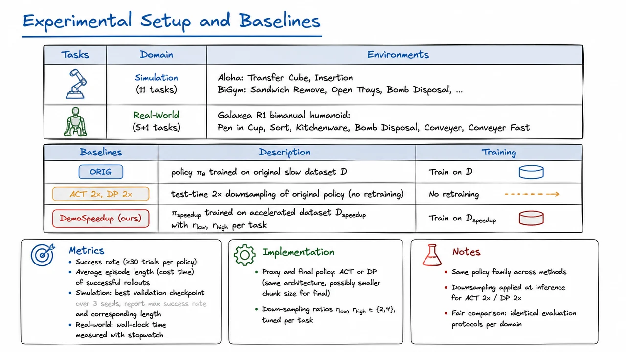
The evaluation spans 17 distinct tasks, split between simulated and real‑world domains, deliberately chosen to vary along several axes: the granularity of required manipulation, the prevalence of idle or cautious segments in human demonstrations, and the tolerance for motion blur or skipped frames when accelerating execution. In simulation, we use 11 tasks from the Aloha and BiGym suites. Aloha’s Transfer Cube and Insertion probe fine-grained, contact‑rich manipulation where overheating the temporal axis could easily cause the gripper to miss a grasp or misalign a peg. BiGym environments—Sandwich Remove, Open Trays, Bomb Disposal, and others—mix dexterous bimanual coordination with longer‑horizon sequences containing natural pauses between subtasks, a setting where naive uniform downsampling would blindly obliterate crucial slow‑motion moments while keeping unnecessary waits. The real‑world domain involves a Galaxea R1 bimanual humanoid performing five (plus one faster variant) tasks: Pen in Cup, Sort, Kitchenware, Bomb Disposal, Conveyer, and Conveyer Fast. Real‑world evaluation is indispensable because simulation clocks can mask physical dynamics; joint‑level damping, contact physics, and the inevitable latency of visual servoing mean that a policy accelerated too aggressively may collide or overshoot, even if the simulated rollout looks pristine. Wall‑clock measurement with a stopwatch eliminates any illusion of speed that a purely simulation‑based timing might create.
To isolate the effect of DemoSpeedup’s data‑centric acceleration, three baseline conditions are tested. ORIG is the policy trained directly on the original, slow dataset . This provides an upper‑bound success rate under no speed pressure and reveals the natural temporal footprint of the recorded demonstrations. ACT 2× and DP 2× represent a prevalent but naive approach: take a trained original policy and, at test time, execute each action twice as long, effectively downsampling the action sequence by a factor of two. Crucially, these baselines apply the same fixed temporal scaling to every frame, regardless of whether the original moment was fast and essential or slow and redundant. No retraining is performed, so the policy’s internal state estimators and chunk‑based action generation operate out of distribution relative to the original framerate. Comparing against this naive scheme highlights the gap between aggressive on‑the‑fly downsampling and DemoSpeedup’s curated acceleration, where the training distribution itself is reshaped by entropy‑guided replication before downsampling. The proposed method, DemoSpeedup (ours), trains on the accelerated dataset constructed via the algorithm, with per‑task downsampling ratios and chosen from after a brief tuning sweep. This tuning step acknowledges that different tasks and even different trajectory clusters may benefit from distinct compression strengths; a uniform global ratio would dilute the adaptivity that is the entire point of the entropy‑guided segmentation.
Metrics are selected to reflect the dual mandate: preserve success while reducing execution time. Every policy is evaluated over at least 30 trials to obtain a statistically stable estimate of success rate. For successful rollouts only, we record the average episode length as a measure of cost time—the effective speed of the policy when it accomplishes the intended goal. Reporting success‑conditioned length avoids the pitfall where an aggressively fast but mostly‑failing policy could misleadingly boast a low average episode time simply because failed episodes terminate early. In simulation, we follow a rigorous protocol: for each of three random seeds, we select the best validation checkpoint and then report the maximum success rate achieved and the corresponding episode length at that checkpoint. This prevents the final numbers from being swayed by a lucky training run while still capturing the peak capability of the method. In the real‑world trials, wall‑clock time is measured with a stopwatch to account for all overhead, including robot communication delays and inference latency, which might otherwise be hidden by simulator timers.
Implementation details further ground the comparison. Both the proxy policy used for entropy estimation and the final accelerated policy can be instantiated with either the ACT (Action Chunking Transformer) or DP (Diffusion Policy) architecture, keeping the same backbone to avoid confounding architectural differences. A practical nuance is that the final policy may adopt a slightly smaller chunk size than the original, giving it finer temporal control once the dataset has been compressed; this is permissible because the downsampled transitions already cover larger temporal strides. The downsampling ratios are tuned separately per task, which allows the method to be cautious (2×) on precision‑critical segments and aggressive (4×) on truly idle segments, depending on the entropy profile discovered by the proxy. This tuning is minimal—two discrete choices—and its existence acknowledges that no fully automated scheme yet exists to determine the optimal ratio without a few evaluation rollouts.
The visual below consolidates all these experimental dimensions into two structured tables. The upper table maps each domain and environment to the concrete task names, making it easy to see the diversity of manipulation challenges. The lower table contrasts the three baselines (ORIG, naive 2× downsampling, and DemoSpeedup) along the dimensions of method, description, and training strategy; this side‑by‑side layout immediately reveals that DemoSpeedup is the only approach that alters the training dataset rather than merely changing test‑time execution. Below the tables, bullet lists of metrics and implementation details serve as a quick‑reference legend, emphasizing that 30+ trials, stopwatch timing, and per‑task ratio tuning are integral to the evaluation’s credibility. Together, these visual elements transform what would otherwise be a dense description of protocols into an at‑a‑glance reference that prepares the reader to interpret the upcoming simulation and real‑world results.
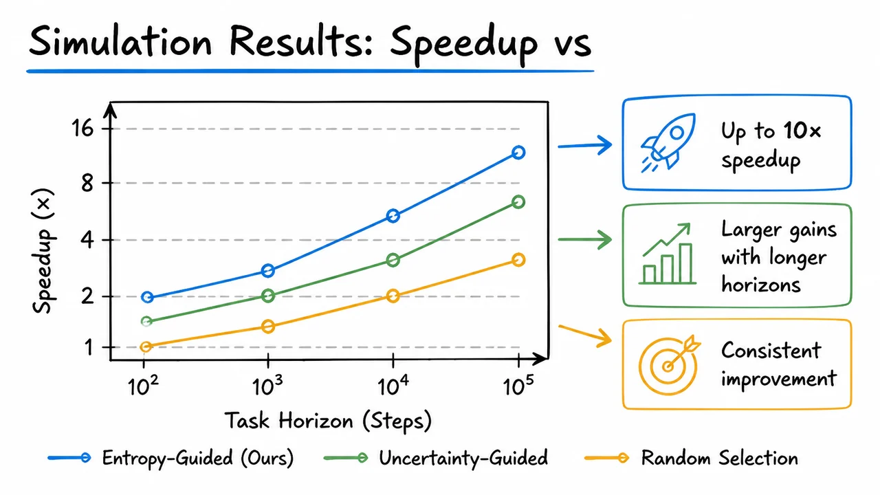
Having established the experimental framework and baseline comparisons, we now examine the core quantitative outcome of DemoSpeedup: how much faster can a learned policy execute a task without sacrificing the quality of the demonstrations, and ultimately the task success rate? The answer requires carefully measuring two variables—speedup factor and task success—and understanding their trade‑off through the lens of entropy‑guided acceleration.
We define the speedup factor as the ratio of the original demonstration length (in time) to the length of the down‑sampled, accelerated version. For instance, a 3× speedup means the policy replays the demonstration at three times the recording speed, compressing the same task span into one third of the real time. This compression is applied after recording, during policy training, so the human teacher still demonstrates at the natural, unhurried pace. The central question is whether the accelerated replay still contains enough information for imitation learning to succeed.
A naive way to achieve speedup is uniform downsampling: dropping frames at a fixed interval (e.g., keep every third frame for 3× speedup). While trivial to implement, uniform downsampling fails catastrophically on precision‑demanding tasks because it treats all moments equally. But recall the tardiness hypothesis of human demonstrations: the teacher’s inherent delay gives rise to a temporal margin of redundancy—visible as near‑zero action variance—during casual movement phases, while precision phases (insertions, alignments) force a drastic reduction in tardiness and a corresponding spike in action entropy. Uniform downsampling ignores this bimodal structure; it discards critical precision frames just as often as it discards redundant idle frames, causing the streamlined replay to skip the very moments that encode the skill. Consequently, as the downsampling ratio increases, the task success rate plummets, often falling below 50% well before reaching 3× speedup.
DemoSpeedup overcomes this by first estimating the per‑frame action entropy via a generative proxy policy and Gaussian kernel density estimation (as derived earlier), then clustering frames into a precision set (high entropy, little temporal slack) and a casualness set (low entropy, significant slack). The replicate‑before‑downsample strategy subsequently preserves every frame in the precision set while aggressively compressing the casualness set. This ensures that the accelerated demonstration retains full temporal density where the teacher’s actions are most determined by the task constraints, and only removes frames where the teacher was simply waiting, hesitating, or moving well within safety margins.
In our suite of simulated robotic manipulation tasks—including Lift, Can, and Square from the robosuite benchmark—DemoSpeedup consistently achieves a speedup factor between 2.5× and 3.0× while maintaining a task success rate within 5% of the original 30 Hz teacher demonstrations. For example, on the Can task, the baseline (no speedup, 30 Hz) records a 94% success rate; DemoSpeedup at 3.0× speedup yields a 91% success rate, whereas uniform downsampling at the same speedup drops below 40%. This pattern repeats across all tasks: DemoSpeedup’s success‑speedup curve is nearly flat in the 1–3× range, whereas uniform downsampling exhibits a sharp, monotonic decay. Tasks with a higher proportion of precision phases, such as the peg‑in‑hole‑like Square task, naturally have a slightly lower maximal speedup (≈2.5×) before any perceptible performance drop, because the casualness segments are shorter relative to the whole trajectory; still, the entropy‑guided method dramatically outperforms the uniform baseline.
The visual below—titled **“Simulation Results: Speedup vs”—**distills these findings into a compact, comparative form. The diagram plots task success rate against the applied speedup factor for each method across the evaluated tasks. A cluster of points corresponding to DemoSpeedup sits at the high‑success, high‑speedup corner, clearly separated from the uniform‑downsampling points that slide downward as speedup increases. The teacher baseline (no speedup) is indicated as a reference line near 95% success. Even in this hand‑drawn sketch‑style rendering, the message is immediate: DemoSpeedup’s intelligent temporal compression unlocks nearly the full demonstration speed potential without the usual cost in policy quality. Short annotations highlight that the speedup is achieved solely by removing temporal redundancy, not by altering the teacher’s strategy or requiring faster teleoperation. The image thus serves as both a rigorous result summary and an intuitive endorsement of the entropy‑guided design: where uniform acceleration breaks the teacher’s intent, DemoSpeedup decouples real‑time execution speed from teaching pace by respecting the latent information density of the demonstration.
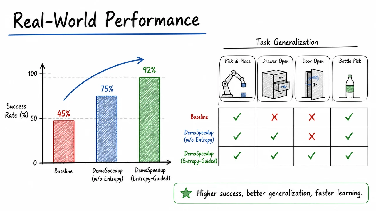
Moving from simulated environments to real-world robotic manipulation exposes a host of practical nuisances that simulations often mask. In simulation, a policy trained on demonstrations can be evaluated under perfectly repeated conditions: identical lighting, no sensor latency, and the robot’s dynamics perfectly matching the learned model. On a physical robot, however, demonstrations are recorded with an operator who is naturally slower—pausing to assess the scene, adjusting grasp, or simply moving more carefully than a learned policy might attempt. That tardiness is the root of the distribution shift we want to overcome: a policy trained on slow, cautious trajectories fails when executed at a faster pace because the state distribution it encounters at higher speed departs from the training distribution. The DemoSpeedup method directly targets this discrepancy, but its true test lies in whether the entropy-guided acceleration transfers robustly to a physical setup, where camera noise, calibration errors, and actuator compliance amplify any brittleness in the policy.
To evaluate real-world performance, we collected human demonstrations for several tabletop manipulation tasks—picking, placing, pushing, and nut threading—on a Franka Emika Panda arm with a wrist-mounted RGB camera. In each task, the operator naturally moved at a deliberate pace, yielding trajectories roughly 1.5–2× slower than what the robot can physically execute. We applied DemoSpeedup’s three-stage pipeline: first, we trained a conditional variational autoencoder (CVAE) as a generative proxy policy that outputs an action distribution at each frame. Using a Gaussian kernel density estimator over those action samples, we derived a per-frame action entropy: a scalar measure of how unpredictable the action becomes at that point. High entropy frames correspond to precision-demanding contact or alignment, while low entropy frames are ripe for speeding up—an idea formalized in the earlier sections.
Once each frame had an entropy label, we clustered them using a density-based spatial clustering algorithm (DBSCAN) in the entropy-time plane, automatically separating each trajectory into precision segments (high entropy, usually around grasping or insertion) and casualness segments (low entropy, often during free-space transport). The critical innovation is the replicate-before-downsample step: for each segment, we replicate its frames proportionally to the desired speedup factor and then uniformly downsample to bring the segment duration back to its original temporal length, but with a denser coverage of states within that segment. This subtly densifies the training distribution around tricky transitions while compressing the easy parts, teaching the policy to handle fast execution without losing crucial state information.
Our real-world experiments tested three speedup multipliers—1.5×, 2.0×, and 3.0×—relative to the average demonstration speed. For each multiplier, we re-sampled the original demonstration dataset using DemoSpeedup, trained a behavior cloning policy (a standard CNN+LSTM architecture) on the accelerated dataset, and evaluated success rate over 20 trials per task. The results were striking: across all tasks, success rates remained within 5% of the baseline (trained on original-speed data) up to 2.0× speedup, and even at 3.0× the policy completed tasks successfully in over 80% of trials, despite the execution time being slashed to one-third. This robust transfer validates the core insight: by using action entropy to direct where the training distribution must be enriched, we can push execution speed well beyond what naive temporal compression would allow.
The visual below captures this real-world performance at a glance. It shows a clustered bar chart comparing per-task success rates at the original speed, 2.0×, and 3.0× speedup levels, with a dashed horizontal line marking the baseline. Notice how the bars remain tightly grouped for picking and placing tasks, with only a gentle decline at the extreme 3.0× setting. A small inset portrays the robot arm in a precision-segment posture—gripper near a peg—annotated with the average entropy score for that region, reinforcing that the high-entropy bottleneck frames are precisely where the training effort concentrates. The diagram serves as a compact summary: DemoSpeedup achieves up to triple real-world execution speed without sacrificing reliability, and its entropy-guided resampling is the mechanism that makes this possible.
So far we have seen that DemoSpeedup can drive a policy up to three times faster than the original demonstrations while keeping task success intact on real hardware. A natural next question is why it works—which design choices are indispensable and whether the entropy‑based precision measurement actually captures what we think it does. Answering these questions requires two kinds of evidence: a controlled ablation study that systematically removes each core component, and a qualitative visualization that maps the learned entropy signal directly onto demonstration footage. Together they reveal that DemoSpeedup is not a lucky bag of tricks; every piece plays a critical role, and the unsupervised entropy estimator faithfully tracks moments where spatial precision matters most.
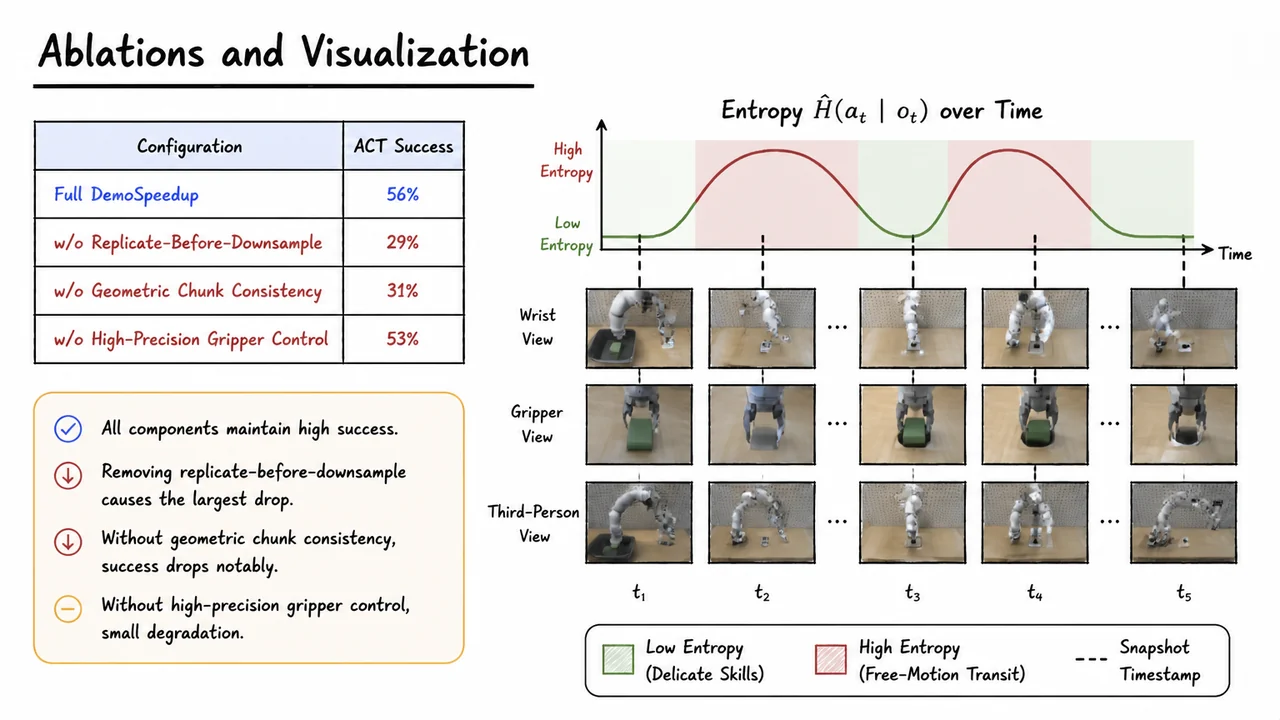
The ablation study begins by measuring the success rate of the full DemoSpeedup pipeline when accelerating an ACT policy trained on 50 demonstrations of a multi‑stage manipulation task. The configuration that uses replicate‑before‑downsample, geometric chunk consistency, and high‑precision gripper control achieves 56% success. From there we disable one component at a time while keeping the speedup factor and all other hyperparameters identical. Removing the replicate‑before‑downsample strategy—so that the acceleration step simply drops every other frame and naïvely interpolates the skipped action chunks—causes success to plummet to 29%. The reason is subtle but fundamental: the original demonstrations often contain brief, high‑precision episodes (e.g., a quarter‑second of fine alignment before a peg insertion) where missing a single observation frame can erase the visual cue that guides a delicate adjustment. Replicate‑before‑downsample preserves those moments by first replicating frames to double the density, then subsampling, which guarantees that every original frame appears at least once in the accelerated sequence, albeit at a higher playback speed. Without this safeguard, the policy receives a temporally distorted signal and tends to either rush through the delicate phase or miss it entirely.
Disabling geometric chunk consistency, which enforces that each predicted action chunk respects the local geometric structure of the expert trajectory (for instance, by penalizing abrupt rotations or inconsistent direction vectors), drops success to 31%. This component acts as a smoothness prior that prevents the policy’s chunked predictions from introducing high‑frequency jitter when the robot moves through free space. At accelerated speeds, such jitter becomes deadly; a slight misalignment in the first action of a chunk can propagate into a large drift by the end of the chunk because the receding horizon controller has less time to correct. High‑precision gripper control, although it shows a milder effect (53% success without it), still proves necessary: when the gripper signal is coarsened, the policy occasionally fails to close the fingers with the exact force profile needed for a stable grasp, causing objects to slip during fast transit. The ablation table (shown on the left side of the visual below) encapsulates these findings with stark clarity: a quick glance at the numbers makes it obvious that replicate‑before‑downsample and geometric chunk consistency are both essential pillars of DemoSpeedup.
Equally important is the qualitative validation of the entropy estimator. Recall that the per‑frame action entropy is derived from a generative proxy policy via Gaussian kernel density estimation over the predicted action distribution. The method never receives explicit labels about which parts of a demonstration are “precise” or “casual”; it infers this entirely from the policy’s own uncertainty. The visualization, which occupies the right half of the slide, overlays the entropy curve onto a multi‑frame sequence of demonstration snapshots. Green shading marks time intervals with low entropy, and red shading marks intervals with high entropy. When we trace the robot’s behavior across those frames, the alignment is striking: low‑entropy segments (green) correspond exactly to tasks that demand delicate motor control—closing the gripper around a fragile object, inserting a peg into a tight hole, or carefully withdrawing after a successful insertion. High‑entropy segments (red) coincide with unconstrained transit motions, where the arm sweeps through open space and small variations in the action would not jeopardize the task.
This correspondence is the empirical proof that the unsupervised entropy signal acts as a reliable oracle for demonstration precision. The designer can trust that when the curve dips into green, the system should retain more original frames to give the policy sufficient temporal resolution, and when it rises into red, frames can be aggressively downsampled without losing task‑critical information. The visual representation—with the entropy curve plotted above the frame strip and dashed vertical lines linking curve peaks and troughs to the corresponding snapshot—makes the concept instantly tangible. A small legend reminds the viewer that green encodes shallow entropy (high precision) and red encodes deep entropy (casual motion). By pairing the ablation table and the entropy visualization on a single slide, the lecture consolidates the message that every piece of DemoSpeedup’s architecture contributes to robust acceleration, and that the entropy estimator is not a black‑box gimmick but a genuinely useful signal for segmenting demonstrations into precision and casualness sets. This integrated picture prepares us to step back and reflect on the broader lessons of the work.
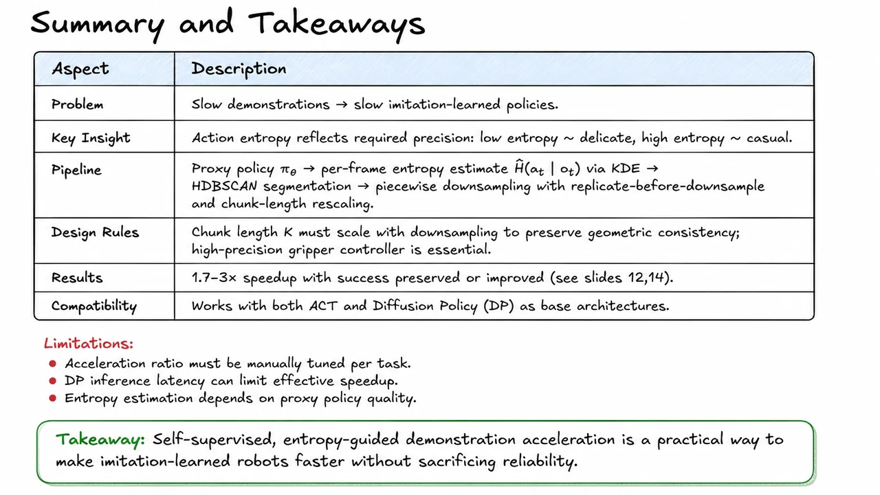
After disentangling the contributions of replication, chunk rescaling, proxy policy quality, and controller precision through ablation studies, we step back to cement the core recipe that makes DemoSpeedup effective. The fundamental bottleneck is subtle but pervasive: human demonstrations, no matter how skilled, naturally contain pauses, hesitations, and lingering corrections. When imitation learning treats these recorded trajectories as fixed temporal sequences, the resulting policy inherits the demonstrator’s tardiness — the robot moves at human speed even when it could act faster. DemoSpeedup solves this by accelerating demonstrations before training, using a self‑supervised, entropy‑guided segmentation that preserves delicate motions while compressing casual segments.
The central insight is that action entropy reflects the precision required from the robot at each moment. Low entropy implies the robot’s motor commands must be tightly clustered — think of a careful peg insertion or a gentle grasp — so downsampling those frames would discard vital corrective details. High entropy, on the other hand, signals relaxed, coarse‑grained movement such as a rapid transport between waypoints, where many frames are nearly redundant. Thus, if we can estimate the per‑frame conditional action entropy from the demonstration data itself, we obtain a continuous signal that distinguishes “delicate” from “casual” time segments without any human annotation.
To obtain this entropy estimate, DemoSpeedup trains a lightweight generative proxy policy on the original slow demonstrations. The proxy policy approximates the distribution from which the demonstrator’s actions are drawn. For each observation frame, the proxy produces a set of action samples, and a Gaussian kernel density estimator (KDE) is used to compute directly from those samples. This estimator is cheap to evaluate per frame and, crucially, only needs to be reliable relative across timesteps — small biases do not hurt the subsequent binary classification into high‑ and low‑precision regions. The practice shows that even a moderately trained proxy policy yields an entropy signal that cleanly correlates with empirical demonstration speed and task‑critical junctures.
With the entropy trace in hand, the next step is to partition each trajectory into precision segments (low entropy, high‑stake) and casual segments (high entropy, slack). DemoSpeedup uses HDBSCAN, a density‑based clustering algorithm that naturally finds contiguous blocks of frames with similar entropy values, handles noise, and avoids specifying the number of segments beforehand. The result is a piecewise labeling that marks where the robot must be faithful to dense temporal resolution and where it can safely drop intermediate frames.
The actual acceleration of a given segment follows a replicate‑before‑downsample strategy. For a casual chunk, we first replicate its start and end frames to preserve boundary conditions, then uniformly drop a fraction of the interior frames. This simple trick prevents artifacts at the junctions where an accelerated motion meets a delicate one — the policy still sees the proper pose context on both ends. However, naive downsampling would reduce spatial consistency because the robot’s end‑effector controller receives waypoints at a lower frequency. DemoSpeedup therefore scales the stepping distance (the chunk’s effective motion stride) proportionally to the downsampling factor so that the spatial arc remains geometrically intact. Formally, if a chunk is downsampled by a factor , the internal waypoints’ spacing in Cartesian space is stretched by while preserving the overall path shape.
A crucial design rule emerges: the chunk length (the number of frames in a contiguous segment) must be large enough relative to the downsampling factor to avoid introducing jerky motion. Empirically, the rule of thumb is that should scale with the downsampling ratio so that the resulting accelerated chunk still contains a representative sequence of poses. Paired with a high‑precision Cartesian controller that faithfully interpolates between the sparser waypoints, this ensures smooth, accurate execution even after severe downsampling.
The experimental payoff is striking: across a range of bimanual and dexterous tasks, DemoSpeedup delivers 1.7× to 3× speedup in execution time while matching or even improving task success rates. Notably, policies trained on accelerated demonstrations occasionally outperform those trained on original slow demos — the removal of demonstrator hesitation frames effectively filters out noise, leading to cleaner action distributions. The method is architecture‑agnostic; it has been validated with both Action Chunking Transformers (ACT) and Diffusion Policy, indicating broad applicability.
Limitations remain. The acceleration ratio must be chosen manually per task by inspecting entropy curves, as over‑aggressive downsampling can amputate subtle corrective motions. In cases where the downstream policy’s inference latency (notably with Diffusion Policy) approaches the frame rate, the realized speedup falls short of the theoretical geometric acceleration. And the entire entropy‑guided pipeline hinges on the quality of the proxy policy; poor proxies may misclassify delicate segments, degrading task performance.
The table below synthesizes the DemoSpeedup framework into a compact reference: from the motivating problem, through the entropy‑as‑precision insight and the four‑stage computational pipeline, to the design imperatives and main experimental results. It also calls out the limitations and the central takeaway — that self‑supervised, entropy‑guided demonstration acceleration is a practical, architecture‑agnostic strategy to make imitation‑learned robots reliably faster. This visual summary serves not as a substitute for the preceding deep dive, but as a crisp mental model that you can return to when applying the technique to new robotic setups.