Generative modeling sits at the heart of modern machine learning, yet the problem it poses is deceptively simple to state and brutally hard to solve. We are handed a finite collection of observations — photographs, audio clips, protein structures, text documents — and asked to learn the hidden probability distribution that produced them well enough to both evaluate and sample from it. Everything else in this lecture grows out of understanding precisely why that is difficult.
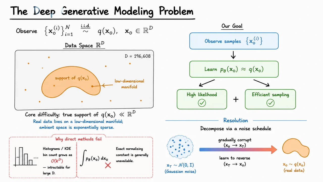
Formally, suppose we observe a dataset , where each . For a standard RGB image at 256×256 resolution, . Our task is to find parameters such that a model distribution satisfies
A useful generative model must satisfy two simultaneous desiderata. First, it should assign high likelihood to real data — meaning should be large wherever is large. Second, it should support efficient, diverse sampling — drawing fresh examples that look indistinguishable from real ones in finite compute time. These two goals are more in tension than they might first appear; many architectures that excel at density estimation are slow to sample from, and vice versa.
The root cause of almost every difficulty is the curse of dimensionality. The most naïve approach to density estimation is a histogram: discretize each dimension into bins, count how many samples fall into each cell, and normalize. The number of cells scales as , so even with bins per dimension and , the histogram has more cells than there are atoms in the observable universe. Kernel density estimation (KDE) fares no better asymptotically — its sample complexity grows exponentially in . The ambient space is simply too large to cover with any finite dataset.
What saves us — partially — is the manifold hypothesis: real data does not spread uniformly over . Natural images, for instance, live on a vastly lower-dimensional manifold embedded in pixel space. Randomly-sampled Gaussian vectors in look like snow; real images occupy an astronomically small corner of that space. This means the effective complexity of the problem is much lower than the ambient dimension suggests — but we have to build a model that discovers and exploits that low-dimensional structure without ever being told what it is.
Parametric models — neural networks, normalizing flows — try to encode this structure implicitly. But a second fundamental obstacle arises immediately: computing the normalizing constant
is generally intractable for flexible models. If we parameterize an energy-based model , for instance, the integral over all of is unavailable in closed form, blocking both maximum-likelihood training and exact sampling. Normalizing flows avoid this by restricting to invertible architectures with tractable Jacobians — an elegant fix, but one that constrains expressivity and is computationally expensive at scale.
The conceptual breakthrough that motivates this entire lecture is a different kind of resolution: rather than trying to model directly, decompose the problem through a noise schedule. We design a process that gradually corrupts a data point into pure Gaussian noise over steps. This forward process is easy and known by construction. The hard distribution is then recovered by learning to reverse this corruption — denoising noise back into data, one small step at a time. Each individual denoising step operates on a nearly-Gaussian local distribution, sidestepping the global normalization problem entirely.
This noise-based decomposition is elegant for several reasons. It replaces one intractable global problem with a sequence of tractable local problems. It naturally exploits the manifold structure of data, because the noising process smoothly interpolates between the sharp data manifold and a featureless Gaussian. And it connects to deep mathematical tools — stochastic differential equations, score functions, and optimal transport — that we will develop carefully throughout this lecture.
The visual below captures both the difficulty and the proposed resolution in a compact diagram. On one side, it depicts the core tension: data lives on a tiny, irregular support within the vast ambient space , while the model must simultaneously achieve high likelihood and efficient sampling from that distribution. On the other side, the noise-decomposition idea appears as a bridge — a continuum connecting structureless Gaussian noise to the rich, structured data distribution. This bridge is exactly the object we will learn to traverse, and building it rigorously is the subject of everything that follows.
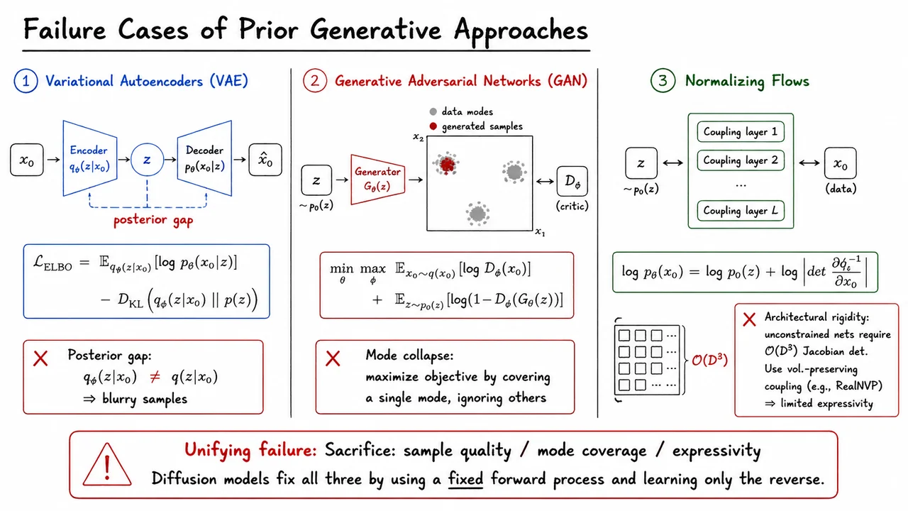
Having established that the core challenge in deep generative modeling is faithfully learning an intractable data distribution from finite samples, it is tempting to ask: haven't we already solved this? Three families of models dominated the field for years — Variational Autoencoders, Generative Adversarial Networks, and Normalizing Flows — and each represents a genuinely clever engineering compromise. The trouble is that each compromise carries a structural flaw that cannot be patched away with more computation or better architecture. Understanding why these flaws are fundamental is exactly the motivation for everything that follows.
Variational Autoencoders take the most principled probabilistic route. The core idea is to introduce a latent variable and optimize a tractable lower bound on the log-likelihood:
The first term rewards accurate reconstruction; the second term regularizes the approximate posterior toward a prior. The critical subtlety is that is a parameterized approximation to the true posterior . Because these two distributions are never exactly equal — a gap that persists at convergence whenever the true posterior is multimodal or has complex geometry — the decoder must effectively average over a smeared-out region of latent space rather than a single precise encoding. This averaging is precisely what produces the notorious blurriness of VAE samples: the reconstruction loss, typically mean-squared error, has the statistical effect of regressing toward the mean of the posterior distribution, washing out sharp high-frequency detail.
Generative Adversarial Networks abandon likelihood altogether in favor of an adversarial game. A generator and discriminator are trained under the minimax objective:
In theory, the unique Nash equilibrium of this game recovers the true data distribution. In practice, the generator can satisfy the discriminator perfectly by placing all of its probability mass on a single sharp mode of . Because the discriminator sees realistic-looking samples and cannot easily penalize the generator for failing to cover the other modes it has never observed, training dynamics fall into mode collapse — a pathology that is both difficult to detect during training and notoriously hard to cure. The fundamental problem is that the generator's objective provides no explicit incentive to maintain coverage of the full data distribution.
Normalizing Flows return to exact maximum likelihood by constructing a sequence of invertible transformations that map a simple base distribution into the data distribution. By the change-of-variables formula:
This is mathematically exact — no approximation, no adversarial game. The problem is computational. For a -dimensional random variable, the Jacobian is a matrix, and computing its determinant naively costs . For images with or , this is completely infeasible. Practitioners must therefore restrict their networks to volume-preserving coupling layers (as in RealNVP or Glow), whose structured form makes the Jacobian triangular and the determinant cheap to compute — but at the cost of severely limiting the expressive power of the transformation. You can have exact likelihoods or expressive architectures, but not both.
The pattern is worth pausing on:
Each method essentially purchases tractability by giving something up. No combination of tricks within any single framework resolves all three problems simultaneously, because each failure mode is a direct consequence of the framework's defining design choice.
Diffusion models sidestep this trilemma through a conceptually different move: instead of designing a clever approximate inference scheme, an adversarial game, or a constrained invertible network, they commit to a fixed, analytically tractable forward process that progressively destroys structure in the data. Because the forward process is given — not learned — there is no posterior gap to approximate, no discriminator to fool, and no Jacobian to compute. The model need only learn to reverse a process whose statistics are fully known. This might sound like it merely pushes the problem elsewhere, but as the next section will show, the reverse process turns out to have exactly the right mathematical structure to be learned efficiently with a simple regression objective.
The visual below consolidates this three-way comparison in a compact side-by-side layout. Each column captures one method's schematic and its critical failure mode — the posterior mismatch in the VAE column, the collapsed generator samples in the GAN column, and the cost annotation on the flow column. The bottom strip unifies all three under a single verdict: in every case, something fundamental is sacrificed. Seeing the three failures lined up in parallel makes it easier to appreciate that diffusion models are not just an incremental improvement on any one approach — they represent a qualitatively different answer to the same underlying question.
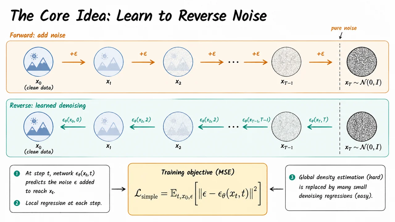
Having established why prior generative approaches struggle — GANs require delicate adversarial balance, VAEs are constrained by their encoder bottleneck, and normalizing flows demand architecturally expensive invertibility — we can now ask a sharper question: is there a way to turn density estimation into something more like ordinary supervised learning? Diffusion models answer that question with a surprisingly elegant reframing.
The key philosophical shift is to stop trying to learn the data distribution all at once. Instead, observe that destroying structure is trivially easy: add a small amount of Gaussian noise to a clean image, and you get a slightly noisier image. Repeat this operation hundreds of times, and the original signal is completely overwhelmed. After enough steps, the distribution of the corrupted sample is indistinguishable from an isotropic Gaussian, regardless of what looked like to begin with. Formally, the forward process defines a Markov chain:
This direction requires no learning whatsoever. It is a fixed, hand-designed process that we only run at training time. Its sole purpose is to create a bridge between the rich, complicated data distribution and a simple, well-understood prior.
The generative power of diffusion models comes entirely from learning to invert this process. The reverse process attempts to walk the same chain backwards:
Sampling then becomes: draw pure noise , and iteratively apply the learned reverse steps. Each step removes a small, controlled amount of noise, slowly sculpting structure out of chaos until a plausible data sample emerges.
Why is the reverse direction tractable when the forward direction is trivially easy and single-step density estimation is famously hard? The critical insight is one of locality. At each reverse step , the noisy sample is already very close to the distribution it came from, . The reverse conditional is approximately Gaussian when the forward step adds only a small amount of noise. This means the network does not need to solve the full inverse problem in one shot — it only needs to answer the narrow local question: given that I am at , which direction reduces noise by one small step?
Concretely, a neural network is trained to predict the noise vector that was added to a clean sample to produce . The training loss is simply mean squared error:
The elegance here is hard to overstate. There is no adversarial game — no discriminator, no Nash equilibrium to worry about. There is no constraint on the network's Jacobian. There is no encoder–decoder bottleneck. The training signal is just a regression target: the noise that was sampled and applied, which is known exactly at training time. Any architecture capable of regressing vector fields — typically a U-Net or a Vision Transformer conditioned on the timestep — can serve as .
It is also worth pausing on why predicting noise is equivalent to something deeper. The score function of a distribution is , the gradient of the log-density with respect to the input. It turns out that the noise-prediction network is directly proportional to the score of the noisy distribution: knowing the noise added is the same as knowing how to increase the log-probability of the data. This connection — which we will derive formally in later sections — gives diffusion models a solid probabilistic foundation and explains why the simple MSE objective is not just a heuristic but is grounded in maximum likelihood reasoning.
The practical consequences are significant. Because each reverse step is a small, local regression, the network can be trained stably on massive datasets. The same checkpoint can generate samples of arbitrary resolution (within the trained distribution) by simply running the chain. And because the forward process is fixed, there is no mode collapse — the network cannot "ignore" parts of the data distribution the way a GAN generator can.
The visual below crystallizes this two-track structure. The top lane shows the forward process: a clean image dissolving into Gaussian static as controlled noise accumulates step by step. The bottom lane shows the reverse process running in the opposite direction, with the learned network guiding each denoising step. The pure-noise boundary at acts as the shared anchor: the forward process ends there deterministically, and the reverse process begins there stochastically. At the base of the diagram, the MSE training objective anchors the whole picture, reminding us that the formidable-sounding problem of learning a generative model over high-dimensional images reduces, at every gradient step, to predicting a Gaussian noise vector — a regression problem any modern neural network can solve.
With the intuitive picture of progressive noising and denoising now in hand, it is time to make everything precise. Good notation is not bureaucracy — in diffusion models, the specific parameterization choices baked into the forward kernel are what make the entire training procedure tractable, and a single carelessly defined symbol can obscure a beautiful closed-form result that would otherwise save enormous computation. So let us build the scaffolding carefully.
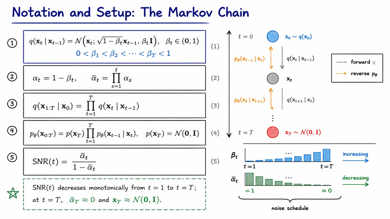
The forward process is defined as a discrete-time Markov chain of length , operating on random variables . The data sample is drawn from the unknown data distribution . Each subsequent variable is produced by a single Gaussian step:
Every step does two things simultaneously: it shrinks the mean by a factor of and injects fresh Gaussian noise with variance . The shrinkage is essential — without it, the variance would grow without bound. With it, one can show that as the marginal converges to a standard normal, regardless of what looked like. The noise schedule is a design choice: early steps add little noise (preserving fine structure), while later steps destroy information aggressively. Typical schedules are linear, cosine, or learned.
To keep notation compact, define:
Think of as the signal retention factor at step : it is close to 1 when is small (early, low-noise steps) and falls toward 0 as noise accumulates. The cumulative product is the key quantity in the entire framework. It measures how much of the original signal survives after noising steps. When , the sample is nearly clean; when , the sample is nearly pure noise. We will see in the next section that lets us jump directly from to any without simulating every intermediate step — a property that is absolutely critical for efficient training.
Because the forward process is Markov, the joint forward distribution over the entire trajectory factors as a product of one-step kernels:
There are no parameters to learn here; is entirely fixed by the schedule . This is a crucial asymmetry: the forward process is a known, deterministic recipe, while the reverse process must be approximated.
The reverse generative process mirrors the Markov factorization but runs backwards and uses learned parameters :
Generation begins by sampling from a standard normal — cheap and parameter-free — and then iteratively applies learned denoising kernels to recover a sample that looks like it came from . In practice each is itself taken to be Gaussian, with a mean predicted by a neural network and a fixed or learned variance. The Gaussian assumption in the reverse process is not trivially justified — it holds approximately when each is small, because the true reverse posteriors are then nearly Gaussian. This is why small step sizes (large ) matter.
Finally, it is worth naming the signal-to-noise ratio now, even though it plays a starring role only in later derivations:
The SNR decreases monotonically from (where it is high, close to ) down to nearly zero at . This quantity reappears naturally when bounding the ELBO, when choosing loss weightings, and when comparing different noise schedules. The conceptual message is simple: tracks signal, tracks noise power, and their ratio summarizes the information content at each timestep.
The visual below consolidates the entire notational setup into a single reference diagram. On one side, the core equations are laid out in their logical order — the forward kernel, the definitions, the joint factorization, the reverse factorization, and the SNR — numbered so you can cross-reference them as derivations proceed. On the other side, a vertical timeline makes the Markov structure legible at a glance: (a structured data point) sits at the top, sits at the bottom, and the forward arrows () and dashed reverse arrows () run in opposite directions along the same chain. Below the chain, a simple bar chart illustrates the noise schedule: climbs monotonically while falls, converging to zero as the SNR bottoms out.
Together, the equations and the diagram make concrete what might otherwise feel like a tangle of subscripts: there are exactly two processes, one fixed and one learned, they share the same Markov graph, and the single number is the bridge that will let us derive everything that follows without ever simulating the chain step by step.
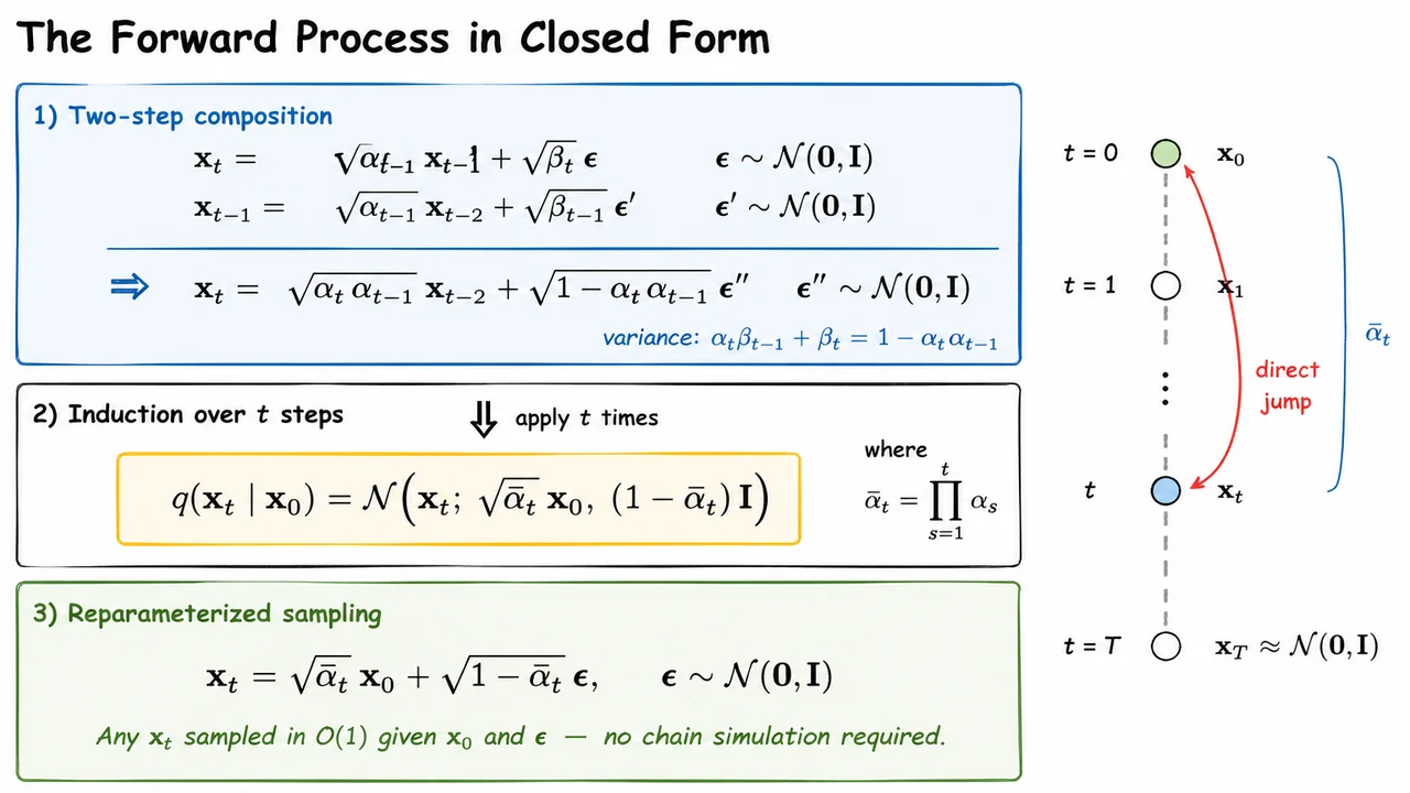
Having established the Markov chain structure of the forward process — where each step applies a small Gaussian perturbation to the previous sample — a natural and practically critical question arises: do we really need to simulate all steps of the chain every time we want to train the model? At first glance, computing from seems to require iterating through sequential transitions, which would make training prohibitively expensive for large . The key insight of DDPMs is that the Gaussian structure of the forward kernel makes this chain collapsible — we can jump directly from to any in a single step.
To see why, start from the one-step reparameterization implied by the Markov kernel , where we define . Writing this in reparameterized form:
Now unfold one additional step by substituting with an independent noise draw :
The two noise terms are independent Gaussians, so their sum is itself Gaussian with variance . The elegant algebraic fact is that this simplifies to , because . Folding the two noise terms into a single gives:
This is structurally identical to the one-step formula, with playing the role of the single-step . The pattern is unmistakable, and induction closes the argument immediately. Applying the same merging procedure times and defining the cumulative noise schedule , we arrive at the closed-form marginal:
or equivalently in the reparameterized sampling form:
It is worth pausing to appreciate the geometry encoded in this result. The noisy sample is a linear interpolation in variance space between the clean signal and pure isotropic noise: the coefficient scales the signal component, while scales the noise component, and the two squared coefficients sum exactly to one. As , and the distribution of collapses to — the data is fully destroyed. Near , and is nearly unchanged. The schedule (and hence ) controls how quickly this transition happens, with linear, cosine, and learned schedules each offering different tradeoffs in practice.
The practical consequence is profound. During training, we need to evaluate the model's denoising ability at a randomly chosen timestep for each mini-batch example. Without this closed form, that would require simulating the entire Markov chain from to , meaning sequential Gaussian samples. With the closed form, we instead draw , sample , compute , and immediately present the corrupted image to the network. The entire forward pass is regardless of , which is what makes DDPM training scalable to thousands of timesteps.
One subtle assumption underlying this derivation is the independence of noise draws at each step of the chain. Because we condition on the current state when sampling the next, the individual terms are independent by the Markov property — and it is exactly this independence that allows us to merge them into a single equivalent Gaussian. If the noise were correlated across steps (as in some non-Markovian variants explored later), the composition would not simplify so cleanly. This independence is not just a convenience; it is a structural prerequisite for the entire derivation.
The visual below distills this derivation into three logical layers that mirror the argument exactly. The top panel captures the two-step composition, showing how two sequential reparameterizations merge into one via the variance identity . The central panel presents the boxed main result — the closed-form marginal — highlighted to signal that this is the destination of the inductive argument. A small downward arrow labeled "apply times" bridges the two-step example to the general formula, making the inductive logic visually explicit.
The bottom panel reinforces the payoff: the reparameterized sampling equation and the consequence. A compact timeline diagram on the right margin shows the contrast most vividly — intermediate nodes are grayed out and bypassed, with a bold direct arrow leaping from to labeled by . That single arrow captures the entire point: a quantity that was seemingly chained across steps collapses, through the magic of Gaussian closure, into one line of arithmetic.
Having established that the forward process collapses any data point into near-isotropic Gaussian noise in closed form, the natural next question is: how do we train the reverse process at all? The marginal log-likelihood requires integrating over every possible noisy trajectory , which is combinatorially intractable. The classical remedy — borrowed straight from variational inference — is to construct a lower bound on that log-likelihood and maximize the bound instead.
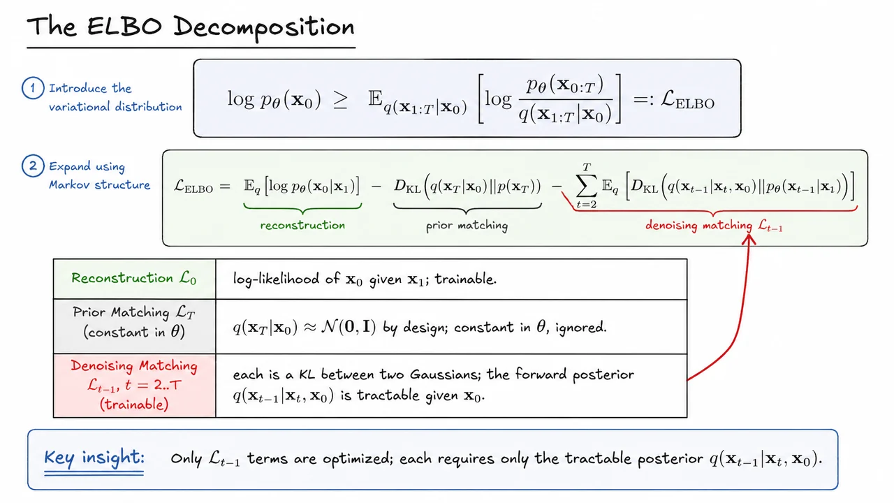
The variational lower bound (ELBO) arises by a single application of Jensen's inequality. Because is concave, we can multiply and divide the joint model density by the forward-process distribution and push the expectation outside the log:
This is identical in spirit to the VAE objective, with one crucial difference: the "encoder" here is the fixed forward diffusion process rather than a learned amortized network. That fixedness is both a gift and a constraint — it means we never have to worry about posterior collapse or encoder training instability, but it also means the variational gap is baked in by the noise schedule rather than being adaptively minimized.
The bound as written is still a monolithic expectation over all latents simultaneously. To make it actionable, we exploit the Markov structure of both the forward and reverse chains. Writing out the joint densities in terms of their conditional factors and canceling telescoping terms, the ELBO neatly separates into three semantically distinct pieces:
Each term has a distinct role, and understanding that role is the key to understanding why DDPMs are trainable at all.
The reconstruction term measures how well the learned reverse kernel recovers the original data from a lightly noised version. This is the only term that directly involves the data likelihood, and it is fully tractable to evaluate by sampling and evaluating the model's log-probability.
The prior-matching term penalizes any mismatch between the final noisy distribution and the standard Gaussian prior . Here is where the noise schedule design from the previous section pays off: by construction, , so regardless of . Consequently is essentially constant in and can be safely ignored during optimization. This is not an approximation we make for convenience — it is a design guarantee.
The denoising matching terms are where all the interesting training happens. Each one is a KL divergence between the reverse model kernel and the forward-process posterior . The latter, conditioning on both the current noisy state and the clean image, is a tractable Gaussian — a fact we will derive carefully in the next section. This tractability is the linchpin of the entire training algorithm: instead of asking "what is the reverse dynamics?", we ask "how closely does the model posterior match the Bayesian posterior conditioned on the data?" That question has an analytic, closed-form answer for Gaussian distributions, reducing each to a simple squared-distance between Gaussian parameters. The sum over then decomposes the training objective into independently optimizable terms, each targeting a single denoising step.
A subtle but important point: the conditional posterior is only tractable because we condition on . If we tried to compute without that conditioning, we would need to marginalize over all data points, which loops us back to the original intractability. The ELBO decomposition is clever precisely because it restructures the problem so that every term involves a quantity we can compute given a training sample .
It is also worth noting what this decomposition implies about the training loop. At each gradient step, we:
No simulation of the reverse chain is required during training. This is a critical practical advantage — in contrast to methods that must actually run the generative model forward to estimate gradients.
The visual below organizes this decomposition at a glance: the two key equations appear in shaded boxes, and below them a color-coded table separates the three terms by their gradient status. Green marks the reconstruction term (trainable), gray the prior-matching term (constant, ignored), and red the denoising terms (the main training targets). A callout arrow bridges the algebra in the second equation to the red row, making explicit that it is the sum — not the full ELBO monolith — that the optimizer actually touches. A blue box at the bottom crystallizes the key insight: the entire burden of learning falls on matching to a posterior we can compute exactly, one timestep at a time. Seeing the three rows laid out in isolation makes it immediately clear why the DDPM loss is so well-conditioned: the hard terms are constant, and the tractable terms each involve only a single Gaussian KL.
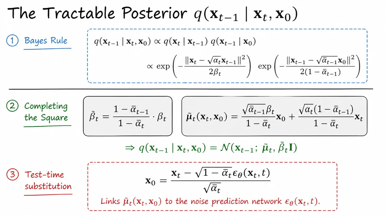
Having decomposed the ELBO into a sum of KL divergences, we face an immediate practical question: what exactly are we trying to match? Each KL term asks us to push the learned reverse distribution close to the true one-step backward conditional . The remarkable fact — one that makes DDPMs trainable at all — is that this backward conditional, while it would ordinarily be intractable, becomes an explicit Gaussian the moment we condition on the clean image . Let us derive this carefully.
The key move is Bayes' rule applied within the Markov structure of the forward process. Because the forward chain is Markov, we can write
The left-hand factor is the single-step transition, and the right-hand factor is the marginal obtained by running the forward process from for steps. Both of these are Gaussians we already have in closed form from the reparameterization of the forward process. Specifically,
Substituting these and taking the product of the two exponential kernels gives an unnormalized density in that is itself a Gaussian — but you have to complete the square to read off the parameters. Grouping the terms from both quadratics yields a precision (inverse variance) equal to
The posterior variance interpolates between (which would be the variance if we knew absolutely nothing about ) and something smaller, because the marginal provides additional information that sharpens the distribution. Notice that as , , so and the posterior collapses to a point — which makes perfect sense, because one diffusion step away from the clean image there is almost no uncertainty left given .
Reading off the mean of the completed square is equally illuminating. The posterior mean is
This is a convex-like weighted combination of the clean image and the noisy image . The weights are not arbitrary: the coefficient is large when is large (lots of noise was added at this step, so the clean image is very informative for denoising), while the coefficient is large when is large (we are far along the noising trajectory, so the current noisy state itself carries meaningful signal about where we were one step earlier). The two regimes blend smoothly across the whole diffusion timeline.
At this point the derivation is complete — but there is a crucial subtlety for test-time use. During training we have access to , so we can evaluate exactly. At inference, however, is the very thing we are trying to generate. Fortunately, the reparameterization trick from the forward process gives us an algebraic relationship:
where is the noise that was added to reach . At test time we replace with the network's prediction , giving an estimated . Substituting this estimate into the mean formula yields a fully computable reverse step — and, as we will see in the next section, this substitution also reveals why the ELBO collapses to a simple noise-prediction loss.
It is worth pausing to appreciate why this tractability is non-trivial. In a generic latent-variable model, the posterior would require integrating over complex non-linear transformations and would have no closed form. Here the entire chain is linear-Gaussian, which means Bayes' rule on products of Gaussians stays Gaussian. The DDPM design — using additive Gaussian noise with a variance schedule — is not just a convenient choice; it is the specific structure that makes the target distribution analytically tractable and therefore makes the KL in the ELBO computable without a variational approximation for .
The visual below consolidates this three-step derivation into a single structured layout. Starting from the Bayes' rule factorization at the top, the diagram traces the substitution of the forward Gaussians through the completing-the-square step, arriving at the two boxed results — and — as highlighted final quantities. A third block then shows the test-time substitution formula for in terms of the noise network, making explicit how the analytically derived mean connects to the trainable component of the model.
Seeing all three pieces together in this way clarifies the logical dependencies: the posterior variance depends only on the noise schedule and is fixed before training begins; the posterior mean depends on , which during training is observed and at inference is replaced by a neural prediction. That clean separation between fixed geometry and learned content is what gives DDPMs their elegant training objective.
With the tractable posterior firmly in hand, we are finally in a position to ask the most practical question in the whole DDPM framework: what exactly should a neural network be trained to do, and what loss function should we optimize? The derivation that follows is perhaps the most important result in the diffusion model literature — not because it is mathematically deep, but because it is surprisingly simple, and that simplicity turns out to be a design choice, not a derivation necessity.
Recall that the full ELBO for a DDPM decomposes into a sum of KL divergence terms, one for each denoising step . Each term measures how well the learned reverse conditional matches the true posterior . Because both distributions are Gaussian, each KL reduces to a mean-squared difference between their respective means — and after substituting the reparameterization of the forward process, those means can be written entirely in terms of the noise that was added. Specifically, the forward process satisfies the closed-form expression
which means that sampling a noisy image at any timestep is just a single, embarrassingly cheap operation — no sequential simulation needed. This is often called the reparameterization trick for the forward process, and it is what makes the following simplification tractable.
When you work through the algebra, each KL term in the ELBO becomes proportional to
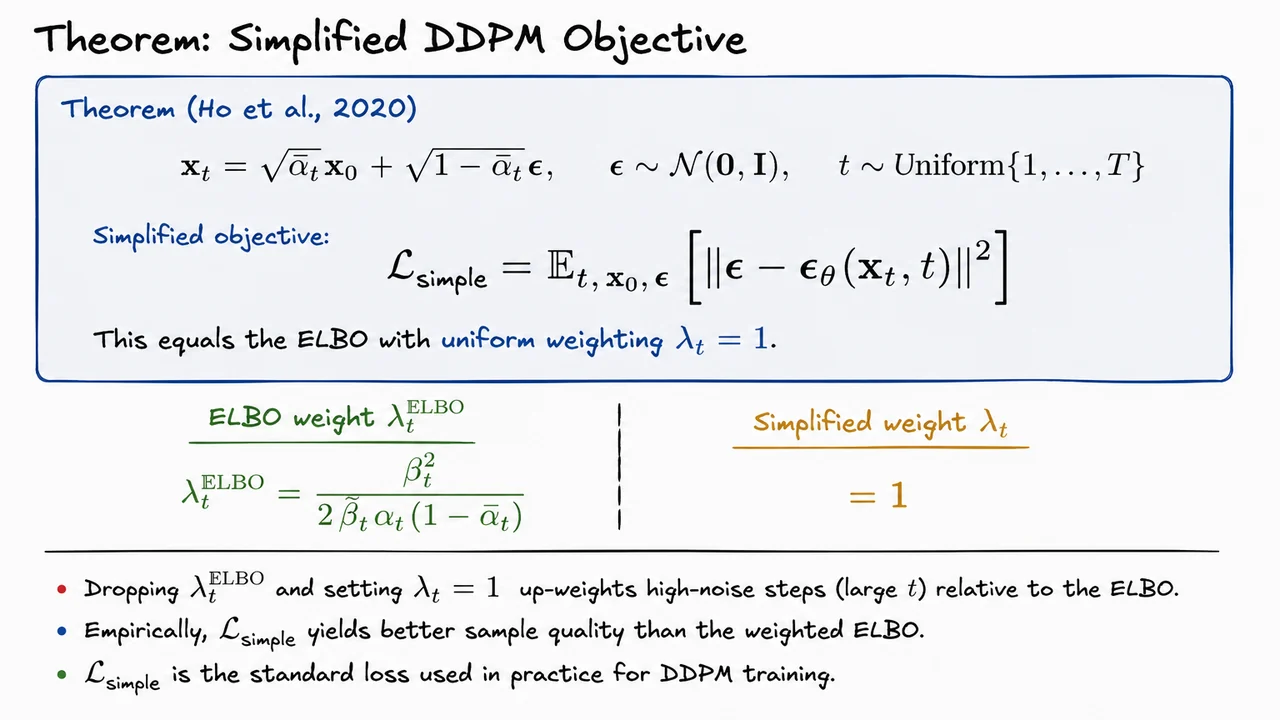
where the network is trained to predict the noise that was mixed into to produce . The ELBO weighting coefficient is
where is the posterior variance and . This is a complicated, timestep-dependent scalar. For small (low noise), is tiny and this weight is near zero, meaning the ELBO barely penalizes errors at easy, nearly-clean timesteps. For large (heavy noise), the weight grows but in a non-uniform way that is dictated purely by the noise schedule arithmetic.
Ho et al. (2020) made the empirically motivated decision to drop entirely and replace it with a constant weight of . The result is the simplified objective:
This is just an MSE loss on noise prediction, averaged uniformly over all timesteps, all data points, and all noise draws. The relationship to the ELBO is clean: is a reweighted version of the ELBO, with the theoretically correct weights replaced by uniform weights. The trade-off is illuminating:
Why should this up-weighting help? Intuitively, getting the coarse, high-noise denoising right has a large effect on the macroscopic structure of the generated image. The ELBO, which is derived as a lower bound on log-likelihood, cares most about the fine-grained steps where the distribution is concentrated near real data — but perceptual sample quality is governed by whether the model correctly captures the rough composition of a scene, which lives at high noise levels. The simplified objective implicitly acknowledges this by allocating equal training pressure across all noise scales.
There is a subtle but important subtlety worth pausing on: is not guaranteed to improve the marginal likelihood. It is a heuristic deviation from the ELBO, and in principle one could find settings where the weighted ELBO trains a model with higher likelihood. The empirical finding that the simplified loss produces better-looking samples tells us that DDPM training is not primarily about maximizing likelihood — it is about learning a good noise-to-image mapping across all scales. This philosophical point connects to the broader debate between likelihood-based objectives and perceptual quality in generative modeling.
Algorithmically, the training loop that follows from is remarkably clean: sample from data, sample uniformly, sample , construct in one shot, forward-pass through , and take a gradient step on the squared error. No simulation of the Markov chain is needed during training. This simulation-free property, inherited directly from the closed-form forward process, is one of the core reasons DDPMs are practical to train at scale.
The visual below consolidates exactly this comparison. At the top, the theorem statement anchors the derivation with the closed-form forward process and the MSE loss. The side-by-side comparison beneath it — the complicated fraction on the left versus the constant on the right — makes the design choice tangible: one weighting is what the math demands, and the other is what works in practice. This gap between theoretical optimality and empirical performance is a recurring theme in deep generative modeling, and seeing it laid out side by side makes the theorem feel less like a formal result and more like a principled engineering decision backed by evidence.
Having established the form of the ELBO and identified its dominant terms as KL divergences between consecutive-step distributions, the natural next question is: why does minimizing this complex variational bound reduce, in practice, to something as clean as predicting Gaussian noise with mean-squared error? The answer lies in a beautiful chain of substitutions, each one stripping away a layer of complexity until only the essential signal remains.
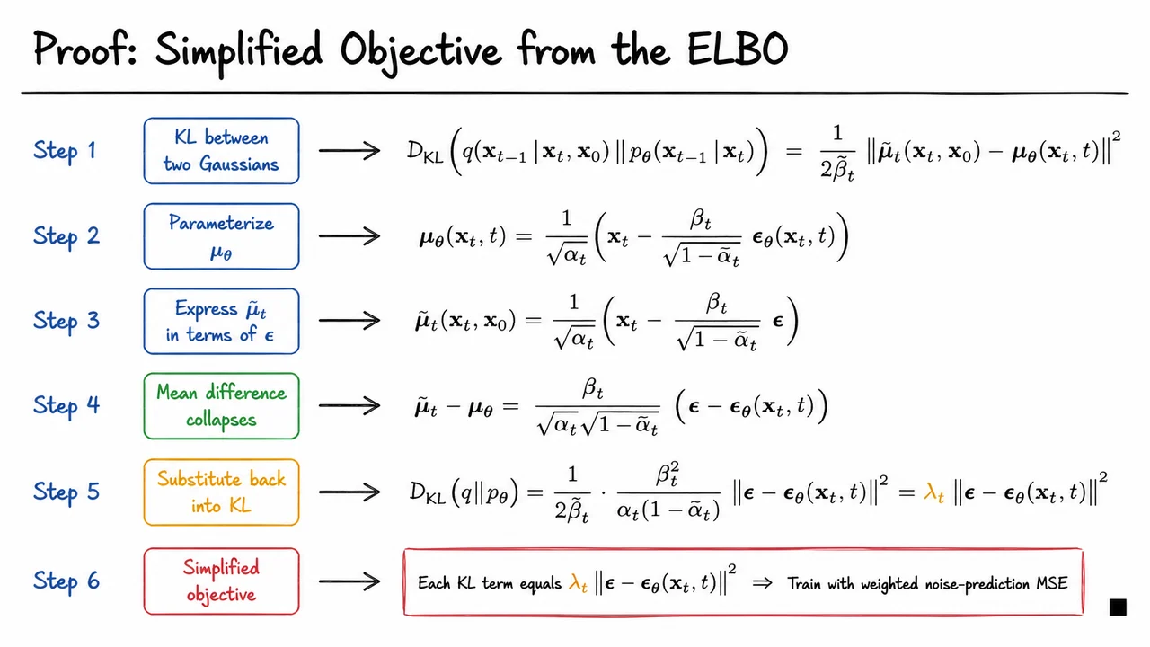
The first key observation is a standard fact about Gaussian distributions: the KL divergence between two Gaussians that share the same covariance depends only on their means. Concretely, if both and are , the general KL formula collapses entirely to a squared Euclidean distance between their means, scaled by the shared variance:
The design choice to fix the variance of the reverse process to the same schedule as the tractable posterior is therefore not cosmetic — it is what makes the objective analytically tractable. If the variances differed, the KL would carry additional log-determinant terms that would couple the variance and mean learning problems together.
The second move is to choose a specific parameterization of the learned mean . Rather than having the network directly predict the denoised mean, Ho et al. mirror the functional form of the true posterior mean , but replace the true noise with a neural network prediction :
This is a re-parameterization in the spirit of the reparameterization trick — instead of predicting a point in data space directly, the network predicts the noise that was mixed in during the forward process. The structural advantage is that already tells us the ground truth: the "correct" noise is exactly . Knowing this, we can also re-express the true posterior mean by inverting the forward process equation to write and substituting:
The structural symmetry here is striking: both and have identical scaffolding — the same prefactor , the same term, and the same coefficient — differing only in whether the noise slot is occupied by the true or the predicted . This means the difference of the two means collapses cleanly:
Substituting this into the KL expression, we get a weighted noise-prediction MSE at each timestep:
The full ELBO is a sum of such terms over , each carrying its own time-dependent weight . In principle, one could train with these exact weights, and some follow-up works explore the benefits of doing so. However, Ho et al. found empirically that dropping the weighting entirely — treating every timestep as equally important by setting and sampling uniformly — leads to better sample quality. The resulting objective is the celebrated simplified loss:
Why does dropping the weights work? Intuitively, down-weights timesteps near where the noise level is high and the signal-to-noise ratio is low — but those steps contribute substantially to perceptual quality. Equalizing the weights implicitly up-weights the high-noise regime, encouraging the model to learn coarse structure as well as fine detail, which turns out to be beneficial for image generation.
It is worth pausing on what makes this proof non-trivial. The whole reduction depends on three independently motivated design decisions clicking together: (1) matching the variances of the forward posterior and the reverse model, (2) parameterizing the reverse mean in the noise-prediction form, and (3) expressing the true posterior mean via the forward process reparameterization. Any one of these could have been done differently — and the ELBO would still be a valid bound — but only this combination produces the satisfying cancellation above.
The visual below traces exactly this chain of five algebraic steps, arranged as a vertical proof flow. Each step is annotated with the key substitution being made — from the KL simplification for equal-variance Gaussians, through the noise reparameterization, to the mean-difference collapse — culminating in the final weighted MSE and the simplified form with weights dropped. Seeing the steps in sequence makes viscerally clear how the structural symmetry between and is by construction, not by coincidence, and why the final objective is both correct and surprisingly simple.
Having worked through the ELBO and its simplification, we now arrive at the satisfying payoff: the full training and sampling procedures collapse into two clean, implementable loops. This is the moment where the theoretical machinery earns its keep — everything that looked complicated reduces to something a practitioner can actually run.
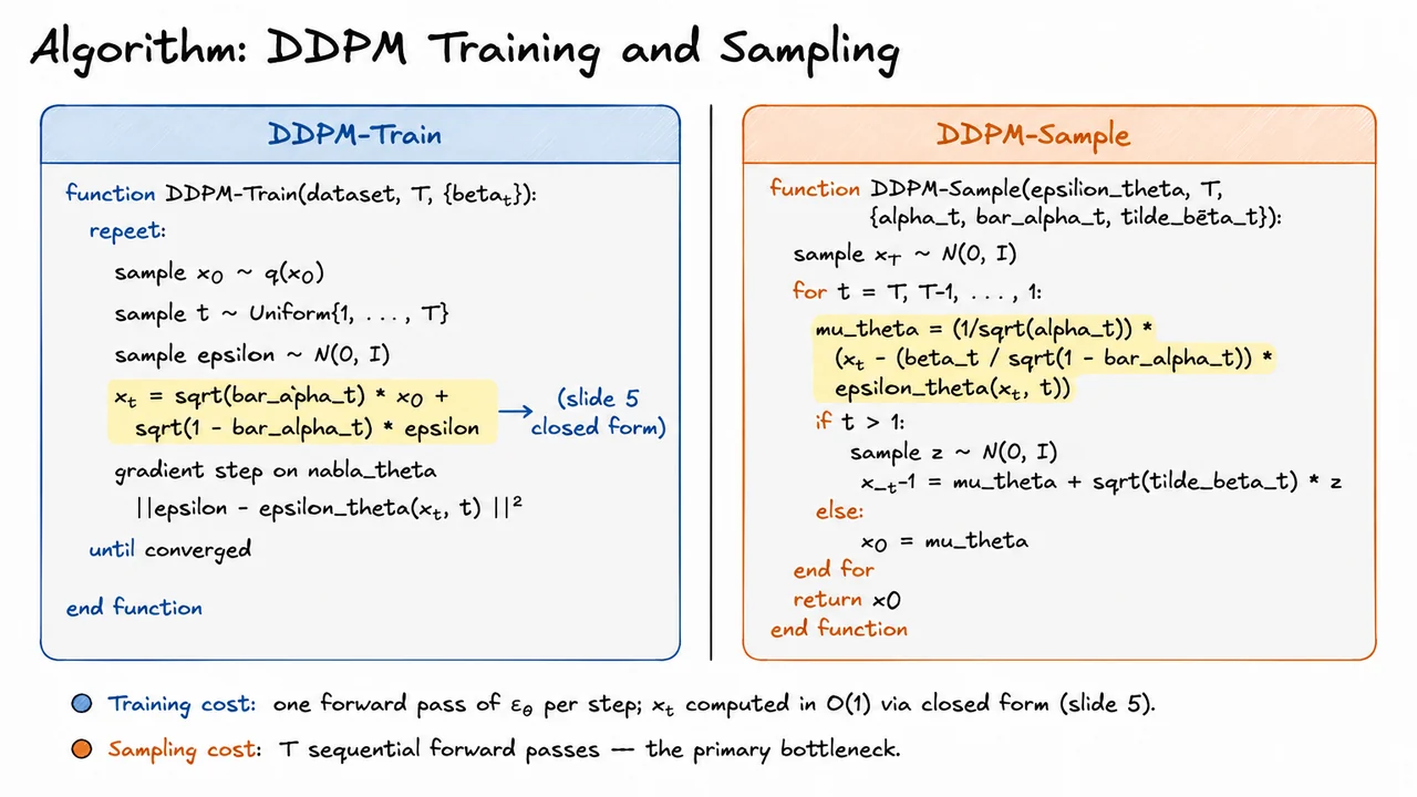
Training a DDPM is remarkably cheap per step. The key insight, established when we derived the reparameterized forward process, is that we never need to simulate the Markov chain one step at a time. Given a clean data sample , we can jump directly to any noise level in closed form:
where . This single equation replaces what would otherwise be sequential Gaussian corruptions. The cost is arithmetic regardless of how large is. Training therefore samples a random uniformly, constructs instantly, runs one forward pass of the noise-prediction network , and takes a gradient step on the simplified objective:
There are no KL divergences to compute explicitly, no importance weights, and no recurrence. Each training iteration is as cheap as a single supervised regression step, which is a large part of why DDPMs are tractable at scale.
Sampling, however, is a different story. To generate a new sample we must run the reverse Markov chain from pure noise all the way back to . At each step , the network predicts the noise component, which is used to reconstruct the posterior mean:
For , a small amount of Gaussian noise is added to this mean to sample the full posterior , preserving the stochastic character of the process. At the final step , no noise is added and is returned directly as .
This sequential structure is the primary computational bottleneck of diffusion models. Training needs exactly one network evaluation per gradient step. Sampling needs exactly network evaluations per generated sample, and crucially these evaluations are strictly sequential — each depends on the output of the previous step. With typical values of , generating a single image costs a thousand forward passes through a large U-Net. There is no parallelism available across timesteps during inference. This asymmetry — cheap training, expensive sampling — is not a flaw that was overlooked; it is a fundamental consequence of the probabilistic formulation, and motivating much of the subsequent literature on accelerated samplers (DDIM, DPM-Solver) and ultimately flow matching.
It is worth noting a subtle but important boundary condition in the sampling loop. The variance schedule term is the posterior variance, not directly. Recall that , which approaches zero as because . This is why the case naturally collapses to a deterministic step — adding noise at the very last denoising step would undo the clean output we just produced.
The visual below presents both algorithms side by side as annotated pseudocode. The training loop (left) draws attention to the single highlighted line where is computed in closed form — visually reinforcing that this is the entire "forward process" cost per step. The sampling loop (right) makes the sequential dependency explicit through its for-loop structure, with the computation highlighted to show where the network call sits inside every iteration. The contrast in loop structure between the two boxes captures the asymmetry at a glance: training is a simple repeat-until with no ordering constraint among iterations, while sampling is a strictly ordered for loop that cannot be vectorized across .
Together, the two boxes crystallize the engineering reality of DDPMs: if you need to train, the algorithm is as simple as noise regression can be; if you need to sample at scale, you will spend your compute budget in the reverse loop, and reducing that cost becomes the central engineering challenge.
Having walked through the DDPM training and sampling algorithm in the abstract, it is instructive to anchor all of those moving parts in a concrete, low-dimensional example where every number can be computed by hand. A one-dimensional bimodal distribution is the ideal stress-test: it is simple enough to reason about analytically, yet rich enough to expose the core tension in diffusion models — namely, whether the reverse process can faithfully recover multiple modes after the forward process has blurred them together into something that looks almost Gaussian.
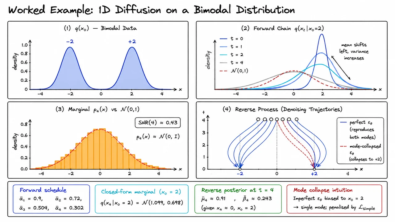
Let the data distribution be the equal-weight mixture
two narrow peaks sitting symmetrically at . We run a short forward chain of steps with a linearly growing noise schedule , giving . The cumulative signal-retention products are
These numbers tell a clean story. After just one step the signal retains 90% of its amplitude; by step 4 barely 30% survives. The closed-form marginal from the earlier reparametrisation says that, conditional on ,
The mean has drifted from all the way down to roughly , and the variance has ballooned to . Meanwhile the symmetric mode at produces a marginal centered near . When we mix across both modes, the marginal is the average of two broad, overlapping Gaussians that nearly cancel each other's asymmetry, producing something very close to . The signal-to-noise ratio at is
meaning there is less than half a unit of signal power for every unit of noise. Four aggressive steps have essentially destroyed the bimodal fingerprint of the data.
Now consider the reverse posterior. Given a noisy observation (which is right in the no-man's-land between the two modes) and conditioning on the true clean sample , the optimal one-step reverse mean is
with posterior variance . The first term pulls the estimate toward the clean signal , weighted by how much signal was already mixed in. The second term anchors the estimate in the noisy observation. This is the reverse process carefully triangulating its best guess of where should sit, given both the noisy present and the true past. Of course, at test time is unknown — the network must predict the noise that was added, from which the model implicitly reconstructs and therefore .
This is where mode collapse becomes a concrete, measurable failure. Because the data distribution is perfectly symmetric, an optimal must, on any given denoising step starting from , assign equal probability mass to paths leading toward and paths leading toward . A biased predictor — one that, say, always predicts noise consistent with — will incur a large MSE precisely in the half of training samples that came from the mode at . The simple denoising loss provides no escape hatch: every training example from the neglected mode directly penalises the collapsed prediction. Mode collapse is not a free lunch; it has a guaranteed, irreducible cost in training loss.
A few key takeaways crystallize from this worked example:
The visual below captures all four stages of this story at once. The top-left panel shows the pristine bimodal with its twin peaks. Moving to the top-right, you can watch the forward conditional evolve across : the mean slides left and the envelope broadens until the curve is barely distinguishable from the reference drawn in dashed red. The bottom-left panel shows sampled draws from against that same reference Gaussian, annotated with the computed SNR, making the near-total signal erasure visceral rather than abstract.
The bottom-right panel is perhaps the most instructive. It shows reverse-process trajectories fanning outward from back to . The blue trajectories from a perfect denoiser split symmetrically: roughly half arrive at and half at , faithfully mirroring the 50/50 prior. The red dashed trajectories from a mode-collapsed denoiser all converge on , visually dramatising exactly the failure mode that the MSE loss is designed to prevent. Together, the four panels compress the entire worked example — forward schedule, signal attenuation, reverse triangulation, and mode-collapse penalty — into a single, scannable figure.
Having established the closed-form marginal , a natural question emerges: how exactly should be chosen to decay from 1 to 0 over the steps? Everything about the training dynamics — the difficulty of the denoising task at each timestep, the faithfulness of the terminal distribution to a standard Gaussian, and the overall stability of the loss — hinges on this single scalar function of time. This is what a noise schedule controls.
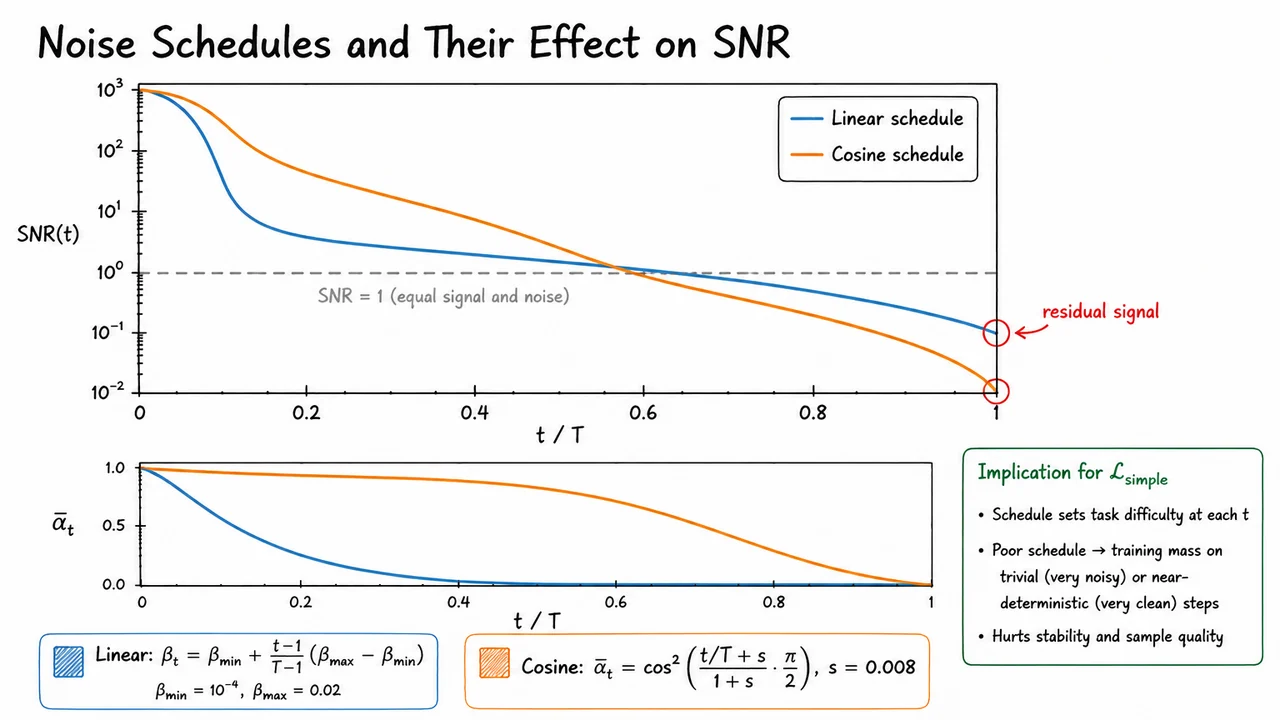
The most transparent lens through which to judge a schedule is the signal-to-noise ratio, defined at each timestep as
When , the data signal dominates and the noisy sample is almost identical to ; predicting the noise is nearly trivial. When , the signal has been completely swamped and looks like pure Gaussian noise; the prediction target becomes nearly meaningless. The ideal schedule should steer SNR on a smooth, controlled descent so that training effort is spread across genuinely informative, intermediate-difficulty timesteps.
The linear schedule, introduced by Ho et al. (2020), defines the per-step variance increments directly:
The cumulative signal retention is then , which decays roughly exponentially. The problem is subtle but consequential: because the values are small at early steps and grow only linearly to 0.02, the product does not quite reach zero, even at . Residual signal remains in , meaning the terminal distribution is not a clean standard Gaussian. This violates the prior assumption the reverse process is built on. At higher image resolutions the effect is even more pronounced, because the schedule was designed for 32×32 pixels and does not automatically compensate when the signal dimensionality grows.
The cosine schedule, proposed by Nichol & Dhariwal (2021), sidesteps the issue by parameterising directly rather than through individual :
The small offset prevents from being exactly 1 (which would cause numerical issues as SNR diverges) and ensures the schedule is well-behaved near . More importantly, the cosine function is chosen so that essentially by construction — the argument reaches at , and . The resulting SNR curve descends in a smooth S-shape on a logarithmic scale, spending more steps in the informative middle range where prediction is neither trivially easy nor hopelessly hard.
The practical consequence for training can be understood through the simplified objective . When timesteps are sampled uniformly and the schedule is poorly chosen, many sampled values will land in regions where the task is near-trivial — either the image is barely corrupted or it is already indistinguishable from noise — and gradient signal is weak. A well-calibrated schedule acts like an implicit curriculum: the model sees a balanced mixture of tasks ranging from fine-grained local denoising to coarse global structure recovery.
There is a deeper mathematical reason why SNR is the right summary statistic. One can show that the optimal denoising loss at any is a monotone function of alone, regardless of the specific path taken. Two schedules that share the same SNR curve are, in a precise sense, equivalent from the perspective of the learned score function, even if their individual sequences look different. This motivates treating SNR(t) as the primary object of study when comparing or designing schedules.
A few summary contrasts are worth keeping in mind:
The visual below consolidates everything just discussed into a comparative plot. The two SNR curves are shown on a logarithmic vertical axis — the natural scale for SNR, which spans several orders of magnitude — against normalised time . The blue linear-schedule curve drops steeply in the first 20% of the process and then flattens, arriving at with a non-trivial residual SNR, marked explicitly with a red circle labeled "residual signal." The orange cosine-schedule curve follows a smooth, nearly straight decline on the log scale and reaches SNR cleanly at . The horizontal dashed line at — the crossover point where signal and noise are equal in power — helps the eye locate how much of the diffusion trajectory each schedule spends in the meaningful intermediate regime. A companion inset of on a linear scale makes the same point geometrically, showing the cosine curve's characteristic plateau near and graceful tail near , contrasted with the near-exponential plunge of the linear curve. Together these two panels give an immediate, quantitative justification for preferring the cosine schedule in practice.
Having established how the noise schedule shapes the signal-to-noise ratio across diffusion timesteps, the next natural question is: what mathematical object should a neural network actually learn in order to reverse this process? The answer turns out to be the score function — a gradient field that, once learned, tells us how to walk back from noise toward data. Understanding why this object matters, and why naively estimating it is intractable, is the conceptual heart of score-based generative modeling.
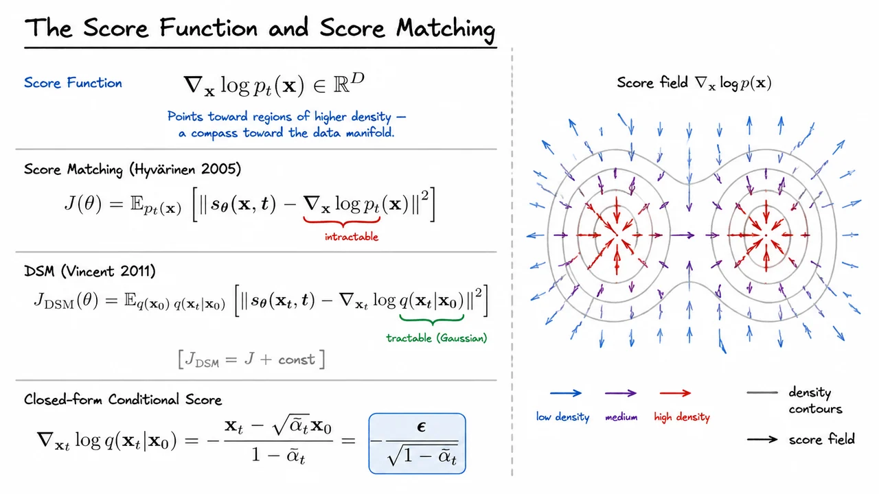
The score function of a probability density is simply its log-gradient with respect to the data variable:
Think of it geometrically: wherever the density is higher, the log-density is larger, so this gradient vector points uphill along the density landscape — toward regions of higher probability mass. It is a compass orienting us toward the data manifold, and crucially, it is defined everywhere in , not just where training samples happen to lie. This is quite different from a normalized density, which requires knowing the partition function. The score sidesteps that normalization entirely.
The natural training objective, proposed by Hyvärinen in 2005, is score matching: find a neural network that minimizes the expected squared deviation from the true score field,
This is a perfectly well-posed regression objective in principle. The problem, however, is immediate and severe: evaluating requires knowledge of the marginal distribution , which is the very thing we are trying to learn. For complex data distributions, this marginal is an intractable integral over all possible clean images. We cannot compute the target of our own regression.
This is where denoising score matching (DSM), introduced by Vincent in 2011, provides an elegant escape. The key insight is that instead of regressing onto the marginal score, we can regress onto the conditional score — the score of rather than . The DSM objective is:
Why is this valid? A short algebraic argument shows that expanding the squared norm in and integrating by parts (or equivalently, using the law of total expectation over the joint ) reveals that , where the constant does not depend on . The two objectives therefore share exactly the same minimizer. We have replaced an intractable target with a tractable one without any loss.
The tractability of the conditional score is not incidental — it follows directly from the Gaussian structure of the forward process. Recall from the forward noising derivation that . For any Gaussian, the log-density is a quadratic, and its gradient with respect to is simply the negative of the standardized residual:
where is the noise that was added during the forward pass. This final equality is a compact but powerful statement: the conditional score is exactly the injected noise, rescaled. The network does not need to estimate some abstract log-gradient — it needs to predict the noise that corrupted a clean image.
Several subtle points deserve emphasis. First, the equality holds because the conditional score is an unbiased estimator of the marginal score in the following precise sense: . The variance introduced by this substitution appears as the additive constant, which is irreducible and does not affect optimization. Second, the rescaling by means the magnitude of the score target grows as (low noise), which has practical implications for training stability and loss weighting — a theme we will revisit when connecting this to the DDPM noise-prediction objective.
The visual below captures this two-part story in a single glance. On one side, contour lines of a bimodal density are overlaid with arrows representing the score field — vectors pointing inward toward the two modes, with magnitude growing as you approach the high-density peaks. This makes viscerally concrete why the score is a "compass toward the data manifold." On the other side, the chain of equations is laid out with deliberate annotation: the marginal score is flagged as intractable, the conditional Gaussian score is flagged as tractable, and the closed-form expression is highlighted, emphasizing that the entire score-matching machinery ultimately reduces to predicting the injected noise. Together, the two halves of the diagram reflect the same intellectual journey we just traveled — from geometric intuition to computational necessity to closed-form resolution.
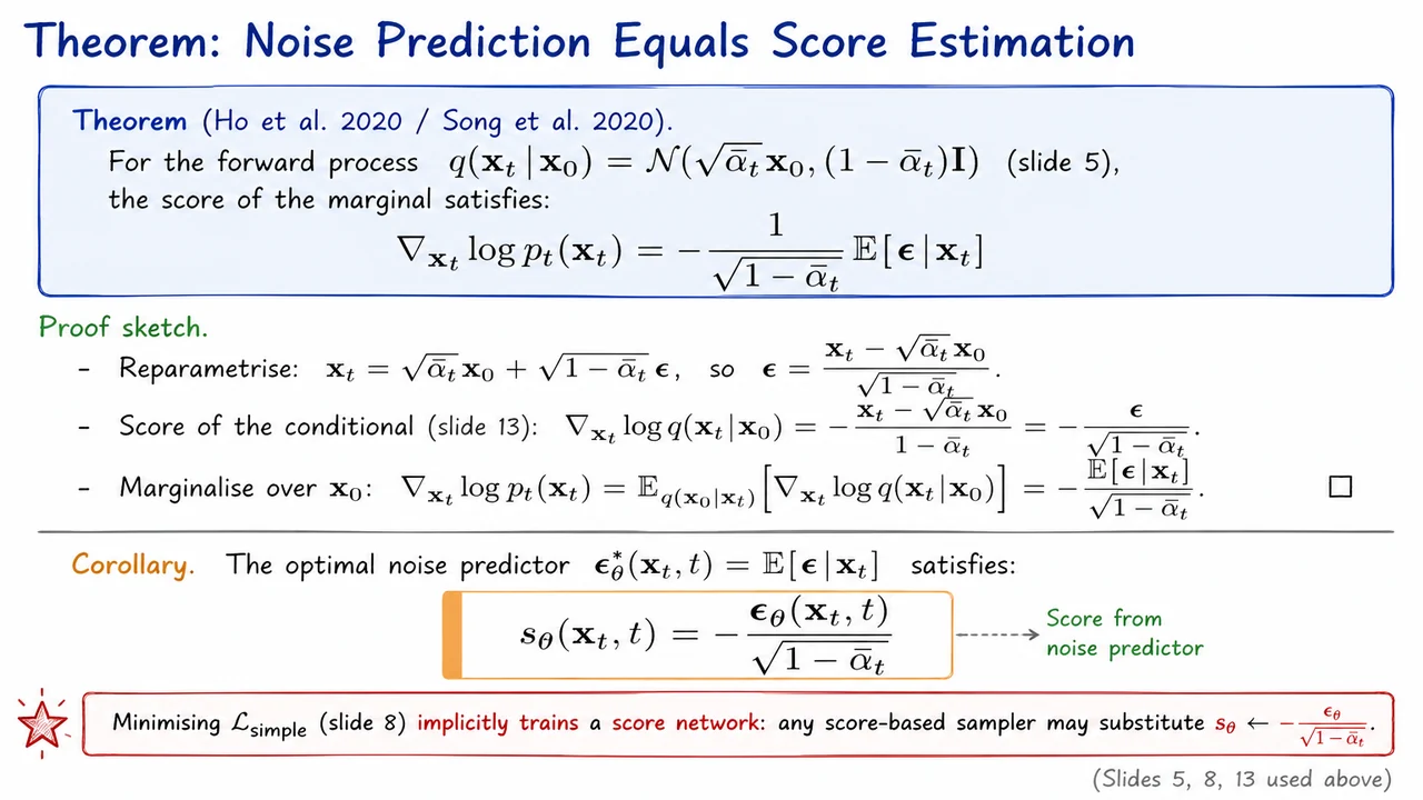
Having established that the score function is the central quantity driving any score-based sampler, a natural question arises: what is the DDPM noise network actually learning? The answer, formalized by Ho et al. (2020) and Song et al. (2020) independently, is one of the most elegant unification results in modern generative modeling — the noise predictor is the score function, up to a scalar factor that depends only on the noise schedule.
To see why, recall the DDPM reparametrization. The forward process at time is a single Gaussian,
which we can write in sample form as with . This is purely a change of variables. Crucially, because the conditional distribution is Gaussian, its log-gradient with respect to is just the negative scaled residual:
This step is worth pausing on. The noise is not an arbitrary training target chosen by practitioners for numerical convenience — it is literally the score of the conditional distribution, rescaled by . The variance in the denominator is precisely what converts the Gaussian residual into a log-gradient.
Now, to obtain the score of the marginal — the distribution that a score-based sampler actually needs — we must integrate out the unknown clean image . This is where Tweedie's identity and a key identity for log-gradients come together. Because the score of a mixture is a posterior-weighted average of the component scores,
Substituting the conditional score derived above, the expectation passes through the fixed rescaling factor:
This is the theorem. The marginal score equals the posterior mean noise divided by , with a minus sign. There is no approximation here — the equality is exact, contingent only on the Gaussian form of the forward process.
Why does this matter so much? The DDPM training objective minimizes , which by the law of total expectation pushes at optimality. Combined with the theorem, the corollary is immediate:
This single identity bridges two entire research programs. A network trained with the simple denoising MSE loss can be plugged directly into any score-based sampler — Langevin dynamics, the probability flow ODE, or any SDE solver from Song et al.'s framework — simply by substituting . Conversely, a score network trained via denoising score matching is implicitly a noise predictor. The two paradigms are not competing; they are the same parametric family wearing different hats.
A subtle but important assumption lurking here is that the marginal score identity holds only because the conditional distribution is Gaussian and the marginalization is over a continuous latent . If the forward process were non-Gaussian — as in discrete-state or categorical diffusion — the identity breaks, and noise prediction and score matching are no longer interchangeable. The Gaussian structure of the variance-preserving SDE is load-bearing.
The visual below captures the logical skeleton of this result in one frame. On one side sits the DDPM objective, minimizing against the concrete noise sample; on the other side sits the score network , the object score-based samplers demand. A single arrow, labeled with the scalar , connects them, and the central equation anchoring the diagram is the corollary itself. The proof steps appear as a compact derivation chain above: reparametrize, differentiate the Gaussian log-density, then marginalize by swapping expectation and gradient.
Reading the diagram after working through the algebra, one sees why this is considered a "free lunch" in diffusion research. There is no additional training cost, no architectural change, and no hyperparameter to tune. The rescaling is a closed-form function of the noise schedule , known at every timestep. The practical takeaway — that any well-trained DDPM is already a score model — has been exploited in virtually every subsequent sampler design, from DDIM to DPM-Solver to the continuous-time SDE framework, and it is the reason the field converged so rapidly on a unified theoretical language.
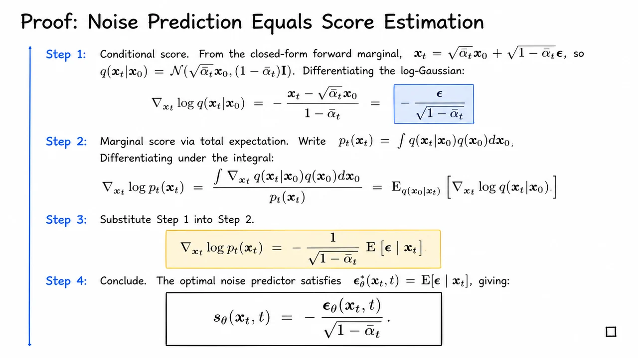
Building on the theorem we just stated — that training a DDPM noise predictor is secretly equivalent to learning the score function — we now carry out the proof explicitly. The argument is refreshingly clean: it requires nothing beyond differentiating a Gaussian log-density, exchanging a derivative with an integral, and applying the law of total expectation. Each step earns its place, and together they reveal exactly why the two objectives are related by a simple scalar rescaling rather than by some complicated functional transformation.
Step 1: The conditional score is just the scaled noise. Recall the closed-form forward marginal derived earlier:
This tells us that, conditioned on , the noisy sample follows a Gaussian with mean and variance . Differentiating the log of that Gaussian with respect to is completely mechanical — the log-normalizer vanishes and the quadratic gives a linear residual:
Now substitute the reparameterization: . The in the denominator cancels one factor of , leaving:
This is the key algebraic insight: the score of the conditional distribution is exactly the noise , rescaled by the standard deviation of the forward kernel.
Step 2: Moving from conditional to marginal via differentiation under the integral. The marginal density at time is the mixture . To get its score, we take the gradient of its log. A standard identity lets us push the gradient inside the integral — valid here because the Gaussian kernel is smooth and appropriately dominated — and then pull a back out:
Recognising and using Bayes' theorem to identify , the whole expression collapses to a posterior expectation:
This is the law of total expectation applied to the score: the marginal score equals the expected conditional score under the posterior over clean data.
Step 3: Combining the results. Substituting the expression from Step 1 into the expectation from Step 2 is trivial because the rescaling factor does not depend on and slides outside the expectation:
The marginal score is therefore proportional to the posterior mean of the noise given the observed noisy sample. This is a profound statement: despite the fact that we cannot compute the marginal explicitly, its score can be expressed as a conditional expectation that a neural network can learn to approximate.
Step 4: The final identification. When we train a DDPM, the optimal noise predictor in the sense satisfies — it is exactly the posterior mean of the noise. Plugging this into Step 3 gives the central result:
The score network and the noise-prediction network are thus the same network, just dressed differently. Converting one into the other requires only a scalar division by . This equivalence is not an approximation — it is exact at the level of optimal predictors. In practice, using a noise-parameterized objective rather than directly regressing the score leads to better-conditioned gradients, which partly explains DDPM's empirical success over earlier direct score-matching implementations.
It is also worth pausing on the subtle assumption embedded in Step 2: the exchange of differentiation and integration requires the integrand to be dominated by an integrable function uniformly in . Because is Gaussian and is a proper data distribution, this holds under mild moment conditions on the data — a regularity assumption that is almost always satisfied in practice but is worth keeping in mind if one ever considers heavy-tailed data distributions.
The visual below arranges these four steps in a compact proof layout, with the conditional-score equation highlighted in Step 1, the total-expectation derivation bridging Steps 1 and 2, the simplified marginal score in Step 3, and the final boxed identity in Step 4. Reading it top to bottom mirrors the logical chain: differentiate a Gaussian, push the gradient through the marginalizing integral, factor out the constant rescaling, and identify the posterior mean with the optimal network output. The thin vertical rule running along the left margin visually signals that all four steps form a single coherent argument, not independent claims.
Having shown that the noise-prediction network is, up to a rescaling, directly estimating the score , it is natural to ask what happens as the number of discrete diffusion steps grows without bound. The answer is elegant: the entire DDPM Markov chain converges to a stochastic differential equation, and the machinery of continuous-time stochastic calculus takes over. This shift from a discrete chain to a continuous-time SDE is not merely a mathematical formality — it unlocks a much richer theoretical toolkit and reveals a surprisingly clean connection between diffusion, density evolution, and deterministic sampling.
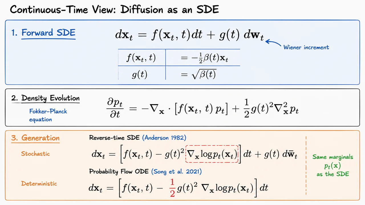
The forward SDE is the continuous limit of the repeated Gaussian transitions. As the step size shrinks and the number of steps , the discrete recurrence becomes an Itô stochastic differential equation:
where is a standard Wiener increment — the infinitesimal version of injecting Gaussian noise. For the variance-preserving schedule used in DDPM, the drift and diffusion coefficients take particularly simple forms:
The drift term gently shrinks the signal toward zero, while the diffusion coefficient injects noise at the same rate. Together they conspire to send any initial data distribution smoothly toward a standard Gaussian as .
How does the density evolve under this SDE? The answer is given by the Fokker–Planck equation, which can be derived by applying Itô's lemma to the SDE and reasoning about the probability flux:
The first term on the right is a transport term: it says that the drift field advects probability mass, just as a vector field advects fluid. The second term is a diffusion term: the noise causes probability mass to spread out, governed by the Laplacian. These two competing effects — compression via drift and spreading via noise — are precisely what keeps the process well-behaved. One subtle but important point is that this PDE holds for the marginal densities , not for individual sample paths. The Fokker–Planck equation is the deterministic law governing the evolution of the distribution, even though individual trajectories are stochastic.
Now comes the key theoretical move. Brian Anderson (1982) proved that every Itô diffusion has a reverse-time SDE, i.e., one can run time backwards from to and the resulting process has the same family of marginal densities . The reverse-time SDE is:
where is a reverse-time Wiener increment. The structure is striking: the reverse drift is exactly the forward drift minus the score function , scaled by . This is not a coincidence or a numerical trick — it is an exact mathematical identity. The score function is precisely the extra information needed to reverse diffusion. Plugging in the trained approximation gives a fully operational generative SDE sampler: start from Gaussian noise, integrate the reverse SDE from to , and obtain a sample from approximately .
One of the most practically important extensions, due to Song et al. (2021), is the probability flow ODE. The key observation is that the stochastic term in the reverse SDE is not strictly necessary to match the marginal densities. By halving the score correction and dropping the Wiener noise entirely, one obtains a deterministic ODE:
which can be shown — again via the Fokker–Planck equation — to preserve the exact same marginals as both the forward SDE and the reverse SDE. The word deterministic here is profound: given a fixed initial point in Gaussian space, the ODE traces a unique trajectory to a data point. This means the model is an implicit continuous normalizing flow, enabling exact likelihood computation and smooth interpolations in latent space. The price paid is that numerical ODE solvers must be used carefully, but off-the-shelf adaptive solvers (Dormand–Prince, Runge–Kutta) work well in practice.
It is worth pausing to appreciate why all three objects — the forward SDE, the reverse SDE, and the probability flow ODE — coexist so cleanly. They are three different processes that share the same marginal distributions. This is the heart of score-based generative modeling in continuous time: the score function is the single universal ingredient that connects all three, and our trained network provides it for free.
The visual below captures this three-way structure in a compact equation layout. The forward SDE sits in a blue-tinted block at the top, with its drift and diffusion coefficients made explicit — the small annotation on reminds us that randomness enters exactly here. The Fokker–Planck PDE occupies the middle block, representing the deterministic law that governs how density flows even as individual trajectories are stochastic. At the bottom, the generation block shows both the reverse SDE and the probability flow ODE side by side, with the score term boxed and the decisive factor-of-one-half difference between them highlighted — a compact visual proof that determinism costs only half the score correction. Together the three blocks make it easy to see that the same score function threads through every equation, which is precisely what justifies using trained by denoising to drive all three sampling strategies.
Having established the continuous-time SDE perspective and the probability flow ODE in the previous section, it is time to ask the most grounding question an empiricist can ask: does any of this actually work? Theoretical elegance is valuable, but the proof of a generative model lives in the quality of its samples, and that quality is measured — imperfectly but consistently — by the Fréchet Inception Distance (FID). Lower FID means the distribution of generated images is closer, in the feature space of a pre-trained Inception network, to the distribution of real images. With that metric in hand, we can situate the diffusion family concretely against a decade of competing methods.
Before looking at numbers, it is worth recalling what DDPM is actually optimising at training time. As derived earlier, Ho et al. (2020) showed that the full ELBO collapses, under the reparameterisation of predicting the added noise , to a surprisingly clean objective:
This is a mean-squared denoising loss on noise residuals, evaluated at uniformly sampled timesteps. The elegance of this form obscures a subtlety: the linear noise schedule governing turns out to be load-bearing. Small changes to the schedule shift the signal-to-noise ratio profile across timesteps and can meaningfully change which parts of the trajectory the network is forced to learn well. Ho et al.'s original linear schedule worked surprisingly well on CIFAR-10, but later work — notably Nichol and Dhariwal's improved DDPM — showed that a cosine schedule allocates capacity more uniformly and matters significantly on higher-resolution datasets like ImageNet.
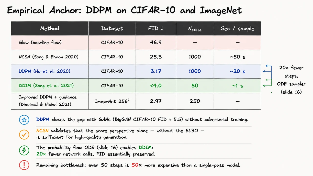
With a linear schedule and denoising steps, DDPM achieves FID 3.17 on CIFAR-10. To appreciate how remarkable that number is, consider the landscape it entered. Normalising flows like Glow, despite their elegant exact-likelihood training, produce FID scores around 46.9 on the same benchmark — more than an order of magnitude worse. The earlier score-based model NCSN (Song & Ermon 2020), which validated the score-matching perspective independently of the ELBO, improved this to 25.3 but still sat far from GANs. Meanwhile, BigGAN — the prevailing state-of-the-art GAN — achieved an FID of roughly 5.5 on CIFAR-10, and it required adversarial training with its attendant instability, mode-dropping risk, and architectural tricks. DDPM closed that gap and surpassed it, without a discriminator, without adversarial dynamics, using nothing more than a denoising regression loss and a U-Net backbone.
The result on ImageNet is equally striking. Dhariwal and Nichol (2021) extended the framework to resolution and introduced classifier guidance, which steers the reverse process using the gradient of a separately trained classifier's log-likelihood. This yields
at inference time, blending unconditional denoising with class-conditional gradient ascent. The result: FID 2.97 on ImageNet — decisively beating the GAN-based state of the art at the time.
Yet embedded in these triumphant numbers is an uncomfortable cost. Every one of those FID scores is purchased with a large number of sequential neural-network evaluations. DDPM on CIFAR-10 requires steps, taking roughly 20 seconds per sample on contemporaneous hardware. NCSN is even slower. This is not a minor inconvenience; it is a fundamental architectural tax. Each step involves a full forward pass of a U-Net, and the steps must be executed in sequence because each denoising step depends on the output of the previous one. There is no parallelism across the time axis.
Song et al. (2021) responded to this with DDIM (Denoising Diffusion Implicit Models), which reframes the reverse process not as a stochastic SDE but as a deterministic probability flow ODE — exactly the connection derived in the previous section. Because the ODE trajectory is deterministic, it can be traversed with larger step sizes using higher-order numerical integrators without the accumulated variance that makes large SDE steps unreliable. In practice, DDIM with only steps achieves FID below 4.0 on CIFAR-10 — a 20× reduction in network evaluations, with quality essentially preserved. Wall-clock time drops from roughly 20 seconds to roughly 1 second per sample.
That 20× speedup is impressive, but step back and consider the remaining gap. A single-pass generative model — a VAE decoder, a GAN generator, a normalising flow — produces a sample in one forward pass. Fifty steps is still fifty times more expensive. For high-resolution synthesis this translates to minutes per image rather than milliseconds. This arithmetic is not merely academic; it is the central engineering motivation for the next major paradigm shift in the lecture: flow matching. The question flow matching poses is simple and sharp — can we train a continuous normalising flow without simulation, reaching DDPM-level quality with a trajectory that can be traversed in far fewer steps, ideally approaching one?
The visual below consolidates these comparisons in one place. A comparison table lines up the five key methods — Glow, NCSN, DDPM, DDIM, and Improved DDPM with guidance — across dataset, FID, step count, and approximate sampling time. The DDPM row is highlighted to mark the breakthrough, the DDIM row to mark the efficiency gain, and an annotation arrow bridges the two with the label "20× fewer steps, ODE sampler." The Glow row serves as a stark baseline reminder that architectural choices in likelihood-based models matter enormously. Reading the table column by column, the story is clear: FID improves dramatically from Glow to DDPM, DDIM recovers that FID at a fraction of the step cost, and the remaining many-step burden across all rows sets the stage for why flow matching — with its simulation-free training and straighter trajectories — is worth studying carefully.
With the probability flow ODE firmly in hand from our study of score-based diffusion, it is natural to ask a liberating question: why should the drift be tied to any particular noising schedule at all? Diffusion models fix the forward process first and back out the reverse drift from the score function. But what if we simply wrote down a learnable ODE over and asked a neural network to discover the best possible transport on its own? That is exactly the premise of Continuous Normalizing Flows (CNFs), introduced by Chen et al. (2018), and it is a genuinely elegant idea whose power and whose pain are equally worth understanding.
A CNF defines a generative model through an autonomous ordinary differential equation,
where is any neural network — a U-Net, a transformer, anything. Integrating this ODE from to defines a flow map that pushes samples from the standard Gaussian forward into some distribution , which we hope approximates the data distribution . Unlike classical normalizing flows, which require architecturally constrained bijections (coupling layers, autoregressive maps) to keep the Jacobian determinant tractable, CNFs impose no structural constraint whatsoever on the network. Every design choice that makes normalizing flows brittle — invertibility by construction, triangular Jacobians, residual coupling blocks — simply vanishes.
The reason exact likelihoods are still available despite this freedom is the instantaneous change of variables formula. Because the flow is differentiable and the ODE is deterministic, the log-likelihood at time satisfies
This is a continuous-time analogue of the familiar log-determinant correction in discrete normalizing flows. The divergence tracks how much the vector field is locally expanding or contracting the volume element as probability mass flows through it. Accumulating this correction along the trajectory gives the exact log-likelihood — no variational bound, no KL divergence, no approximation of any kind. This is a theoretical achievement that diffusion models, relying on the ELBO, cannot match.
Yet this exactness carries a heavy price tag. Training by maximum likelihood estimation (MLE) requires evaluating the right-hand side of the log-likelihood equation for each training sample. That means two nested computational costs. First, you must simulate the ODE forward, which requires on the order of calls to the neural network — typically dozens to hundreds of evaluations depending on the solver tolerance. Second, at every single step of that solve, you must compute the divergence of . Because is a full neural network with no special structure, there is no closed-form divergence; instead one uses the Hutchinson trace estimator,
which requires at least one (and in practice several) Jacobian-vector products per step. Each Jacobian-vector product costs roughly as much as a single forward pass. So the total training cost scales as full network evaluations per training example, before even taking a gradient step.
Now consider the dimensionality of realistic image data. For a RGB image, the ambient dimension is . Each Jacobian-vector product traces through a high-dimensional network output; each ODE solve must be numerically stable across dozens of steps; and the entire computation must be differentiated through the ODE solver to backpropagate gradients into . The result is that naive MLE training of CNFs at image resolution is, bluntly, wall-clock intractable. Early CNF papers worked on toy two-dimensional distributions or tiny tabular datasets precisely because the scaling was so hostile.
This is the fundamental bottleneck that motivates everything that follows. CNFs are maximally expressive — any sufficiently powerful vector field can represent any diffeomorphism — and they offer exact likelihoods as a theoretical guarantee. But the ODE simulation requirement during training turns what should be a simple regression problem into an enormously expensive numerical integration problem. The crucial insight of flow matching, which we will develop in the next section, is that you can train to match a target vector field without ever simulating the ODE. Training becomes a simple supervised regression loss evaluated at randomly sampled times , with no ODE solver, no Hutchinson estimator, and no backpropagation through integration steps.
The visual below captures this two-sided story in a single glance. On the left, the CNF's generative mechanism is drawn as a clean transport: a Gaussian blob at is pushed rightward along smooth trajectories by the ODE drift, arriving at the data distribution at . The architecture-freedom and exact-likelihood properties sit on this side. On the right, the training bottleneck is laid out explicitly — the ODE solve, the divergence computation, and the frightening dimension count that makes each training step so expensive. A green box at the bottom of the right panel names the resolution: flow matching sidesteps the simulation entirely. This left-right contrast is not decorative; it is the logical structure of the argument. Understand both sides, and the motivation for flow matching becomes not just clear but inevitable.
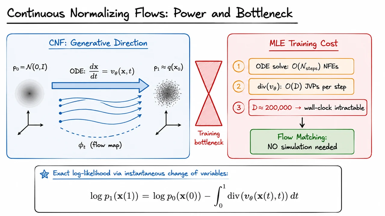
Having established that continuous normalizing flows are powerful but computationally expensive to train through simulation, we now arrive at the central question of flow matching: can we directly specify a target velocity field and regress onto it, entirely avoiding the ODE solver during training? The answer is yes — but it comes with a subtle and important intractability problem that shapes the entire framework.
The starting point is a probability path, a smoothly evolving family of distributions that interpolates between a simple source and a complex target. Concretely, we want:
At we begin with isotropic Gaussian noise — easy to sample. At we want to arrive at the data distribution — what we care about. Everything in between is a trajectory that some time-dependent velocity field must carve out. The goal of flow matching is to train a neural network to imitate this target field so that integrating the learned ODE at test time transports noise samples into realistic data.
The precise condition linking the velocity field to the evolving density is the continuity equation:
This is the statement that probability is conserved: the local rate of change of density equals the net flux of probability mass flowing in or out of each region. If you think of as a fluid density and as the velocity of that fluid, the continuity equation is simply the incompressible-flow conservation law lifted to probability space. Importantly, this is the deterministic counterpart of the Fokker–Planck equation we encountered earlier — there is no diffusion term, no noise injection, only pure transport. Every trajectory in this framework is a smooth deterministic path, which is one of the key geometric differences between flow matching and score-based diffusion.
Given a valid target field , the natural training objective is a simple mean-squared regression:
This is appealingly clean. Sample a time uniformly, sample a point from the marginal distribution at that time, and penalize the squared difference between the network's prediction and the true velocity at that point. Minimizing this objective should yield a network that, when integrated, traces out the probability path. The gradient of with respect to is unbiased and straightforward to compute — at least, in principle.
Here is the catch, and it is a serious one. Both the marginal density and the marginal vector field are defined by integrating over the entire data distribution:
The marginal at time is a mixture: for every possible data point , there is a conditional density describing where that data point's probability mass sits at time , and we average these over the data distribution. Similarly, the marginal velocity is a density-weighted average of conditional velocity fields. Unless the data distribution has a closed form — which it never does in practice — neither integral can be evaluated. You cannot sample from by marginalizing, you cannot evaluate pointwise, and therefore you cannot compute directly. The objective is well-defined as a mathematical object but computationally intractable.
This intractability is not a minor numerical inconvenience. It is a fundamental barrier: the target of the regression is an object you cannot access. One might hope to approximate the integral via Monte Carlo over , but that would introduce high variance and still require evaluating conditional velocities that may themselves be non-trivial. The right response — and the key insight of conditional flow matching — is to avoid computing the marginal entirely by reformulating the objective in terms of quantities conditioned on a single . The conditional path and the conditional velocity field are typically designed to have closed forms (for instance, simple Gaussian conditionals with linear interpolation). The remarkable fact, which we will derive in the next section, is that the Conditional Flow Matching (CFM) objective — which regresses onto these tractable conditional fields — shares identical gradients with . The intractable marginal target can be silently replaced by a tractable conditional one without changing the optimization landscape.
The visual below captures all three layers of this story in a single glance. On the right, a timeline runs from (Gaussian blob) to (irregular multimodal density), with intermediate marginals sketched in between and green arrows indicating the velocity field that would transport one to the next — this is the ideal picture, the thing we want. On the left, the three governing equations are laid out in order: boundary conditions, the continuity equation (highlighted as the structural constraint tying velocity to density), and the FM objective. The red intractability badge on the marginal densities is the visual punchline: everything in the right column is conceptually correct but practically out of reach, which is precisely why the conditional reformulation is necessary.
Together, the diagram makes it easy to internalize the two-step logic: first, there exists a clean velocity-regression objective that would work if we could evaluate marginals; second, we cannot evaluate those marginals, so a conditional surrogate is needed. That surrogate is the subject of the theorem we turn to next.
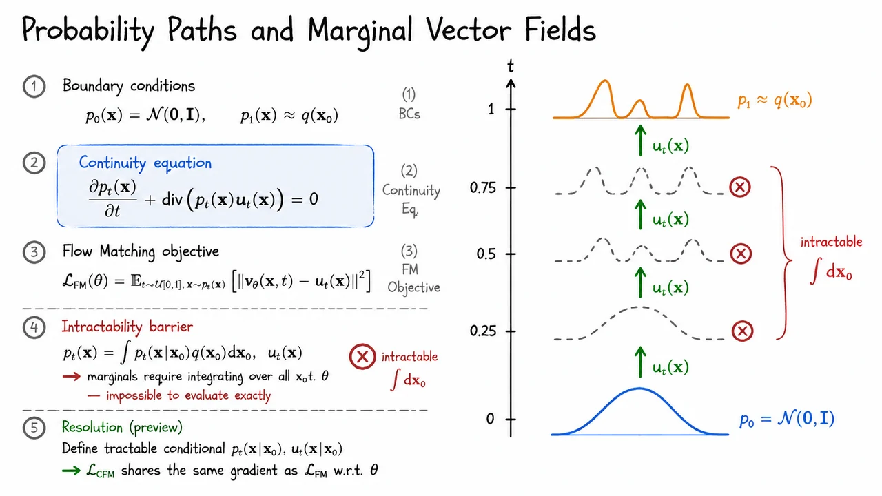
Having established that the marginal probability path and its generating vector field can both be written as weighted averages over conditional counterparts, we now face the central computational question: can we actually train a neural network to approximate without ever simulating an ODE? The Flow Matching objective says to regress directly onto , but itself requires integrating over all of data space — it is a marginal quantity that is every bit as intractable as the partition functions we spend so much effort avoiding elsewhere in generative modeling. The key theorem of Lipman et al. (2022) resolves this tension with elegant economy.
Recall the two marginal identities from the previous section. The marginal density is a mixture:
and the marginal vector field is a posterior-weighted average of conditional vector fields:
The conditional vector field is something we can freely design — for instance, a straight-line interpolation from a noise sample to . This is the handle we pull.
The intractable FM objective asks us to minimize
The problem is the expectation over and the evaluation of : both require the marginalization above. Sampling from forces us to first sample and then run the ODE forward, and computing at an arbitrary point involves that same intractable integral. Neither step admits a simple Monte Carlo estimator.
The Conditional Flow Matching (CFM) objective sidesteps both problems by conditioning before taking the expectation:
Every quantity in this expression is tractable by design. We sample a data point from the dataset, draw a time , then sample from the conditional — which, for Gaussian interpolants, is just a reparametrization trick. Finally, we evaluate in closed form from our chosen interpolation schedule. No ODE is touched.
The theorem's central claim is the gradient equivalence:
This is a stronger statement than the two objectives being equal up to a constant — it says that every gradient step taken on is a valid gradient step toward the minimizer of . The proof, which we will develop in the next section, proceeds by expanding both objectives and showing that the difference is a term that does not depend on , so it vanishes when differentiating. The key algebraic move involves recognizing that a cross-term proportional to integrates to zero via the law of iterated expectations and the tower property.
The practical consequence is profound. Training a continuous normalizing flow no longer requires adjoint-state ODE solvers, no backpropagation through a numerical integrator, and no expensive likelihood evaluations. The recipe collapses to three steps: sample , sample , evaluate the closed-form conditional target , and back-propagate through a mean-squared error. This is precisely the computational budget of training a vanilla denoising network in diffusion models, which is not a coincidence — denoising score matching is, in a meaningful sense, a special case of this framework.
It is worth pausing on why the gradient equivalence holds intuitively. The FM objective integrates over all of simultaneously, blending information from many data points into each gradient signal. The CFM objective decomposes that integral by conditioning on individual , trading a difficult marginal regression for many easier conditional regressions. Because the marginal vector field is a linear weighted combination of the conditional fields, the regression targets are consistent: the optimal conditional predictor aggregates to the optimal marginal predictor. It is the same logic that makes denoising autoencoders consistent estimators of the score — a conditional expectation, when averaged over the conditioning variable, recovers the marginal.
The visual below crystallizes the theorem's structure. A highlighted theorem box presents the three key equations in sequence — the marginal factorization, the CFM objective, and the gradient equality — with the gradient identity rendered prominently to signal that it is the load-bearing result. Below the box, the training algorithm reduces to three concise steps, each one tractable by construction, culminating in the emphatic conclusion that no ODE simulation is needed at training time. Seeing the three equations stacked together makes the logical progression clear: the first equation motivates why a conditional version of the problem exists, the second defines what we actually optimize, and the third tells us why doing so is legitimate.
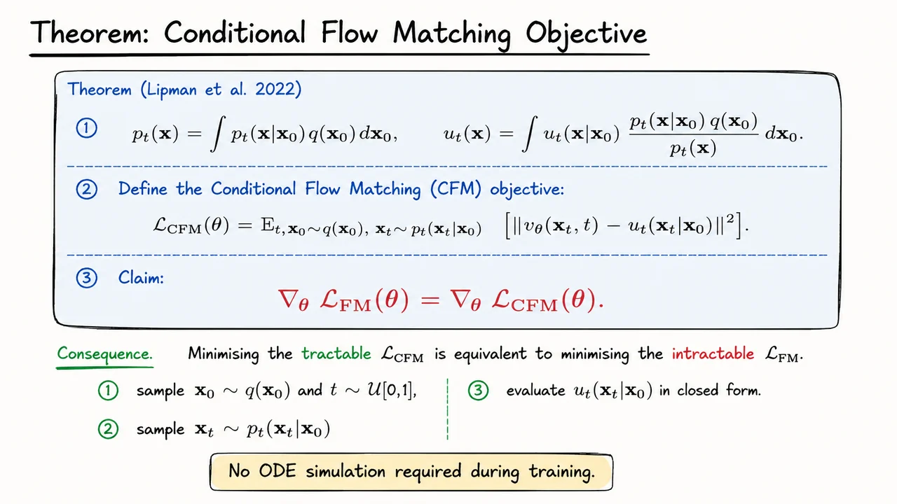
Having established the Conditional Flow Matching objective as a tractable surrogate, the natural question is whether we have actually preserved the optimization problem we care about. After all, replacing the marginal vector field with the conditional vector field is a substantial change in the regression target — it is far from obvious that a network trained under the conditional objective will converge to the same solution as one trained under the original FM objective. The proof that follows answers this question definitively: the two objectives differ by a constant that is entirely independent of the network parameters , so their gradients are identical everywhere.
Step 1: Expand the FM loss into three terms. The flow matching loss is a squared-norm regression objective, so expanding it quadratically is the natural first move:
The critical observation is immediate: term (C), the squared norm of the target vector field , does not contain at all. Only terms (A) and (B) drive the optimization. Term (C) is a constant shift that can be ignored for the purpose of finding the minimizer. The real work, therefore, lies in understanding what happens to the cross term (B).
Step 2: Rewrite the cross term using the marginal decomposition. The reason the FM objective is intractable in the first place is that is not available in closed form — it is defined as a weighted average of conditional vector fields over all possible data points:
When we substitute this definition into the expectation in term (B) and swap the order of integration — justified by Fubini's theorem under mild regularity conditions — a remarkable simplification occurs:
The outer expectation over the marginal paired with the marginal target is exactly equal to the outer expectation over the joint paired with the conditional target . This is the pivotal step: the cross term, which contains all of the -dependence beyond the squared network norm, is the same in both objectives.
Step 3: Expand the CFM loss and identify the match. Performing the identical quadratic expansion on the CFM objective,
we see that the -dependent terms — the squared network norm (A) and the cross term (B) — are identical to those in . The only structural difference between the two expanded losses is the final constant term: (C) uses the marginal target while CFM uses the conditional target .
Step 4: The difference is a constant, so gradients agree. Subtracting the two losses,
the right-hand side contains no whatsoever. Differentiating both sides with respect to immediately yields the central result:
This is a strikingly clean conclusion. The two norms on the right are not generally equal — the law of total variance implies that the marginal field has lower squared norm than the conditional field (averaging contracts magnitude), so the difference is typically negative. But that numerical gap is irrelevant for optimization: any gradient-based optimizer follows the same path regardless of which objective it is given, because they share the same loss landscape up to a vertical translation.
Why does this matter so much in practice? The FM objective involves integrating over the intractable marginal and evaluating the intractable vector field at each training step. Neither quantity can be sampled or computed without expensive simulation. The CFM objective, by contrast, requires only sampling a data point , constructing a noisy interpolant , and evaluating the analytically available conditional target . This proof guarantees that paying the lower computational price does not come with any optimization penalty.
The visual below encapsulates this four-step argument in a single compact layout. Each numbered step corresponds to one manipulation: the quadratic expansion with labeled (A), (B), (C) terms; the cross-term substitution that converts a marginal expectation into a joint one; the side-by-side alignment of CFM's expansion showing identical -dependent structure; and the final boxed conclusion isolating the constant difference and the gradient equality. Tracing through those four blocks in the diagram is the fastest way to reconstruct the proof from memory — and to appreciate that the entire argument hinges on one algebraic substitution, the swap of marginal for conditional that Fubini's theorem licenses freely.
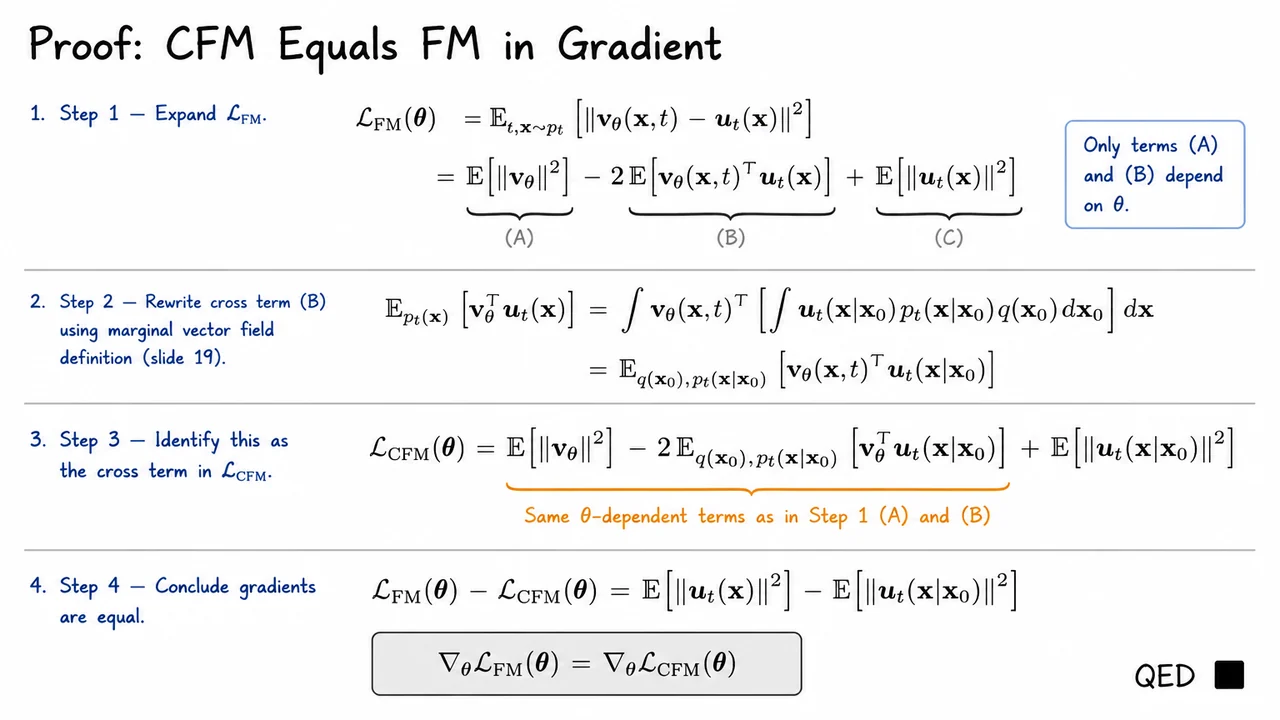
Having proved in the previous section that the gradient of the Conditional Flow Matching objective exactly equals the gradient of the intractable Flow Matching objective, we are now free to choose any conditional path we like — the training signal is guaranteed to be correct regardless. This freedom is the entire leverage point of CFM, and the question becomes: which conditional path makes the target vector field as simple as possible? The optimal-transport Gaussian path is the canonical answer, and it leads to something almost surprisingly clean.
The idea is to parameterize the conditional distribution as a Gaussian that interpolates between noise and data. Concretely, we set
and then choose the mean and standard deviation schedules according to the Optimal Transport (OT) interpolant of Lipman et al. (2022):
At the mean is zero and the standard deviation is one, so the marginal is pure Gaussian noise . At the mean is and the standard deviation has shrunk to the tiny constant , placing a tight Gaussian almost entirely on top of the data point. The interpolation is linear in both the mean and the standard deviation, which is the key structural choice.
To work with this path concretely, we use a reparameterization. Drawing independently, the sample at time is
This is just a convex-like combination of the noise and the target , with the noise weight shrinking linearly and the data weight growing linearly. The map is a flow map — it specifies where the particle starting at at time is located at any intermediate time.
The conditional vector field is now obtained by differentiating this flow map with respect to time:
Pause to appreciate what this says: the conditional vector field is constant in . It does not depend on the current position at all, only on the pair that defines the trajectory. Every particle travels in a straight line at uniform speed from to (approximately to when is small). This is the OT property: straight-line, constant-velocity displacement is the solution to the Brenier optimal transport problem between two Gaussians.
This observation directly determines the training loss. Since the conditional vector field is constant and closed-form, we can substitute it into the CFM objective to get a pure regression problem:
where the input to the network is the interpolated point and the regression target is a time-constant vector for each pair . There is no ODE simulation, no score network, no importance weighting — just a single forward pass to compute , then a squared-error penalty against a fixed vector. Compare this to diffusion-based training, where the score network must implicitly invert the forward process and the loss involves a carefully chosen weighting over noise levels. Flow matching with the OT path reduces to something closer to standard supervised regression.
It is worth noting a subtle but important assumption built into this choice: the noise that defines the starting point of a trajectory is paired independently with the data point . The resulting marginal paths can therefore cross in the ambient space — when viewed collectively across all pairs, different trajectories may intersect at intermediate times, even though each individual trajectory is straight. The marginal vector field is not itself a constant-velocity field; it is the average over all trajectories passing through at time , which can be curved. What is constant is the conditional field, and CFM trains precisely on this conditional target. The equivalence theorem from the previous section guarantees we still learn the correct marginal field.
The visual below makes this structure immediately legible. On the left, the derivation chain is laid out as a sequence of boxed equations, each following from the previous by differentiation or substitution — a compact proof that three lines of algebra suffice to go from the Gaussian path definition to a closed-form training target. On the right, the geometry comes alive: a set of straight-line trajectories depart from a diffuse Gaussian cloud at and arrive at structured data points at , with uniform tick marks along each line confirming constant speed. The tightening of the Gaussian width — from broad noise to a narrow bump around — corresponds to shrinking linearly. Taken together, the two halves of the diagram reflect exactly the two-sided simplicity of the OT interpolant: algebraically, the target is a time-constant closed-form vector; geometrically, the trajectories are straight lines traversed at uniform speed.
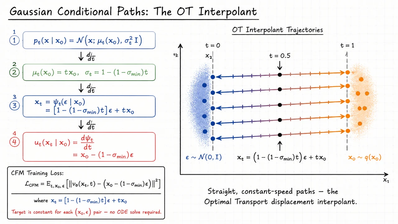
Having established the geometric structure of the OT conditional path, the natural next question is: what does the actual training loop look like in code, and how does sampling work once training is complete? The answer is striking in its simplicity — and that simplicity is precisely the point.
Recall where we left off. For a source noise sample and a data point , the OT interpolant traces a straight-line path between them:
Because this path is linear in , its time derivative — the conditional vector field that generates the flow — is constant throughout the trajectory. Differentiating with respect to :
This is a crucial observation. The target velocity does not depend on at all. For a fixed pair , the correct vector field is the same constant vector at every point along the straight-line path connecting them. This is what makes the flow matching loss so clean:
The network receives a noisy interpolant and a time index , and must predict a fixed, closed-form vector . There is no neural ODE rollout inside the training step, no likelihood computation, no expensive trace of a Jacobian — just a single forward pass followed by an MSE regression against an analytically known target.
This stands in sharp contrast to earlier continuous normalizing flow methods, where computing the change-of-variables likelihood required tracing the full ODE trajectory and estimating via Hutchinson's trick. That estimator is unbiased but noisy, and the ODE integration itself is computationally expensive, making every gradient step costly. Flow matching sidesteps both problems entirely. The simulation-free property is not a heuristic shortcut; it is an exact consequence of the conditional flow formulation and the fact that the marginal flow matching loss shares the same gradient as the intractable marginal objective.
The training algorithm is therefore a simple stochastic loop: sample a data point, sample noise, sample a time, form the interpolant, compute the target velocity, and take a gradient step. Each iteration touches the network exactly once. Convergence is stable because the regression target is deterministic given — there is no Monte Carlo variance introduced by ODE solvers or stochastic estimators. In practice, this translates to significantly faster wall-clock training compared to methods that must simulate trajectories.
Sampling is the reverse operation: starting from a fresh at , integrate the learned vector field forward to to produce a data sample. With step size , a simple Euler integrator reads:
Because the underlying trajectories are straight lines, the vector field is nearly constant along each path, which means Euler integration incurs very small discretization error even with a modest number of steps. This is one of the principal practical advantages of the OT interpolant over more curved trajectory families: the integrator does not need to chase a rapidly changing curvature, so the same sample quality is achievable with far fewer function evaluations. When higher-order accuracy is desired, the Euler step can be replaced by Heun's method, Runge–Kutta 4, or a specialized solver like DPM-Solver without changing the trained model at all — the choice of integrator is decoupled from the training objective.
A few subtleties are worth keeping in mind. The hyperparameter controls how much residual noise remains at relative to ; in the limit the path becomes an exact straight line from to . Small but nonzero (e.g., ) ensures the conditional distribution at is a narrow Gaussian centered on the data, which regularizes the vector field near the endpoints. The training loss is also not supervised in the traditional sense — we never observe the "true" marginal vector field; we only regress against conditional targets, and the equivalence of gradients between the conditional and marginal losses (proven in the flow matching theory) is the key theoretical guarantee that makes this work.
The visual below captures exactly this two-phase picture: a left panel showing the training loop as a concise pseudocode block — sample, interpolate, regress — and a right panel showing the Euler sampling loop. Accompanying annotations highlight the three properties that make the algorithm competitive: no ODE simulation at train time, a constant and analytically available regression target, and a solver-agnostic sampling procedure. Seeing both algorithms side by side makes it immediately apparent how much computational burden has been eliminated relative to earlier flow-based methods, and how naturally the clean geometry of straight-line paths translates into a clean, practical algorithm.
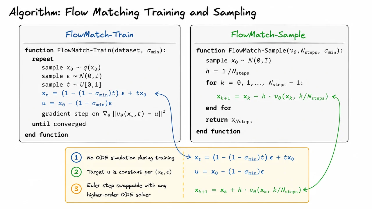
Having established the flow matching training loop — where a network learns to regress onto per-sample conditional vector fields and sampling proceeds by integrating the resulting marginal field — a natural question emerges: why bother? Score-based diffusion models already provide a principled generative framework with solid theoretical grounding. The answer lies not in any abstract elegance argument, but in a very concrete geometric fact about the paths that particles trace through space as they travel from noise to data.
Diffusion models are built around a stochastic differential process, typically of the form , whose probability flow ODE equivalent reads
This ODE is deterministic and in principle exact, but the vector field it encodes is anything but simple. The score function changes qualitatively as moves from the pure-noise end toward the data end: early on it points weakly toward broad modes; later it sharpens into tight, data-dependent gradients. As a result, individual particle trajectories bend, accelerate, and rotate as they traverse the trajectory from (noise) back to (data). The path is a curve in , not a line.
Why does curvature matter numerically? The standard way to integrate any ODE is Euler's method or a higher-order variant, and the local truncation error of a first-order integrator scales with the second derivative of the trajectory. Define the integrated curvature of a path as
A large means that the velocity field changes rapidly along the path, and a single large Euler step will overshoot badly. To keep the global error below a target threshold you must take many small steps. This is precisely why diffusion samplers need , and often 250–1000 in high-fidelity image synthesis — each step is cheap in isolation, but you need hundreds of them to faithfully trace the curved trajectory.
OT flow matching attacks this problem at the source. The conditional interpolant is
which is a straight line in data space connecting the noise sample to the data point . Differentiating twice with respect to immediately gives , so for every conditional path. The conditional vector field is the constant displacement
which does not depend on at all. The marginal field , obtained by averaging over all pairs whose straight-line trajectory passes through at time , inherits near-zero curvature. This marginal field is what the neural network actually learns and integrates at sampling time, and because it is nearly linear, even a handful of Euler steps — typically 5 to 50 — suffices for high-quality generation.
There is a subtle but important point here. The conditional trajectories are exactly straight, but the marginal field is only approximately straight because different conditioning pairs whose trajectories cross a single spatial location at time must be averaged together. The optimal transport coupling between noise and data minimises the expected squared transport cost, which keeps trajectories as non-crossing and as parallel as possible, thereby minimising the curvature introduced by this averaging. Non-OT couplings — random or adversarial — can produce crossing trajectories whose marginal field curves more strongly, partially eroding the efficiency advantage.
The practical consequences sort themselves cleanly into a comparison along three axes:
The third axis is often overlooked. Because the flow matching regression target is a fixed, analytically known vector for each training pair, it is a well-posed least-squares problem with no approximation layers between the data and the learning signal. The score-matching objective is also unbiased in expectation, but requires that the network's output be interpreted through the lens of an implicit density, which adds an indirect layer of meaning to every gradient update.
The visual below captures this contrast in the clearest possible form: two panels sharing the same source and target distributions, with particle trajectories drawn in each. On the diffusion side, paths arc outward before curving back, piling up curvature that demands many integration steps. On the flow matching side, paths run as straight arrows from source to destination, with nothing wasted on detours. Together with the curvature integral as a shared quantitative lens, the diagram converts what might feel like an abstract geometric preference into a direct, falsifiable claim about numerical integration cost. Seeing the two side by side makes it viscerally clear why sampling efficiency in flow matching is not a tuning trick but a structural consequence of how the transport paths are designed.
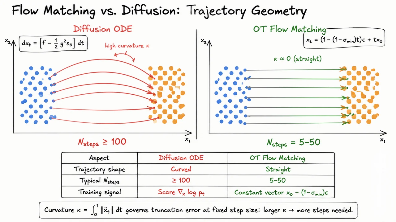
With the geometry of flow matching trajectories now established — straighter interpolation paths that require fewer corrective steps — the natural next question is whether this cleaner geometry pays off where it matters most: on the standardized image-generation benchmarks that the community uses to rank generative models. Geometric elegance is satisfying on its own terms, but FID scores on ImageNet are what move the field. So let us interrogate the empirical record carefully, paying attention to what the comparisons actually control for and where confounders lurk.
The Fréchet Inception Distance (FID) measures the Wasserstein-2 distance between Inception-v3 feature distributions of generated and real images; lower is better. Alongside FID, we track NFEs — number of function evaluations of the neural network during sampling — because NFE is the dominant cost at inference time. A model that achieves FID 2.1 at 50 NFEs is far more practical than one that achieves FID 2.0 at 1000 NFEs. This NFE-FID tradeoff is precisely where the trajectory-geometry story from the previous section should bite: if the learned velocity field points along a nearly straight path from noise to data, an ODE solver can traverse that path accurately with very few steps.
To make this concrete, recall the conditional flow matching objective and the OT interpolant that defines it:
The target velocity is constant along each conditional trajectory — it does not depend on except through the negligible correction. Training to match this target via
therefore asks the network to learn an almost time-invariant direction field, which is a dramatically simpler regression target than the highly curved, time-dependent score function required by diffusion.
Now let us look at what the benchmarks actually show. On CIFAR-10, the picture is mixed and instructive. DDPM (Ho et al., 2020) achieves FID 3.17, but only with 1000 NFEs. DDIM collapses this to ~4.0 at 50 NFEs by switching to a deterministic probability-flow ODE — already a huge practical win that exploits the same trajectory-straightening intuition. Lipman et al.'s flow matching with an OT path achieves FID 6.35 at 100 NFEs, which is worse than DDIM at a higher cost. This is a crucial reality check: on small datasets, OT-path flow matching does not dominate. The marginal path is not automatically easy to learn when the dataset is small and diverse, and the ODE solver's accuracy at modest NFEs depends on how well has actually converged — which requires enough training data and capacity. Stochastic interpolants (Albergo & Vanden-Eijnden, 2022), which blend deterministic and stochastic paths, recover FID 2.99 at ~100 NFEs, suggesting that the specific interpolant matters more than the mere choice of training objective.
The most controlled and convincing evidence comes from the large-scale ImageNet 256×256 setting, where DiT (Peebles & Xie, 2023) and SiT (Ma et al., 2024) provide an almost ideal ablation. Both use the same transformer backbone — the same number of parameters, the same conditioning strategy, the same compute budget — differing only in whether the model is trained with the diffusion objective on a variance-preserving path or with on an OT straight path. At identical NFEs = 250, DiT achieves FID 2.27 and SiT achieves FID 2.06. The gap of 0.21 FID points is non-trivial at this scale; more practically, SiT reaches the same quality as DiT at roughly 10× fewer NFEs, because the straighter velocity field can be integrated accurately with an aggressive step-size schedule.
Several subtleties deserve emphasis. First, the NFE advantage is not free: it relies on using an adaptive or high-order ODE solver (e.g., DPM-Solver++ or a Dormand-Prince method) that can exploit the lower curvature. A naive Euler solver with 25 steps will still be imprecise, but it degrades more gracefully on straight paths than on curved ones. Second, the comparison is meaningful only because architecture and training compute are matched; swapping to a larger or better-tuned diffusion model would likely close or reverse the gap, so one should read the evidence as "flow matching is at least as good as diffusion at fixed architecture" rather than "flow matching always wins." Third, the FID metric itself is notoriously sensitive to the number of generated samples, the choice of reference statistics, and implementation details — a 0.2-FID difference between papers using different evaluation pipelines is nearly meaningless, whereas the DiT/SiT comparison within the same codebase is unusually clean.
The takeaways can be summarized concisely:
The visual below gathers this entire empirical landscape into a single comparison table, ordered chronologically to show how the field has evolved. The SiT row is highlighted to mark the clearest controlled evidence for the flow-matching advantage, and the amber callout below the table isolates the DiT-vs-SiT comparison so the reader can immediately locate the "same architecture, different objective" ablation that makes the result scientifically credible. Reading the table row by row — noting the NFE column alongside the FID columns — makes the core tradeoff vivid: diffusion models often require hundreds to a thousand steps to reach their best FID, while flow matching achieves comparable or superior quality at a fraction of that cost.
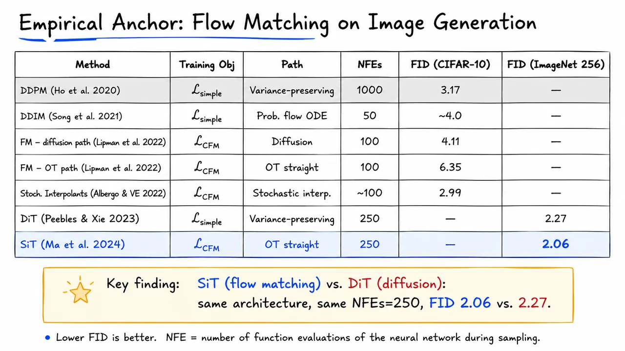
Building on the theoretical machinery we have assembled — the score-matching objective, the ELBO, and the flow-matching regression loss — it is instructive to ground everything in a concrete, low-dimensional setting where we can actually see what each method is doing. The 2D checkerboard is a canonical stress test for generative models: it has eight separated squares on , so a model that collapses even one mode fails visibly, and the geometric structure is simple enough that trajectory shapes are interpretable by eye.
The experimental setup is deliberately controlled. Both DDPM and flow matching are given identical three-layer MLPs with input dimension . The only differences are the training objective and the path interpolation. DDPM uses a cosine noise schedule with discrete steps, predicting the added noise . Flow matching uses the optimal-transport (OT) conditional path with , learning the vector field . Everything else — architecture, optimizer, batch size, number of training iterations — is held fixed. This isolation lets us attribute any performance gap directly to trajectory geometry.
Observation one is about path shape. Under DDPM, the forward process corrupts a data point according to
Because is a nonlinear, monotonically decreasing function of (with cosine shape), the interpolation coefficient is not linear in . As grows, the signal component shrinks quickly at first, then flattens near . This produces curved arcs in data space: the path bends noticeably away from the straight line connecting to . The reverse process must therefore navigate these same curved trajectories in reverse, and a coarse Euler integrator will drift off the true path, accumulating truncation error at every step.
Flow matching with the OT interpolation instead uses
Here, both coefficients are affine in . As a consequence, the conditional path from noise to data is a straight line in , and the corresponding conditional vector field is constant in time:
A constant vector field is the easiest possible target for a neural network — and, critically, it is the easiest possible target for an Euler integrator. When the true velocity does not change along the trajectory, the local truncation error of a single Euler step is exactly zero to first order, regardless of step size. In practice introduces a tiny deviation from perfect linearity, but with this is negligible.
Observation two is about sample quality as a function of the number of function evaluations (NFEs). We measure the Wasserstein-2 distance
between the empirical distribution of 10,000 generated samples and the true checkerboard distribution , sweeping . Flow matching recovers all eight modes cleanly at just , with near its convergence floor. DDPM does not reach the same until , and at ten steps it exhibits visible mode collapse on several checkerboard squares. This is not a failure of the neural network — both networks have converged in training — it is a failure of the ODE integrator when applied to curved trajectories.
The practical implication is significant. If we think of each network forward pass as having a fixed cost, then flow matching achieves equivalent sample quality at five times fewer function evaluations on this benchmark. For high-dimensional image models the cost difference is even starker, because the integration error along curved DDPM paths grows with dimensionality while the OT straight-path argument is dimension-agnostic.
It is also worth asking whether DDPM could use straight paths. In principle, one could choose a linear noise schedule, but the resulting marginals would differ at every intermediate time, and the score function would still be defined by the curved marginal distributions. The key insight of flow matching is that it reframes the training target: instead of learning marginal score functions (an implicit, distribution-level object), we learn conditional vector fields (a per-sample, trajectory-level object), and the optimal choice of those trajectories happens to be straight lines under the OT coupling.
A few sharp takeaways from this comparison:
The visual below consolidates both observations into a single layout. The top row shows the contrast in trajectory shape directly in : curved blue arcs for DDPM versus straight orange lines for flow matching, both plotted against the faint checkerboard background. A side-by-side scatter of generated samples at makes the mode-collapse failure of DDPM immediately visible. The bottom panel presents the versus NFE curves on a log scale, where the steep initial drop of the orange (flow matching) line versus the slow descent of the blue (DDPM) line gives quantitative teeth to everything argued above. Together these panels close the loop from mathematical intuition — straight paths, constant velocity, zero truncation error — to empirical reality on a distribution that is simple enough to be perfectly understood.
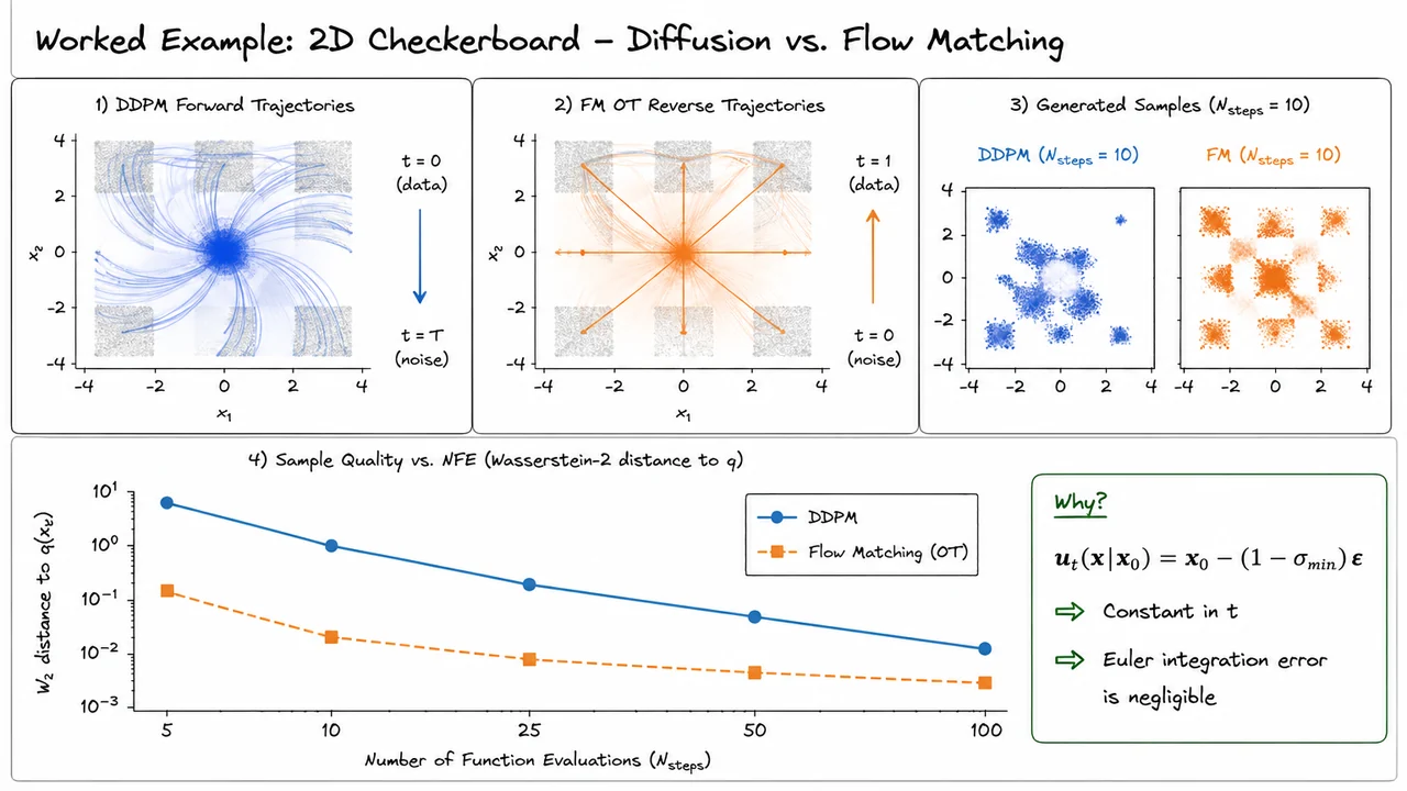
Having worked through the geometry of diffusion versus flow matching on a concrete 2D example, it is natural to ask: can either framework be steered toward a specific output? Random generation is impressive, but essentially every production system in the world—Stable Diffusion, Midjourney, DALL·E—is conditioned on text. The mechanism that makes this work in practice, and the one that controls the classic quality-vs-diversity dial, is classifier-free guidance (CFG).
The core idea is elegant. Instead of training a separate classifier and backpropagating through it at sampling time (the original "classifier guidance" approach), CFG folds conditioning directly into the generative network itself. During training, a single network receives a conditioning signal —a text embedding, a class label, anything—but with probability that signal is replaced by a null token . The network therefore learns two behaviors simultaneously: a conditional denoiser and an unconditional denoiser, sharing all their weights. At sampling time, you call the same network twice per step—once with the real condition, once with —and interpolate extrapolatively:
Reading this algebraically, you are taking the unconditional prediction and moving away from it in the direction of the conditional prediction, with step size controlled by the guidance weight . When you recover the unconditional sample; as grows you amplify the signal that distinguishes the conditioned distribution from the unconditioned one.
Why does this improve fidelity at the cost of diversity? Think of the conditional score decomposed via Bayes: it equals the unconditional score plus . Classifier-free guidance implicitly amplifies that classifier-gradient term by a factor of . A large pushes samples into high-likelihood modes of the conditional distribution—sharp, recognisable outputs—but collapses the diversity because low-probability but valid samples are suppressed. The FID/recall trade-off is not a bug; it is the fundamental geometry of score amplification.
The critical insight for this lecture is that the same formula transfers word-for-word to flow matching. Wherever a DDPM predicted , a flow matching network predicts a velocity field , and the guided velocity is:
The mathematics is structurally identical because both frameworks are learning a vector field over ; guidance is just linear extrapolation in that vector-field space. The training recipe—null-conditioning dropout at rate —is also identical. This framework-agnosticism is one of the reasons CFG became the universal interface for user-controllable generation.
The second major extension is latent diffusion. Running a diffusion or flow-matching process directly in pixel space for high-resolution images is computationally ruinous: a image has nearly 800,000 dimensions. The Stable Diffusion insight (Rombach et al., 2022) was to first train a VAE that compresses images to a latent representation, reducing dimensionality by a factor of 48. The entire generative process—forward noising, score matching, reverse sampling—then operates in this compressed space and the decoder maps back to pixels at the very end. The perceptual quality of the VAE latent space is nearly lossless for natural images, so the generative model inherits image quality while paying only the cost of the latent space. The result is roughly 48× faster sampling with no meaningful degradation. FLUX (Black Forest Labs, 2024) applies the same latent-compression trick but swaps DDPM for flow matching, achieving state-of-the-art text-to-image quality with only neural-function evaluations—a number that would have seemed impossibly low for DDPM-era systems. The straightness of flow-matching trajectories (discussed in the previous sections) is precisely what enables such aggressive step-count reduction.
A few important caveats are worth keeping in mind. First, guidance introduces a hyperparameter that must be tuned per application; too high a value causes oversaturation and artifact-laden outputs because you are extrapolating beyond the support of the learned distribution. Second, the double forward-pass cost at sampling means that in strict latency-constrained settings, people sometimes train networks with guidance baked in (so-called distilled models). Third, the VAE is a fixed, separately trained module, so its reconstruction artifacts set a hard floor on sample quality—no amount of diffusion training can recover detail that the encoder discards.
The visual below consolidates these two threads—classifier-free guidance and latent compression—into one compact reference. The top half places the two guided-prediction formulas side by side under a shared banner noting the null-conditioning training trick, making the structural symmetry between DDPM and flow matching immediately apparent. The bottom half is a comparison table for the two landmark production systems: Stable Diffusion (DDPM, 50 NFEs, latent space, 2022 SOTA) and FLUX (flow matching, 20 NFEs, latent space, 2024 SOTA). Together they illustrate the progression: guidance gives you control, latent compression gives you speed, and the choice of DDPM versus flow matching governs trajectory efficiency—all three levers are independent and composable.
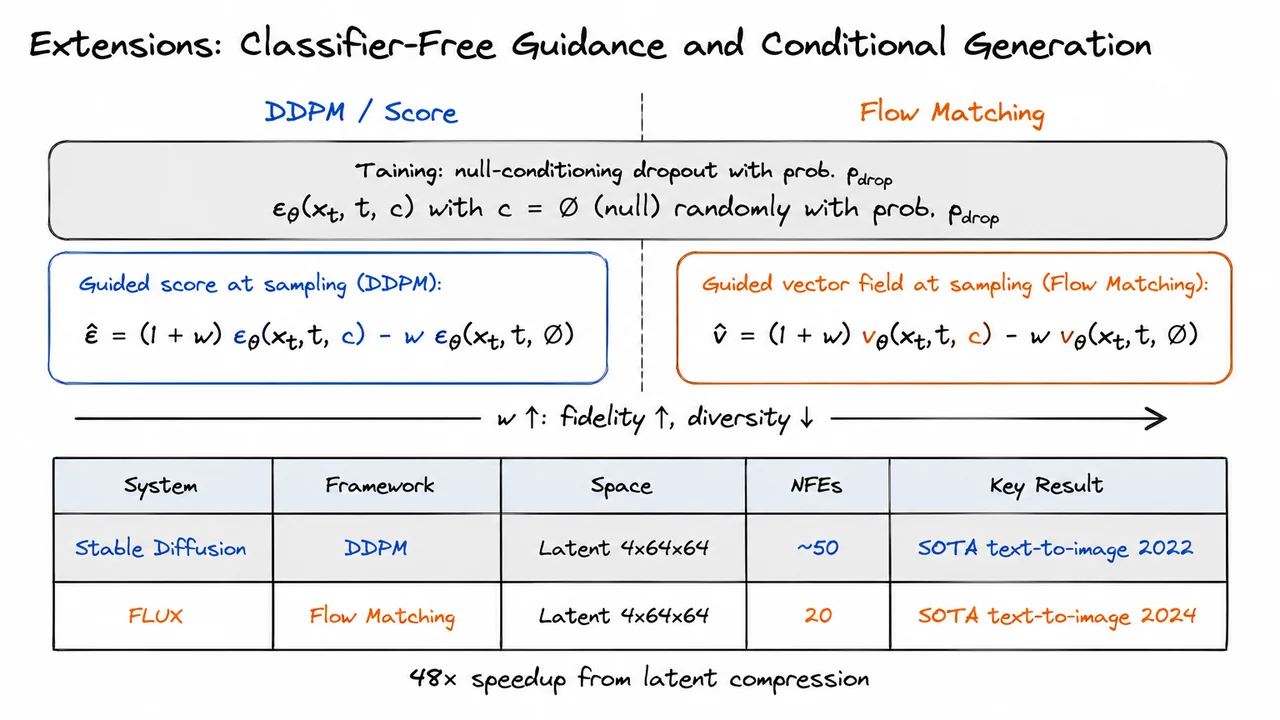
Having traced the full arc from denoising diffusion probabilistic models through score-based SDEs, probability flow ODEs, DDIM, and finally flow matching and stochastic interpolants, it is natural to ask: what actually separates these methods from one another? The answer, once you stand back far enough, is surprisingly compact. The training machinery is almost identical across every variant; what diverges is the geometry of the path each method traces between noise and data.
To make this concrete, recall the two central training objectives we have encountered. For DDPM and its descendants, the simplified loss is
a plain mean-squared error between the injected noise and the network's prediction of it. For flow matching, the analogous conditional flow matching loss is
a mean-squared error between the network's predicted velocity field and the known conditional velocity that moves a sample along a prescribed path. In both cases, computing one gradient step requires exactly one forward pass of the neural network: no ODE simulation at training time, no nested optimization, no second-order information. The per-step training cost is the same across every row of the table we are about to survey.
This equivalence in training cost is not a coincidence—it follows from a deeper structural fact. Every method in this family learns a function that can be evaluated at a single pair to produce a local direction: either the noise residual, the score, or the velocity. The variance-reduction tricks that motivate over the full ELBO, or that motivate conditional flow matching over the marginal velocity formulation, are each just ways to reduce the variance of that single-sample estimate without changing its computational graph. What does change is how much work the trained network must do at sampling time to integrate a trajectory from pure noise to a realistic sample.
This is where path geometry enters as the decisive axis. The DDPM ancestral sampler must take discrete Markov steps because the reverse process is defined as a long chain of small Gaussian transitions; skipping steps breaks the validity of the Gaussian approximation at each one. Score-based SDEs and their probability flow ODE counterparts inherit the same curved paths, and although high-order ODE solvers reduce the required number of function evaluations (NFEs) to the 100–500 range, the underlying curvature of the trajectory demands many evaluation points to maintain integration accuracy. DDIM was the first to observe that you can compress this curved path by conditioning the trajectory on a predicted at each step, bringing NFEs down to 10–100—but the trajectory is still fundamentally curved, just re-parameterized.
Flow matching with optimal-transport couplings (FM-OT) changes the problem at its root. By choosing straight-line interpolants between pairs drawn from an OT plan, the conditional velocity is constant in time. The network therefore needs to learn a velocity field that varies little along each trajectory, and the resulting marginal vector field is nearly straight. Integrating a nearly-straight ODE requires far fewer steps: 5–50 NFEs achieve quality that diffusion samplers need 1000 steps to match. Stochastic interpolants (Albergo 2022) reach the same regime through a slightly different construction—interpolating between source and target with flexible interpolation schedules—but the geometric intuition is identical: straighter paths mean cheaper numerical integration.
It is worth being precise about what "curved" means here. Curvature in the flow sense is not a property of a single trajectory but of the marginal vector field obtained after averaging over all conditional flows. Even if each individual path from to is a straight line, the marginal field can be curved if the conditioning distribution is broad. The OT coupling minimizes exactly the quantity that controls this marginal curvature—the expected squared displacement—which is why it specifically yields straighter marginal flows compared to an independent coupling, and compared to the diffusion process whose reverse flow is defined by the score of a Gaussian-corrupted data distribution.
A subtle but important caveat: straighter paths are not free. The optimal-transport coupling requires pairing samples from data and noise, which at infinite scale is computationally intractable without approximations (e.g., mini-batch OT). In practice, mini-batch approximations introduce a small bias, and the learned velocity field must still generalize across the full data manifold. The empirical evidence—across image, audio, and molecular generation benchmarks—nonetheless consistently shows that FM-OT and stochastic interpolants achieve competitive or superior sample quality at a fraction of the NFEs needed by DDPM or Score SDE.
The key progression, then, is not one of increasing training complexity but of increasing geometric efficiency. Every method in the table pays roughly the same price per gradient step during training. The gain in moving from DDPM to FM-OT is paid back entirely at sampling time, through the ability to integrate a vector field whose paths are close to geodesics in the ambient space.
The visual below crystallizes this comparative analysis into a single reference table, organizing all six methods by training objective, network parameterization, sampler type, NFE budget, and path geometry. The color coding makes the decisive axis immediately legible: the NFE column glows red for the methods that demand thousands of function evaluations, and green for the flow-matching methods that achieve the same task in tens. The two green-bordered rows at the bottom—FM-OT and Stochastic Interpolants—sit in sharp contrast to the four rows above them, not because their training columns look any different, but because their path geometry column reads straight instead of curved. Below the table, the single-line caption captures the entire lesson: training cost per step is roughly one forward pass of the network in every row; sampling cost is the differentiating factor. Everything the lecture has built toward, from the ELBO derivation to score matching to conditional flow matching, converges into that one contrast.
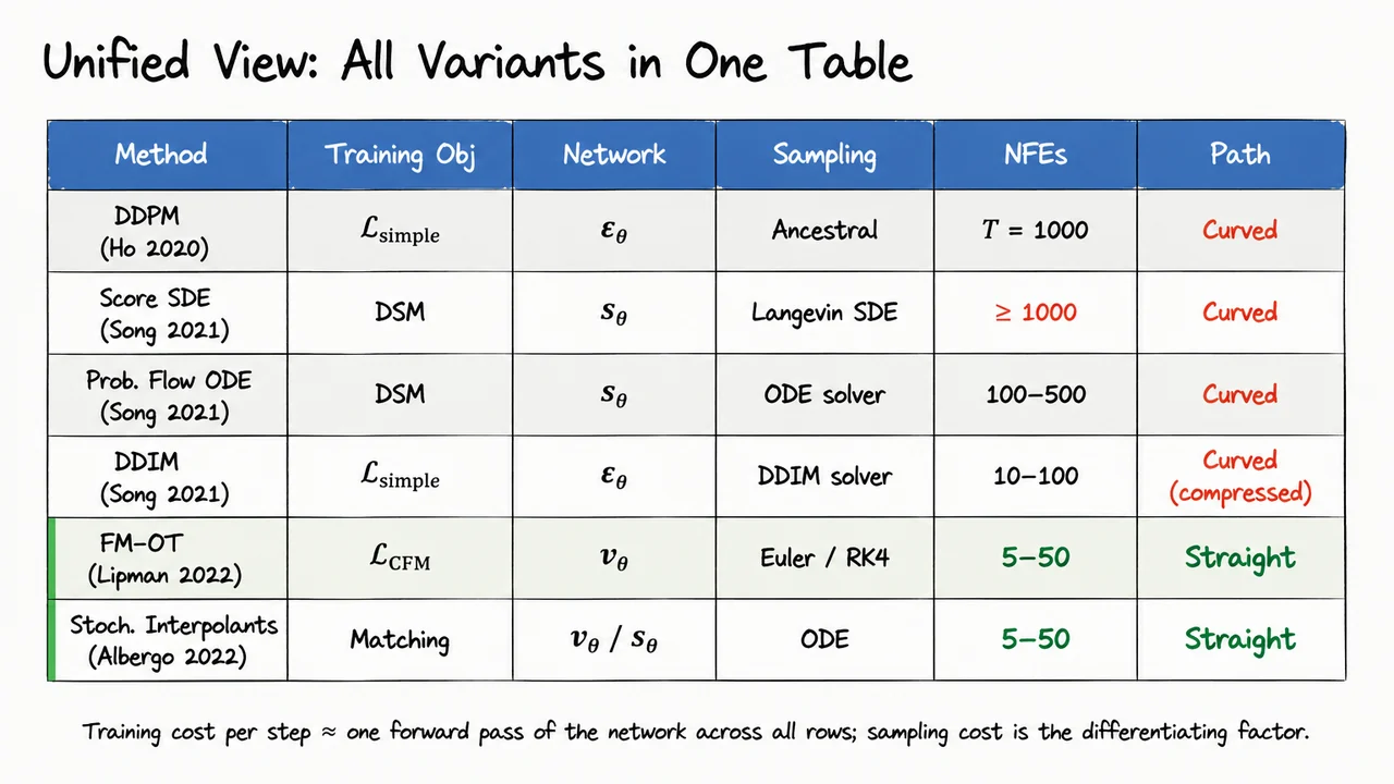
Having now assembled a unified table that places score-based diffusion, DDPM, flow matching, and their stochastic variants side by side, it becomes possible to do something more interesting than merely catalogue them — we can read off the open problems directly from the table's seams. Each row corresponds to a design decision that could, in principle, be made differently, and in most cases researchers are actively exploring exactly that alternative. What follows is a tour of the frontier, organized by the five most structurally important open directions.
Path optimality is perhaps the most immediately actionable gap. Optimal-transport flow matching (OT-FM) earns its name by minimizing expected path length: the coupling is chosen so that the resulting conditional vector field is constant in time, and the marginal flow travels in straight lines. This is geometrically appealing and reduces the number of function evaluations (NFE) needed to integrate the ODE accurately. But "straight" is not the same as "low-perceptual-error at NFE = 1." The open question is whether one can jointly learn the interpolant and the network to minimize a downstream generation metric — say FID — at a fixed and tiny NFE budget. This reframes flow matching as a bilevel optimization problem whose outer objective is non-differentiable with respect to the path family, a genuinely hard problem that current work only partially addresses.
Discrete and structured domains expose the most fundamental assumption buried in every equation we have written so far: that data lives in a continuous Euclidean space where Gaussian noise is a natural perturbation. For text tokens, molecular graphs, or protein sequences, is simply inapplicable. Masked diffusion (Austin et al., 2021) replaces the Gaussian corruption kernel with a categorical one — typically an absorbing mask state — and the score function is replaced by a ratio of categorical probabilities. The flow-matching perspective for discrete spaces is even less settled; recent work (Campbell et al., 2022) develops continuous-time Markov chain analogues, but the theory is far less mature than its continuous counterpart.
Consistency models (Song et al., 2023) attack the NFE problem from a completely different angle: rather than designing straighter trajectories, they enforce a self-consistency constraint directly on the learned function. Recall the probability flow ODE from earlier in this lecture:
Every point along a deterministic trajectory of this ODE maps to the same clean image . Consistency models parameterize a function and train it to satisfy
so that a single network evaluation from any noise level produces the same clean prediction. This is conceptually identical to one-step flow matching, but it achieves its objective by distillation rather than by designing the path family. The consistency distillation variant bootstraps from a pre-trained diffusion model, while consistency training attempts to learn the property from scratch — each with its own stability and bias tradeoffs.
Optimal control and the Schrödinger bridge reveal that the reverse SDE is not merely an empirical trick but has deep roots in variational mechanics. Berner et al. (2022) showed that training a reverse diffusion is equivalent to solving a stochastic optimal control problem:
The objective penalizes the kinetic energy of the control , and the constraint says the controlled process must end at the data distribution. When we additionally require the process to start from a fixed prior, this becomes the Schrödinger bridge problem — the entropy-regularized optimal transport between and . OT flow matching, as we have seen, recovers the static (zero-entropy-regularization) limit of this bridge. The full dynamic Schrödinger bridge, solved iteratively via IPF (De Bortoli et al., 2021), generalizes both and opens connections to thermodynamics and stochastic control theory that are still being actively mined.
Scaling laws bring the discussion back to empirical engineering. Chen et al. (2024) demonstrated that flow matching models on ImageNet exhibit power-law scaling: , mirroring the now-famous scaling laws for large language models. This is significant because it suggests that the architectural and data scaling intuitions developed for transformers may transfer directly to continuous generative models — and conversely, that hardware and dataset investments will yield predictable returns. It also raises the question of whether score-based diffusion and flow matching have different exponents, which would favor one paradigm at scale.
These five directions are not independent. Consistency models can be viewed as a special case of the optimal-control formulation with a terminal cost; discrete diffusion requires rethinking both the path family and the self-consistency constraint; and scaling laws apply differently depending on how many steps are used at inference. What makes this moment in the research landscape unusual is that theoretical and empirical frontiers are advancing simultaneously — a rare alignment.
The visual that follows organizes these five open problems into a compact two-column reference map. On the left, each problem is annotated with its defining equation or key constraint; on the right, the corresponding literature is pinned as a reading list. Arrows connecting each block to its citations make explicit which theoretical claim is grounded by which paper. Reading the diagram from top to bottom traces a path from geometry (path optimality) through structure (discrete domains) through engineering (consistency distillation) through theory (optimal control) to empirics (scaling laws) — a natural arc that reflects how the field itself is maturing. The diagram does not replace the equations or the arguments above, but it gives the reader a single reference card to hold the entire frontier in working memory.
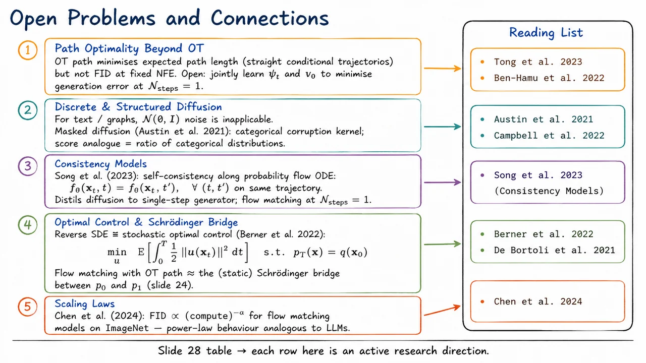
Generative modeling sits at the heart of modern machine learning, yet the problem it poses is deceptively simple to state and brutally hard to solve. We are handed a finite collection of observations — photographs, audio clips, protein structures, text documents — and asked to learn the hidden probability distribution that produced them well enough to both evaluate and sample from it. Everything else in this lecture grows out of understanding precisely why that is difficult.
Formally, suppose we observe a dataset , where each . For a standard RGB image at 256×256 resolution, . Our task is to find parameters such that a model distribution satisfies
A useful generative model must satisfy two simultaneous desiderata. First, it should assign high likelihood to real data — meaning should be large wherever is large. Second, it should support efficient, diverse sampling — drawing fresh examples that look indistinguishable from real ones in finite compute time. These two goals are more in tension than they might first appear; many architectures that excel at density estimation are slow to sample from, and vice versa.
The root cause of almost every difficulty is the curse of dimensionality. The most naïve approach to density estimation is a histogram: discretize each dimension into bins, count how many samples fall into each cell, and normalize. The number of cells scales as , so even with bins per dimension and , the histogram has more cells than there are atoms in the observable universe. Kernel density estimation (KDE) fares no better asymptotically — its sample complexity grows exponentially in . The ambient space is simply too large to cover with any finite dataset.
What saves us — partially — is the manifold hypothesis: real data does not spread uniformly over . Natural images, for instance, live on a vastly lower-dimensional manifold embedded in pixel space. Randomly-sampled Gaussian vectors in look like snow; real images occupy an astronomically small corner of that space. This means the effective complexity of the problem is much lower than the ambient dimension suggests — but we have to build a model that discovers and exploits that low-dimensional structure without ever being told what it is.
Parametric models — neural networks, normalizing flows — try to encode this structure implicitly. But a second fundamental obstacle arises immediately: computing the normalizing constant
is generally intractable for flexible models. If we parameterize an energy-based model , for instance, the integral over all of is unavailable in closed form, blocking both maximum-likelihood training and exact sampling. Normalizing flows avoid this by restricting to invertible architectures with tractable Jacobians — an elegant fix, but one that constrains expressivity and is computationally expensive at scale.
The conceptual breakthrough that motivates this entire lecture is a different kind of resolution: rather than trying to model directly, decompose the problem through a noise schedule. We design a process that gradually corrupts a data point into pure Gaussian noise over steps. This forward process is easy and known by construction. The hard distribution is then recovered by learning to reverse this corruption — denoising noise back into data, one small step at a time. Each individual denoising step operates on a nearly-Gaussian local distribution, sidestepping the global normalization problem entirely.
This noise-based decomposition is elegant for several reasons. It replaces one intractable global problem with a sequence of tractable local problems. It naturally exploits the manifold structure of data, because the noising process smoothly interpolates between the sharp data manifold and a featureless Gaussian. And it connects to deep mathematical tools — stochastic differential equations, score functions, and optimal transport — that we will develop carefully throughout this lecture.
The visual below captures both the difficulty and the proposed resolution in a compact diagram. On one side, it depicts the core tension: data lives on a tiny, irregular support within the vast ambient space , while the model must simultaneously achieve high likelihood and efficient sampling from that distribution. On the other side, the noise-decomposition idea appears as a bridge — a continuum connecting structureless Gaussian noise to the rich, structured data distribution. This bridge is exactly the object we will learn to traverse, and building it rigorously is the subject of everything that follows.
Having established that the core challenge in deep generative modeling is faithfully learning an intractable data distribution from finite samples, it is tempting to ask: haven't we already solved this? Three families of models dominated the field for years — Variational Autoencoders, Generative Adversarial Networks, and Normalizing Flows — and each represents a genuinely clever engineering compromise. The trouble is that each compromise carries a structural flaw that cannot be patched away with more computation or better architecture. Understanding why these flaws are fundamental is exactly the motivation for everything that follows.
Variational Autoencoders take the most principled probabilistic route. The core idea is to introduce a latent variable and optimize a tractable lower bound on the log-likelihood:
The first term rewards accurate reconstruction; the second term regularizes the approximate posterior toward a prior. The critical subtlety is that is a parameterized approximation to the true posterior . Because these two distributions are never exactly equal — a gap that persists at convergence whenever the true posterior is multimodal or has complex geometry — the decoder must effectively average over a smeared-out region of latent space rather than a single precise encoding. This averaging is precisely what produces the notorious blurriness of VAE samples: the reconstruction loss, typically mean-squared error, has the statistical effect of regressing toward the mean of the posterior distribution, washing out sharp high-frequency detail.
Generative Adversarial Networks abandon likelihood altogether in favor of an adversarial game. A generator and discriminator are trained under the minimax objective:
In theory, the unique Nash equilibrium of this game recovers the true data distribution. In practice, the generator can satisfy the discriminator perfectly by placing all of its probability mass on a single sharp mode of . Because the discriminator sees realistic-looking samples and cannot easily penalize the generator for failing to cover the other modes it has never observed, training dynamics fall into mode collapse — a pathology that is both difficult to detect during training and notoriously hard to cure. The fundamental problem is that the generator's objective provides no explicit incentive to maintain coverage of the full data distribution.
Normalizing Flows return to exact maximum likelihood by constructing a sequence of invertible transformations that map a simple base distribution into the data distribution. By the change-of-variables formula:
This is mathematically exact — no approximation, no adversarial game. The problem is computational. For a -dimensional random variable, the Jacobian is a matrix, and computing its determinant naively costs . For images with or , this is completely infeasible. Practitioners must therefore restrict their networks to volume-preserving coupling layers (as in RealNVP or Glow), whose structured form makes the Jacobian triangular and the determinant cheap to compute — but at the cost of severely limiting the expressive power of the transformation. You can have exact likelihoods or expressive architectures, but not both.
The pattern is worth pausing on:
Each method essentially purchases tractability by giving something up. No combination of tricks within any single framework resolves all three problems simultaneously, because each failure mode is a direct consequence of the framework's defining design choice.
Diffusion models sidestep this trilemma through a conceptually different move: instead of designing a clever approximate inference scheme, an adversarial game, or a constrained invertible network, they commit to a fixed, analytically tractable forward process that progressively destroys structure in the data. Because the forward process is given — not learned — there is no posterior gap to approximate, no discriminator to fool, and no Jacobian to compute. The model need only learn to reverse a process whose statistics are fully known. This might sound like it merely pushes the problem elsewhere, but as the next section will show, the reverse process turns out to have exactly the right mathematical structure to be learned efficiently with a simple regression objective.
The visual below consolidates this three-way comparison in a compact side-by-side layout. Each column captures one method's schematic and its critical failure mode — the posterior mismatch in the VAE column, the collapsed generator samples in the GAN column, and the cost annotation on the flow column. The bottom strip unifies all three under a single verdict: in every case, something fundamental is sacrificed. Seeing the three failures lined up in parallel makes it easier to appreciate that diffusion models are not just an incremental improvement on any one approach — they represent a qualitatively different answer to the same underlying question.
Having established why prior generative approaches struggle — GANs require delicate adversarial balance, VAEs are constrained by their encoder bottleneck, and normalizing flows demand architecturally expensive invertibility — we can now ask a sharper question: is there a way to turn density estimation into something more like ordinary supervised learning? Diffusion models answer that question with a surprisingly elegant reframing.
The key philosophical shift is to stop trying to learn the data distribution all at once. Instead, observe that destroying structure is trivially easy: add a small amount of Gaussian noise to a clean image, and you get a slightly noisier image. Repeat this operation hundreds of times, and the original signal is completely overwhelmed. After enough steps, the distribution of the corrupted sample is indistinguishable from an isotropic Gaussian, regardless of what looked like to begin with. Formally, the forward process defines a Markov chain:
This direction requires no learning whatsoever. It is a fixed, hand-designed process that we only run at training time. Its sole purpose is to create a bridge between the rich, complicated data distribution and a simple, well-understood prior.
The generative power of diffusion models comes entirely from learning to invert this process. The reverse process attempts to walk the same chain backwards:
Sampling then becomes: draw pure noise , and iteratively apply the learned reverse steps. Each step removes a small, controlled amount of noise, slowly sculpting structure out of chaos until a plausible data sample emerges.
Why is the reverse direction tractable when the forward direction is trivially easy and single-step density estimation is famously hard? The critical insight is one of locality. At each reverse step , the noisy sample is already very close to the distribution it came from, . The reverse conditional is approximately Gaussian when the forward step adds only a small amount of noise. This means the network does not need to solve the full inverse problem in one shot — it only needs to answer the narrow local question: given that I am at , which direction reduces noise by one small step?
Concretely, a neural network is trained to predict the noise vector that was added to a clean sample to produce . The training loss is simply mean squared error:
The elegance here is hard to overstate. There is no adversarial game — no discriminator, no Nash equilibrium to worry about. There is no constraint on the network's Jacobian. There is no encoder–decoder bottleneck. The training signal is just a regression target: the noise that was sampled and applied, which is known exactly at training time. Any architecture capable of regressing vector fields — typically a U-Net or a Vision Transformer conditioned on the timestep — can serve as .
It is also worth pausing on why predicting noise is equivalent to something deeper. The score function of a distribution is , the gradient of the log-density with respect to the input. It turns out that the noise-prediction network is directly proportional to the score of the noisy distribution: knowing the noise added is the same as knowing how to increase the log-probability of the data. This connection — which we will derive formally in later sections — gives diffusion models a solid probabilistic foundation and explains why the simple MSE objective is not just a heuristic but is grounded in maximum likelihood reasoning.
The practical consequences are significant. Because each reverse step is a small, local regression, the network can be trained stably on massive datasets. The same checkpoint can generate samples of arbitrary resolution (within the trained distribution) by simply running the chain. And because the forward process is fixed, there is no mode collapse — the network cannot "ignore" parts of the data distribution the way a GAN generator can.
The visual below crystallizes this two-track structure. The top lane shows the forward process: a clean image dissolving into Gaussian static as controlled noise accumulates step by step. The bottom lane shows the reverse process running in the opposite direction, with the learned network guiding each denoising step. The pure-noise boundary at acts as the shared anchor: the forward process ends there deterministically, and the reverse process begins there stochastically. At the base of the diagram, the MSE training objective anchors the whole picture, reminding us that the formidable-sounding problem of learning a generative model over high-dimensional images reduces, at every gradient step, to predicting a Gaussian noise vector — a regression problem any modern neural network can solve.
With the intuitive picture of progressive noising and denoising now in hand, it is time to make everything precise. Good notation is not bureaucracy — in diffusion models, the specific parameterization choices baked into the forward kernel are what make the entire training procedure tractable, and a single carelessly defined symbol can obscure a beautiful closed-form result that would otherwise save enormous computation. So let us build the scaffolding carefully.
The forward process is defined as a discrete-time Markov chain of length , operating on random variables . The data sample is drawn from the unknown data distribution . Each subsequent variable is produced by a single Gaussian step:
Every step does two things simultaneously: it shrinks the mean by a factor of and injects fresh Gaussian noise with variance . The shrinkage is essential — without it, the variance would grow without bound. With it, one can show that as the marginal converges to a standard normal, regardless of what looked like. The noise schedule is a design choice: early steps add little noise (preserving fine structure), while later steps destroy information aggressively. Typical schedules are linear, cosine, or learned.
To keep notation compact, define:
Think of as the signal retention factor at step : it is close to 1 when is small (early, low-noise steps) and falls toward 0 as noise accumulates. The cumulative product is the key quantity in the entire framework. It measures how much of the original signal survives after noising steps. When , the sample is nearly clean; when , the sample is nearly pure noise. We will see in the next section that lets us jump directly from to any without simulating every intermediate step — a property that is absolutely critical for efficient training.
Because the forward process is Markov, the joint forward distribution over the entire trajectory factors as a product of one-step kernels:
There are no parameters to learn here; is entirely fixed by the schedule . This is a crucial asymmetry: the forward process is a known, deterministic recipe, while the reverse process must be approximated.
The reverse generative process mirrors the Markov factorization but runs backwards and uses learned parameters :
Generation begins by sampling from a standard normal — cheap and parameter-free — and then iteratively applies learned denoising kernels to recover a sample that looks like it came from . In practice each is itself taken to be Gaussian, with a mean predicted by a neural network and a fixed or learned variance. The Gaussian assumption in the reverse process is not trivially justified — it holds approximately when each is small, because the true reverse posteriors are then nearly Gaussian. This is why small step sizes (large ) matter.
Finally, it is worth naming the signal-to-noise ratio now, even though it plays a starring role only in later derivations:
The SNR decreases monotonically from (where it is high, close to ) down to nearly zero at . This quantity reappears naturally when bounding the ELBO, when choosing loss weightings, and when comparing different noise schedules. The conceptual message is simple: tracks signal, tracks noise power, and their ratio summarizes the information content at each timestep.
The visual below consolidates the entire notational setup into a single reference diagram. On one side, the core equations are laid out in their logical order — the forward kernel, the definitions, the joint factorization, the reverse factorization, and the SNR — numbered so you can cross-reference them as derivations proceed. On the other side, a vertical timeline makes the Markov structure legible at a glance: (a structured data point) sits at the top, sits at the bottom, and the forward arrows () and dashed reverse arrows () run in opposite directions along the same chain. Below the chain, a simple bar chart illustrates the noise schedule: climbs monotonically while falls, converging to zero as the SNR bottoms out.
Together, the equations and the diagram make concrete what might otherwise feel like a tangle of subscripts: there are exactly two processes, one fixed and one learned, they share the same Markov graph, and the single number is the bridge that will let us derive everything that follows without ever simulating the chain step by step.
Having established the Markov chain structure of the forward process — where each step applies a small Gaussian perturbation to the previous sample — a natural and practically critical question arises: do we really need to simulate all steps of the chain every time we want to train the model? At first glance, computing from seems to require iterating through sequential transitions, which would make training prohibitively expensive for large . The key insight of DDPMs is that the Gaussian structure of the forward kernel makes this chain collapsible — we can jump directly from to any in a single step.
To see why, start from the one-step reparameterization implied by the Markov kernel , where we define . Writing this in reparameterized form:
Now unfold one additional step by substituting with an independent noise draw :
The two noise terms are independent Gaussians, so their sum is itself Gaussian with variance . The elegant algebraic fact is that this simplifies to , because . Folding the two noise terms into a single gives:
This is structurally identical to the one-step formula, with playing the role of the single-step . The pattern is unmistakable, and induction closes the argument immediately. Applying the same merging procedure times and defining the cumulative noise schedule , we arrive at the closed-form marginal:
or equivalently in the reparameterized sampling form:
It is worth pausing to appreciate the geometry encoded in this result. The noisy sample is a linear interpolation in variance space between the clean signal and pure isotropic noise: the coefficient scales the signal component, while scales the noise component, and the two squared coefficients sum exactly to one. As , and the distribution of collapses to — the data is fully destroyed. Near , and is nearly unchanged. The schedule (and hence ) controls how quickly this transition happens, with linear, cosine, and learned schedules each offering different tradeoffs in practice.
The practical consequence is profound. During training, we need to evaluate the model's denoising ability at a randomly chosen timestep for each mini-batch example. Without this closed form, that would require simulating the entire Markov chain from to , meaning sequential Gaussian samples. With the closed form, we instead draw , sample , compute , and immediately present the corrupted image to the network. The entire forward pass is regardless of , which is what makes DDPM training scalable to thousands of timesteps.
One subtle assumption underlying this derivation is the independence of noise draws at each step of the chain. Because we condition on the current state when sampling the next, the individual terms are independent by the Markov property — and it is exactly this independence that allows us to merge them into a single equivalent Gaussian. If the noise were correlated across steps (as in some non-Markovian variants explored later), the composition would not simplify so cleanly. This independence is not just a convenience; it is a structural prerequisite for the entire derivation.
The visual below distills this derivation into three logical layers that mirror the argument exactly. The top panel captures the two-step composition, showing how two sequential reparameterizations merge into one via the variance identity . The central panel presents the boxed main result — the closed-form marginal — highlighted to signal that this is the destination of the inductive argument. A small downward arrow labeled "apply times" bridges the two-step example to the general formula, making the inductive logic visually explicit.
The bottom panel reinforces the payoff: the reparameterized sampling equation and the consequence. A compact timeline diagram on the right margin shows the contrast most vividly — intermediate nodes are grayed out and bypassed, with a bold direct arrow leaping from to labeled by . That single arrow captures the entire point: a quantity that was seemingly chained across steps collapses, through the magic of Gaussian closure, into one line of arithmetic.
Having established that the forward process collapses any data point into near-isotropic Gaussian noise in closed form, the natural next question is: how do we train the reverse process at all? The marginal log-likelihood requires integrating over every possible noisy trajectory , which is combinatorially intractable. The classical remedy — borrowed straight from variational inference — is to construct a lower bound on that log-likelihood and maximize the bound instead.
The variational lower bound (ELBO) arises by a single application of Jensen's inequality. Because is concave, we can multiply and divide the joint model density by the forward-process distribution and push the expectation outside the log:
This is identical in spirit to the VAE objective, with one crucial difference: the "encoder" here is the fixed forward diffusion process rather than a learned amortized network. That fixedness is both a gift and a constraint — it means we never have to worry about posterior collapse or encoder training instability, but it also means the variational gap is baked in by the noise schedule rather than being adaptively minimized.
The bound as written is still a monolithic expectation over all latents simultaneously. To make it actionable, we exploit the Markov structure of both the forward and reverse chains. Writing out the joint densities in terms of their conditional factors and canceling telescoping terms, the ELBO neatly separates into three semantically distinct pieces:
Each term has a distinct role, and understanding that role is the key to understanding why DDPMs are trainable at all.
The reconstruction term measures how well the learned reverse kernel recovers the original data from a lightly noised version. This is the only term that directly involves the data likelihood, and it is fully tractable to evaluate by sampling and evaluating the model's log-probability.
The prior-matching term penalizes any mismatch between the final noisy distribution and the standard Gaussian prior . Here is where the noise schedule design from the previous section pays off: by construction, , so regardless of . Consequently is essentially constant in and can be safely ignored during optimization. This is not an approximation we make for convenience — it is a design guarantee.
The denoising matching terms are where all the interesting training happens. Each one is a KL divergence between the reverse model kernel and the forward-process posterior . The latter, conditioning on both the current noisy state and the clean image, is a tractable Gaussian — a fact we will derive carefully in the next section. This tractability is the linchpin of the entire training algorithm: instead of asking "what is the reverse dynamics?", we ask "how closely does the model posterior match the Bayesian posterior conditioned on the data?" That question has an analytic, closed-form answer for Gaussian distributions, reducing each to a simple squared-distance between Gaussian parameters. The sum over then decomposes the training objective into independently optimizable terms, each targeting a single denoising step.
A subtle but important point: the conditional posterior is only tractable because we condition on . If we tried to compute without that conditioning, we would need to marginalize over all data points, which loops us back to the original intractability. The ELBO decomposition is clever precisely because it restructures the problem so that every term involves a quantity we can compute given a training sample .
It is also worth noting what this decomposition implies about the training loop. At each gradient step, we:
No simulation of the reverse chain is required during training. This is a critical practical advantage — in contrast to methods that must actually run the generative model forward to estimate gradients.
The visual below organizes this decomposition at a glance: the two key equations appear in shaded boxes, and below them a color-coded table separates the three terms by their gradient status. Green marks the reconstruction term (trainable), gray the prior-matching term (constant, ignored), and red the denoising terms (the main training targets). A callout arrow bridges the algebra in the second equation to the red row, making explicit that it is the sum — not the full ELBO monolith — that the optimizer actually touches. A blue box at the bottom crystallizes the key insight: the entire burden of learning falls on matching to a posterior we can compute exactly, one timestep at a time. Seeing the three rows laid out in isolation makes it immediately clear why the DDPM loss is so well-conditioned: the hard terms are constant, and the tractable terms each involve only a single Gaussian KL.
Having decomposed the ELBO into a sum of KL divergences, we face an immediate practical question: what exactly are we trying to match? Each KL term asks us to push the learned reverse distribution close to the true one-step backward conditional . The remarkable fact — one that makes DDPMs trainable at all — is that this backward conditional, while it would ordinarily be intractable, becomes an explicit Gaussian the moment we condition on the clean image . Let us derive this carefully.
The key move is Bayes' rule applied within the Markov structure of the forward process. Because the forward chain is Markov, we can write
The left-hand factor is the single-step transition, and the right-hand factor is the marginal obtained by running the forward process from for steps. Both of these are Gaussians we already have in closed form from the reparameterization of the forward process. Specifically,
Substituting these and taking the product of the two exponential kernels gives an unnormalized density in that is itself a Gaussian — but you have to complete the square to read off the parameters. Grouping the terms from both quadratics yields a precision (inverse variance) equal to
The posterior variance interpolates between (which would be the variance if we knew absolutely nothing about ) and something smaller, because the marginal provides additional information that sharpens the distribution. Notice that as , , so and the posterior collapses to a point — which makes perfect sense, because one diffusion step away from the clean image there is almost no uncertainty left given .
Reading off the mean of the completed square is equally illuminating. The posterior mean is
This is a convex-like weighted combination of the clean image and the noisy image . The weights are not arbitrary: the coefficient is large when is large (lots of noise was added at this step, so the clean image is very informative for denoising), while the coefficient is large when is large (we are far along the noising trajectory, so the current noisy state itself carries meaningful signal about where we were one step earlier). The two regimes blend smoothly across the whole diffusion timeline.
At this point the derivation is complete — but there is a crucial subtlety for test-time use. During training we have access to , so we can evaluate exactly. At inference, however, is the very thing we are trying to generate. Fortunately, the reparameterization trick from the forward process gives us an algebraic relationship:
where is the noise that was added to reach . At test time we replace with the network's prediction , giving an estimated . Substituting this estimate into the mean formula yields a fully computable reverse step — and, as we will see in the next section, this substitution also reveals why the ELBO collapses to a simple noise-prediction loss.
It is worth pausing to appreciate why this tractability is non-trivial. In a generic latent-variable model, the posterior would require integrating over complex non-linear transformations and would have no closed form. Here the entire chain is linear-Gaussian, which means Bayes' rule on products of Gaussians stays Gaussian. The DDPM design — using additive Gaussian noise with a variance schedule — is not just a convenient choice; it is the specific structure that makes the target distribution analytically tractable and therefore makes the KL in the ELBO computable without a variational approximation for .
The visual below consolidates this three-step derivation into a single structured layout. Starting from the Bayes' rule factorization at the top, the diagram traces the substitution of the forward Gaussians through the completing-the-square step, arriving at the two boxed results — and — as highlighted final quantities. A third block then shows the test-time substitution formula for in terms of the noise network, making explicit how the analytically derived mean connects to the trainable component of the model.
Seeing all three pieces together in this way clarifies the logical dependencies: the posterior variance depends only on the noise schedule and is fixed before training begins; the posterior mean depends on , which during training is observed and at inference is replaced by a neural prediction. That clean separation between fixed geometry and learned content is what gives DDPMs their elegant training objective.
With the tractable posterior firmly in hand, we are finally in a position to ask the most practical question in the whole DDPM framework: what exactly should a neural network be trained to do, and what loss function should we optimize? The derivation that follows is perhaps the most important result in the diffusion model literature — not because it is mathematically deep, but because it is surprisingly simple, and that simplicity turns out to be a design choice, not a derivation necessity.
Recall that the full ELBO for a DDPM decomposes into a sum of KL divergence terms, one for each denoising step . Each term measures how well the learned reverse conditional matches the true posterior . Because both distributions are Gaussian, each KL reduces to a mean-squared difference between their respective means — and after substituting the reparameterization of the forward process, those means can be written entirely in terms of the noise that was added. Specifically, the forward process satisfies the closed-form expression
which means that sampling a noisy image at any timestep is just a single, embarrassingly cheap operation — no sequential simulation needed. This is often called the reparameterization trick for the forward process, and it is what makes the following simplification tractable.
When you work through the algebra, each KL term in the ELBO becomes proportional to
where the network is trained to predict the noise that was mixed into to produce . The ELBO weighting coefficient is
where is the posterior variance and . This is a complicated, timestep-dependent scalar. For small (low noise), is tiny and this weight is near zero, meaning the ELBO barely penalizes errors at easy, nearly-clean timesteps. For large (heavy noise), the weight grows but in a non-uniform way that is dictated purely by the noise schedule arithmetic.
Ho et al. (2020) made the empirically motivated decision to drop entirely and replace it with a constant weight of . The result is the simplified objective:
This is just an MSE loss on noise prediction, averaged uniformly over all timesteps, all data points, and all noise draws. The relationship to the ELBO is clean: is a reweighted version of the ELBO, with the theoretically correct weights replaced by uniform weights. The trade-off is illuminating:
Why should this up-weighting help? Intuitively, getting the coarse, high-noise denoising right has a large effect on the macroscopic structure of the generated image. The ELBO, which is derived as a lower bound on log-likelihood, cares most about the fine-grained steps where the distribution is concentrated near real data — but perceptual sample quality is governed by whether the model correctly captures the rough composition of a scene, which lives at high noise levels. The simplified objective implicitly acknowledges this by allocating equal training pressure across all noise scales.
There is a subtle but important subtlety worth pausing on: is not guaranteed to improve the marginal likelihood. It is a heuristic deviation from the ELBO, and in principle one could find settings where the weighted ELBO trains a model with higher likelihood. The empirical finding that the simplified loss produces better-looking samples tells us that DDPM training is not primarily about maximizing likelihood — it is about learning a good noise-to-image mapping across all scales. This philosophical point connects to the broader debate between likelihood-based objectives and perceptual quality in generative modeling.
Algorithmically, the training loop that follows from is remarkably clean: sample from data, sample uniformly, sample , construct in one shot, forward-pass through , and take a gradient step on the squared error. No simulation of the Markov chain is needed during training. This simulation-free property, inherited directly from the closed-form forward process, is one of the core reasons DDPMs are practical to train at scale.
The visual below consolidates exactly this comparison. At the top, the theorem statement anchors the derivation with the closed-form forward process and the MSE loss. The side-by-side comparison beneath it — the complicated fraction on the left versus the constant on the right — makes the design choice tangible: one weighting is what the math demands, and the other is what works in practice. This gap between theoretical optimality and empirical performance is a recurring theme in deep generative modeling, and seeing it laid out side by side makes the theorem feel less like a formal result and more like a principled engineering decision backed by evidence.
Having established the form of the ELBO and identified its dominant terms as KL divergences between consecutive-step distributions, the natural next question is: why does minimizing this complex variational bound reduce, in practice, to something as clean as predicting Gaussian noise with mean-squared error? The answer lies in a beautiful chain of substitutions, each one stripping away a layer of complexity until only the essential signal remains.
The first key observation is a standard fact about Gaussian distributions: the KL divergence between two Gaussians that share the same covariance depends only on their means. Concretely, if both and are , the general KL formula collapses entirely to a squared Euclidean distance between their means, scaled by the shared variance:
The design choice to fix the variance of the reverse process to the same schedule as the tractable posterior is therefore not cosmetic — it is what makes the objective analytically tractable. If the variances differed, the KL would carry additional log-determinant terms that would couple the variance and mean learning problems together.
The second move is to choose a specific parameterization of the learned mean . Rather than having the network directly predict the denoised mean, Ho et al. mirror the functional form of the true posterior mean , but replace the true noise with a neural network prediction :
This is a re-parameterization in the spirit of the reparameterization trick — instead of predicting a point in data space directly, the network predicts the noise that was mixed in during the forward process. The structural advantage is that already tells us the ground truth: the "correct" noise is exactly . Knowing this, we can also re-express the true posterior mean by inverting the forward process equation to write and substituting:
The structural symmetry here is striking: both and have identical scaffolding — the same prefactor , the same term, and the same coefficient — differing only in whether the noise slot is occupied by the true or the predicted . This means the difference of the two means collapses cleanly:
Substituting this into the KL expression, we get a weighted noise-prediction MSE at each timestep:
The full ELBO is a sum of such terms over , each carrying its own time-dependent weight . In principle, one could train with these exact weights, and some follow-up works explore the benefits of doing so. However, Ho et al. found empirically that dropping the weighting entirely — treating every timestep as equally important by setting and sampling uniformly — leads to better sample quality. The resulting objective is the celebrated simplified loss:
Why does dropping the weights work? Intuitively, down-weights timesteps near where the noise level is high and the signal-to-noise ratio is low — but those steps contribute substantially to perceptual quality. Equalizing the weights implicitly up-weights the high-noise regime, encouraging the model to learn coarse structure as well as fine detail, which turns out to be beneficial for image generation.
It is worth pausing on what makes this proof non-trivial. The whole reduction depends on three independently motivated design decisions clicking together: (1) matching the variances of the forward posterior and the reverse model, (2) parameterizing the reverse mean in the noise-prediction form, and (3) expressing the true posterior mean via the forward process reparameterization. Any one of these could have been done differently — and the ELBO would still be a valid bound — but only this combination produces the satisfying cancellation above.
The visual below traces exactly this chain of five algebraic steps, arranged as a vertical proof flow. Each step is annotated with the key substitution being made — from the KL simplification for equal-variance Gaussians, through the noise reparameterization, to the mean-difference collapse — culminating in the final weighted MSE and the simplified form with weights dropped. Seeing the steps in sequence makes viscerally clear how the structural symmetry between and is by construction, not by coincidence, and why the final objective is both correct and surprisingly simple.
Having worked through the ELBO and its simplification, we now arrive at the satisfying payoff: the full training and sampling procedures collapse into two clean, implementable loops. This is the moment where the theoretical machinery earns its keep — everything that looked complicated reduces to something a practitioner can actually run.
Training a DDPM is remarkably cheap per step. The key insight, established when we derived the reparameterized forward process, is that we never need to simulate the Markov chain one step at a time. Given a clean data sample , we can jump directly to any noise level in closed form:
where . This single equation replaces what would otherwise be sequential Gaussian corruptions. The cost is arithmetic regardless of how large is. Training therefore samples a random uniformly, constructs instantly, runs one forward pass of the noise-prediction network , and takes a gradient step on the simplified objective:
There are no KL divergences to compute explicitly, no importance weights, and no recurrence. Each training iteration is as cheap as a single supervised regression step, which is a large part of why DDPMs are tractable at scale.
Sampling, however, is a different story. To generate a new sample we must run the reverse Markov chain from pure noise all the way back to . At each step , the network predicts the noise component, which is used to reconstruct the posterior mean:
For , a small amount of Gaussian noise is added to this mean to sample the full posterior , preserving the stochastic character of the process. At the final step , no noise is added and is returned directly as .
This sequential structure is the primary computational bottleneck of diffusion models. Training needs exactly one network evaluation per gradient step. Sampling needs exactly network evaluations per generated sample, and crucially these evaluations are strictly sequential — each depends on the output of the previous step. With typical values of , generating a single image costs a thousand forward passes through a large U-Net. There is no parallelism available across timesteps during inference. This asymmetry — cheap training, expensive sampling — is not a flaw that was overlooked; it is a fundamental consequence of the probabilistic formulation, and motivating much of the subsequent literature on accelerated samplers (DDIM, DPM-Solver) and ultimately flow matching.
It is worth noting a subtle but important boundary condition in the sampling loop. The variance schedule term is the posterior variance, not directly. Recall that , which approaches zero as because . This is why the case naturally collapses to a deterministic step — adding noise at the very last denoising step would undo the clean output we just produced.
The visual below presents both algorithms side by side as annotated pseudocode. The training loop (left) draws attention to the single highlighted line where is computed in closed form — visually reinforcing that this is the entire "forward process" cost per step. The sampling loop (right) makes the sequential dependency explicit through its for-loop structure, with the computation highlighted to show where the network call sits inside every iteration. The contrast in loop structure between the two boxes captures the asymmetry at a glance: training is a simple repeat-until with no ordering constraint among iterations, while sampling is a strictly ordered for loop that cannot be vectorized across .
Together, the two boxes crystallize the engineering reality of DDPMs: if you need to train, the algorithm is as simple as noise regression can be; if you need to sample at scale, you will spend your compute budget in the reverse loop, and reducing that cost becomes the central engineering challenge.
Having walked through the DDPM training and sampling algorithm in the abstract, it is instructive to anchor all of those moving parts in a concrete, low-dimensional example where every number can be computed by hand. A one-dimensional bimodal distribution is the ideal stress-test: it is simple enough to reason about analytically, yet rich enough to expose the core tension in diffusion models — namely, whether the reverse process can faithfully recover multiple modes after the forward process has blurred them together into something that looks almost Gaussian.
Let the data distribution be the equal-weight mixture
two narrow peaks sitting symmetrically at . We run a short forward chain of steps with a linearly growing noise schedule , giving . The cumulative signal-retention products are
These numbers tell a clean story. After just one step the signal retains 90% of its amplitude; by step 4 barely 30% survives. The closed-form marginal from the earlier reparametrisation says that, conditional on ,
The mean has drifted from all the way down to roughly , and the variance has ballooned to . Meanwhile the symmetric mode at produces a marginal centered near . When we mix across both modes, the marginal is the average of two broad, overlapping Gaussians that nearly cancel each other's asymmetry, producing something very close to . The signal-to-noise ratio at is
meaning there is less than half a unit of signal power for every unit of noise. Four aggressive steps have essentially destroyed the bimodal fingerprint of the data.
Now consider the reverse posterior. Given a noisy observation (which is right in the no-man's-land between the two modes) and conditioning on the true clean sample , the optimal one-step reverse mean is
with posterior variance . The first term pulls the estimate toward the clean signal , weighted by how much signal was already mixed in. The second term anchors the estimate in the noisy observation. This is the reverse process carefully triangulating its best guess of where should sit, given both the noisy present and the true past. Of course, at test time is unknown — the network must predict the noise that was added, from which the model implicitly reconstructs and therefore .
This is where mode collapse becomes a concrete, measurable failure. Because the data distribution is perfectly symmetric, an optimal must, on any given denoising step starting from , assign equal probability mass to paths leading toward and paths leading toward . A biased predictor — one that, say, always predicts noise consistent with — will incur a large MSE precisely in the half of training samples that came from the mode at . The simple denoising loss provides no escape hatch: every training example from the neglected mode directly penalises the collapsed prediction. Mode collapse is not a free lunch; it has a guaranteed, irreducible cost in training loss.
A few key takeaways crystallize from this worked example:
The visual below captures all four stages of this story at once. The top-left panel shows the pristine bimodal with its twin peaks. Moving to the top-right, you can watch the forward conditional evolve across : the mean slides left and the envelope broadens until the curve is barely distinguishable from the reference drawn in dashed red. The bottom-left panel shows sampled draws from against that same reference Gaussian, annotated with the computed SNR, making the near-total signal erasure visceral rather than abstract.
The bottom-right panel is perhaps the most instructive. It shows reverse-process trajectories fanning outward from back to . The blue trajectories from a perfect denoiser split symmetrically: roughly half arrive at and half at , faithfully mirroring the 50/50 prior. The red dashed trajectories from a mode-collapsed denoiser all converge on , visually dramatising exactly the failure mode that the MSE loss is designed to prevent. Together, the four panels compress the entire worked example — forward schedule, signal attenuation, reverse triangulation, and mode-collapse penalty — into a single, scannable figure.
Having established the closed-form marginal , a natural question emerges: how exactly should be chosen to decay from 1 to 0 over the steps? Everything about the training dynamics — the difficulty of the denoising task at each timestep, the faithfulness of the terminal distribution to a standard Gaussian, and the overall stability of the loss — hinges on this single scalar function of time. This is what a noise schedule controls.
The most transparent lens through which to judge a schedule is the signal-to-noise ratio, defined at each timestep as
When , the data signal dominates and the noisy sample is almost identical to ; predicting the noise is nearly trivial. When , the signal has been completely swamped and looks like pure Gaussian noise; the prediction target becomes nearly meaningless. The ideal schedule should steer SNR on a smooth, controlled descent so that training effort is spread across genuinely informative, intermediate-difficulty timesteps.
The linear schedule, introduced by Ho et al. (2020), defines the per-step variance increments directly:
The cumulative signal retention is then , which decays roughly exponentially. The problem is subtle but consequential: because the values are small at early steps and grow only linearly to 0.02, the product does not quite reach zero, even at . Residual signal remains in , meaning the terminal distribution is not a clean standard Gaussian. This violates the prior assumption the reverse process is built on. At higher image resolutions the effect is even more pronounced, because the schedule was designed for 32×32 pixels and does not automatically compensate when the signal dimensionality grows.
The cosine schedule, proposed by Nichol & Dhariwal (2021), sidesteps the issue by parameterising directly rather than through individual :
The small offset prevents from being exactly 1 (which would cause numerical issues as SNR diverges) and ensures the schedule is well-behaved near . More importantly, the cosine function is chosen so that essentially by construction — the argument reaches at , and . The resulting SNR curve descends in a smooth S-shape on a logarithmic scale, spending more steps in the informative middle range where prediction is neither trivially easy nor hopelessly hard.
The practical consequence for training can be understood through the simplified objective . When timesteps are sampled uniformly and the schedule is poorly chosen, many sampled values will land in regions where the task is near-trivial — either the image is barely corrupted or it is already indistinguishable from noise — and gradient signal is weak. A well-calibrated schedule acts like an implicit curriculum: the model sees a balanced mixture of tasks ranging from fine-grained local denoising to coarse global structure recovery.
There is a deeper mathematical reason why SNR is the right summary statistic. One can show that the optimal denoising loss at any is a monotone function of alone, regardless of the specific path taken. Two schedules that share the same SNR curve are, in a precise sense, equivalent from the perspective of the learned score function, even if their individual sequences look different. This motivates treating SNR(t) as the primary object of study when comparing or designing schedules.
A few summary contrasts are worth keeping in mind:
The visual below consolidates everything just discussed into a comparative plot. The two SNR curves are shown on a logarithmic vertical axis — the natural scale for SNR, which spans several orders of magnitude — against normalised time . The blue linear-schedule curve drops steeply in the first 20% of the process and then flattens, arriving at with a non-trivial residual SNR, marked explicitly with a red circle labeled "residual signal." The orange cosine-schedule curve follows a smooth, nearly straight decline on the log scale and reaches SNR cleanly at . The horizontal dashed line at — the crossover point where signal and noise are equal in power — helps the eye locate how much of the diffusion trajectory each schedule spends in the meaningful intermediate regime. A companion inset of on a linear scale makes the same point geometrically, showing the cosine curve's characteristic plateau near and graceful tail near , contrasted with the near-exponential plunge of the linear curve. Together these two panels give an immediate, quantitative justification for preferring the cosine schedule in practice.
Having established how the noise schedule shapes the signal-to-noise ratio across diffusion timesteps, the next natural question is: what mathematical object should a neural network actually learn in order to reverse this process? The answer turns out to be the score function — a gradient field that, once learned, tells us how to walk back from noise toward data. Understanding why this object matters, and why naively estimating it is intractable, is the conceptual heart of score-based generative modeling.
The score function of a probability density is simply its log-gradient with respect to the data variable:
Think of it geometrically: wherever the density is higher, the log-density is larger, so this gradient vector points uphill along the density landscape — toward regions of higher probability mass. It is a compass orienting us toward the data manifold, and crucially, it is defined everywhere in , not just where training samples happen to lie. This is quite different from a normalized density, which requires knowing the partition function. The score sidesteps that normalization entirely.
The natural training objective, proposed by Hyvärinen in 2005, is score matching: find a neural network that minimizes the expected squared deviation from the true score field,
This is a perfectly well-posed regression objective in principle. The problem, however, is immediate and severe: evaluating requires knowledge of the marginal distribution , which is the very thing we are trying to learn. For complex data distributions, this marginal is an intractable integral over all possible clean images. We cannot compute the target of our own regression.
This is where denoising score matching (DSM), introduced by Vincent in 2011, provides an elegant escape. The key insight is that instead of regressing onto the marginal score, we can regress onto the conditional score — the score of rather than . The DSM objective is:
Why is this valid? A short algebraic argument shows that expanding the squared norm in and integrating by parts (or equivalently, using the law of total expectation over the joint ) reveals that , where the constant does not depend on . The two objectives therefore share exactly the same minimizer. We have replaced an intractable target with a tractable one without any loss.
The tractability of the conditional score is not incidental — it follows directly from the Gaussian structure of the forward process. Recall from the forward noising derivation that . For any Gaussian, the log-density is a quadratic, and its gradient with respect to is simply the negative of the standardized residual:
where is the noise that was added during the forward pass. This final equality is a compact but powerful statement: the conditional score is exactly the injected noise, rescaled. The network does not need to estimate some abstract log-gradient — it needs to predict the noise that corrupted a clean image.
Several subtle points deserve emphasis. First, the equality holds because the conditional score is an unbiased estimator of the marginal score in the following precise sense: . The variance introduced by this substitution appears as the additive constant, which is irreducible and does not affect optimization. Second, the rescaling by means the magnitude of the score target grows as (low noise), which has practical implications for training stability and loss weighting — a theme we will revisit when connecting this to the DDPM noise-prediction objective.
The visual below captures this two-part story in a single glance. On one side, contour lines of a bimodal density are overlaid with arrows representing the score field — vectors pointing inward toward the two modes, with magnitude growing as you approach the high-density peaks. This makes viscerally concrete why the score is a "compass toward the data manifold." On the other side, the chain of equations is laid out with deliberate annotation: the marginal score is flagged as intractable, the conditional Gaussian score is flagged as tractable, and the closed-form expression is highlighted, emphasizing that the entire score-matching machinery ultimately reduces to predicting the injected noise. Together, the two halves of the diagram reflect the same intellectual journey we just traveled — from geometric intuition to computational necessity to closed-form resolution.
Having established that the score function is the central quantity driving any score-based sampler, a natural question arises: what is the DDPM noise network actually learning? The answer, formalized by Ho et al. (2020) and Song et al. (2020) independently, is one of the most elegant unification results in modern generative modeling — the noise predictor is the score function, up to a scalar factor that depends only on the noise schedule.
To see why, recall the DDPM reparametrization. The forward process at time is a single Gaussian,
which we can write in sample form as with . This is purely a change of variables. Crucially, because the conditional distribution is Gaussian, its log-gradient with respect to is just the negative scaled residual:
This step is worth pausing on. The noise is not an arbitrary training target chosen by practitioners for numerical convenience — it is literally the score of the conditional distribution, rescaled by . The variance in the denominator is precisely what converts the Gaussian residual into a log-gradient.
Now, to obtain the score of the marginal — the distribution that a score-based sampler actually needs — we must integrate out the unknown clean image . This is where Tweedie's identity and a key identity for log-gradients come together. Because the score of a mixture is a posterior-weighted average of the component scores,
Substituting the conditional score derived above, the expectation passes through the fixed rescaling factor:
This is the theorem. The marginal score equals the posterior mean noise divided by , with a minus sign. There is no approximation here — the equality is exact, contingent only on the Gaussian form of the forward process.
Why does this matter so much? The DDPM training objective minimizes , which by the law of total expectation pushes at optimality. Combined with the theorem, the corollary is immediate:
This single identity bridges two entire research programs. A network trained with the simple denoising MSE loss can be plugged directly into any score-based sampler — Langevin dynamics, the probability flow ODE, or any SDE solver from Song et al.'s framework — simply by substituting . Conversely, a score network trained via denoising score matching is implicitly a noise predictor. The two paradigms are not competing; they are the same parametric family wearing different hats.
A subtle but important assumption lurking here is that the marginal score identity holds only because the conditional distribution is Gaussian and the marginalization is over a continuous latent . If the forward process were non-Gaussian — as in discrete-state or categorical diffusion — the identity breaks, and noise prediction and score matching are no longer interchangeable. The Gaussian structure of the variance-preserving SDE is load-bearing.
The visual below captures the logical skeleton of this result in one frame. On one side sits the DDPM objective, minimizing against the concrete noise sample; on the other side sits the score network , the object score-based samplers demand. A single arrow, labeled with the scalar , connects them, and the central equation anchoring the diagram is the corollary itself. The proof steps appear as a compact derivation chain above: reparametrize, differentiate the Gaussian log-density, then marginalize by swapping expectation and gradient.
Reading the diagram after working through the algebra, one sees why this is considered a "free lunch" in diffusion research. There is no additional training cost, no architectural change, and no hyperparameter to tune. The rescaling is a closed-form function of the noise schedule , known at every timestep. The practical takeaway — that any well-trained DDPM is already a score model — has been exploited in virtually every subsequent sampler design, from DDIM to DPM-Solver to the continuous-time SDE framework, and it is the reason the field converged so rapidly on a unified theoretical language.
Building on the theorem we just stated — that training a DDPM noise predictor is secretly equivalent to learning the score function — we now carry out the proof explicitly. The argument is refreshingly clean: it requires nothing beyond differentiating a Gaussian log-density, exchanging a derivative with an integral, and applying the law of total expectation. Each step earns its place, and together they reveal exactly why the two objectives are related by a simple scalar rescaling rather than by some complicated functional transformation.
Step 1: The conditional score is just the scaled noise. Recall the closed-form forward marginal derived earlier:
This tells us that, conditioned on , the noisy sample follows a Gaussian with mean and variance . Differentiating the log of that Gaussian with respect to is completely mechanical — the log-normalizer vanishes and the quadratic gives a linear residual:
Now substitute the reparameterization: . The in the denominator cancels one factor of , leaving:
This is the key algebraic insight: the score of the conditional distribution is exactly the noise , rescaled by the standard deviation of the forward kernel.
Step 2: Moving from conditional to marginal via differentiation under the integral. The marginal density at time is the mixture . To get its score, we take the gradient of its log. A standard identity lets us push the gradient inside the integral — valid here because the Gaussian kernel is smooth and appropriately dominated — and then pull a back out:
Recognising and using Bayes' theorem to identify , the whole expression collapses to a posterior expectation:
This is the law of total expectation applied to the score: the marginal score equals the expected conditional score under the posterior over clean data.
Step 3: Combining the results. Substituting the expression from Step 1 into the expectation from Step 2 is trivial because the rescaling factor does not depend on and slides outside the expectation:
The marginal score is therefore proportional to the posterior mean of the noise given the observed noisy sample. This is a profound statement: despite the fact that we cannot compute the marginal explicitly, its score can be expressed as a conditional expectation that a neural network can learn to approximate.
Step 4: The final identification. When we train a DDPM, the optimal noise predictor in the sense satisfies — it is exactly the posterior mean of the noise. Plugging this into Step 3 gives the central result:
The score network and the noise-prediction network are thus the same network, just dressed differently. Converting one into the other requires only a scalar division by . This equivalence is not an approximation — it is exact at the level of optimal predictors. In practice, using a noise-parameterized objective rather than directly regressing the score leads to better-conditioned gradients, which partly explains DDPM's empirical success over earlier direct score-matching implementations.
It is also worth pausing on the subtle assumption embedded in Step 2: the exchange of differentiation and integration requires the integrand to be dominated by an integrable function uniformly in . Because is Gaussian and is a proper data distribution, this holds under mild moment conditions on the data — a regularity assumption that is almost always satisfied in practice but is worth keeping in mind if one ever considers heavy-tailed data distributions.
The visual below arranges these four steps in a compact proof layout, with the conditional-score equation highlighted in Step 1, the total-expectation derivation bridging Steps 1 and 2, the simplified marginal score in Step 3, and the final boxed identity in Step 4. Reading it top to bottom mirrors the logical chain: differentiate a Gaussian, push the gradient through the marginalizing integral, factor out the constant rescaling, and identify the posterior mean with the optimal network output. The thin vertical rule running along the left margin visually signals that all four steps form a single coherent argument, not independent claims.
Having shown that the noise-prediction network is, up to a rescaling, directly estimating the score , it is natural to ask what happens as the number of discrete diffusion steps grows without bound. The answer is elegant: the entire DDPM Markov chain converges to a stochastic differential equation, and the machinery of continuous-time stochastic calculus takes over. This shift from a discrete chain to a continuous-time SDE is not merely a mathematical formality — it unlocks a much richer theoretical toolkit and reveals a surprisingly clean connection between diffusion, density evolution, and deterministic sampling.
The forward SDE is the continuous limit of the repeated Gaussian transitions. As the step size shrinks and the number of steps , the discrete recurrence becomes an Itô stochastic differential equation:
where is a standard Wiener increment — the infinitesimal version of injecting Gaussian noise. For the variance-preserving schedule used in DDPM, the drift and diffusion coefficients take particularly simple forms:
The drift term gently shrinks the signal toward zero, while the diffusion coefficient injects noise at the same rate. Together they conspire to send any initial data distribution smoothly toward a standard Gaussian as .
How does the density evolve under this SDE? The answer is given by the Fokker–Planck equation, which can be derived by applying Itô's lemma to the SDE and reasoning about the probability flux:
The first term on the right is a transport term: it says that the drift field advects probability mass, just as a vector field advects fluid. The second term is a diffusion term: the noise causes probability mass to spread out, governed by the Laplacian. These two competing effects — compression via drift and spreading via noise — are precisely what keeps the process well-behaved. One subtle but important point is that this PDE holds for the marginal densities , not for individual sample paths. The Fokker–Planck equation is the deterministic law governing the evolution of the distribution, even though individual trajectories are stochastic.
Now comes the key theoretical move. Brian Anderson (1982) proved that every Itô diffusion has a reverse-time SDE, i.e., one can run time backwards from to and the resulting process has the same family of marginal densities . The reverse-time SDE is:
where is a reverse-time Wiener increment. The structure is striking: the reverse drift is exactly the forward drift minus the score function , scaled by . This is not a coincidence or a numerical trick — it is an exact mathematical identity. The score function is precisely the extra information needed to reverse diffusion. Plugging in the trained approximation gives a fully operational generative SDE sampler: start from Gaussian noise, integrate the reverse SDE from to , and obtain a sample from approximately .
One of the most practically important extensions, due to Song et al. (2021), is the probability flow ODE. The key observation is that the stochastic term in the reverse SDE is not strictly necessary to match the marginal densities. By halving the score correction and dropping the Wiener noise entirely, one obtains a deterministic ODE:
which can be shown — again via the Fokker–Planck equation — to preserve the exact same marginals as both the forward SDE and the reverse SDE. The word deterministic here is profound: given a fixed initial point in Gaussian space, the ODE traces a unique trajectory to a data point. This means the model is an implicit continuous normalizing flow, enabling exact likelihood computation and smooth interpolations in latent space. The price paid is that numerical ODE solvers must be used carefully, but off-the-shelf adaptive solvers (Dormand–Prince, Runge–Kutta) work well in practice.
It is worth pausing to appreciate why all three objects — the forward SDE, the reverse SDE, and the probability flow ODE — coexist so cleanly. They are three different processes that share the same marginal distributions. This is the heart of score-based generative modeling in continuous time: the score function is the single universal ingredient that connects all three, and our trained network provides it for free.
The visual below captures this three-way structure in a compact equation layout. The forward SDE sits in a blue-tinted block at the top, with its drift and diffusion coefficients made explicit — the small annotation on reminds us that randomness enters exactly here. The Fokker–Planck PDE occupies the middle block, representing the deterministic law that governs how density flows even as individual trajectories are stochastic. At the bottom, the generation block shows both the reverse SDE and the probability flow ODE side by side, with the score term boxed and the decisive factor-of-one-half difference between them highlighted — a compact visual proof that determinism costs only half the score correction. Together the three blocks make it easy to see that the same score function threads through every equation, which is precisely what justifies using trained by denoising to drive all three sampling strategies.
Having established the continuous-time SDE perspective and the probability flow ODE in the previous section, it is time to ask the most grounding question an empiricist can ask: does any of this actually work? Theoretical elegance is valuable, but the proof of a generative model lives in the quality of its samples, and that quality is measured — imperfectly but consistently — by the Fréchet Inception Distance (FID). Lower FID means the distribution of generated images is closer, in the feature space of a pre-trained Inception network, to the distribution of real images. With that metric in hand, we can situate the diffusion family concretely against a decade of competing methods.
Before looking at numbers, it is worth recalling what DDPM is actually optimising at training time. As derived earlier, Ho et al. (2020) showed that the full ELBO collapses, under the reparameterisation of predicting the added noise , to a surprisingly clean objective:
This is a mean-squared denoising loss on noise residuals, evaluated at uniformly sampled timesteps. The elegance of this form obscures a subtlety: the linear noise schedule governing turns out to be load-bearing. Small changes to the schedule shift the signal-to-noise ratio profile across timesteps and can meaningfully change which parts of the trajectory the network is forced to learn well. Ho et al.'s original linear schedule worked surprisingly well on CIFAR-10, but later work — notably Nichol and Dhariwal's improved DDPM — showed that a cosine schedule allocates capacity more uniformly and matters significantly on higher-resolution datasets like ImageNet.
With a linear schedule and denoising steps, DDPM achieves FID 3.17 on CIFAR-10. To appreciate how remarkable that number is, consider the landscape it entered. Normalising flows like Glow, despite their elegant exact-likelihood training, produce FID scores around 46.9 on the same benchmark — more than an order of magnitude worse. The earlier score-based model NCSN (Song & Ermon 2020), which validated the score-matching perspective independently of the ELBO, improved this to 25.3 but still sat far from GANs. Meanwhile, BigGAN — the prevailing state-of-the-art GAN — achieved an FID of roughly 5.5 on CIFAR-10, and it required adversarial training with its attendant instability, mode-dropping risk, and architectural tricks. DDPM closed that gap and surpassed it, without a discriminator, without adversarial dynamics, using nothing more than a denoising regression loss and a U-Net backbone.
The result on ImageNet is equally striking. Dhariwal and Nichol (2021) extended the framework to resolution and introduced classifier guidance, which steers the reverse process using the gradient of a separately trained classifier's log-likelihood. This yields
at inference time, blending unconditional denoising with class-conditional gradient ascent. The result: FID 2.97 on ImageNet — decisively beating the GAN-based state of the art at the time.
Yet embedded in these triumphant numbers is an uncomfortable cost. Every one of those FID scores is purchased with a large number of sequential neural-network evaluations. DDPM on CIFAR-10 requires steps, taking roughly 20 seconds per sample on contemporaneous hardware. NCSN is even slower. This is not a minor inconvenience; it is a fundamental architectural tax. Each step involves a full forward pass of a U-Net, and the steps must be executed in sequence because each denoising step depends on the output of the previous one. There is no parallelism across the time axis.
Song et al. (2021) responded to this with DDIM (Denoising Diffusion Implicit Models), which reframes the reverse process not as a stochastic SDE but as a deterministic probability flow ODE — exactly the connection derived in the previous section. Because the ODE trajectory is deterministic, it can be traversed with larger step sizes using higher-order numerical integrators without the accumulated variance that makes large SDE steps unreliable. In practice, DDIM with only steps achieves FID below 4.0 on CIFAR-10 — a 20× reduction in network evaluations, with quality essentially preserved. Wall-clock time drops from roughly 20 seconds to roughly 1 second per sample.
That 20× speedup is impressive, but step back and consider the remaining gap. A single-pass generative model — a VAE decoder, a GAN generator, a normalising flow — produces a sample in one forward pass. Fifty steps is still fifty times more expensive. For high-resolution synthesis this translates to minutes per image rather than milliseconds. This arithmetic is not merely academic; it is the central engineering motivation for the next major paradigm shift in the lecture: flow matching. The question flow matching poses is simple and sharp — can we train a continuous normalising flow without simulation, reaching DDPM-level quality with a trajectory that can be traversed in far fewer steps, ideally approaching one?
The visual below consolidates these comparisons in one place. A comparison table lines up the five key methods — Glow, NCSN, DDPM, DDIM, and Improved DDPM with guidance — across dataset, FID, step count, and approximate sampling time. The DDPM row is highlighted to mark the breakthrough, the DDIM row to mark the efficiency gain, and an annotation arrow bridges the two with the label "20× fewer steps, ODE sampler." The Glow row serves as a stark baseline reminder that architectural choices in likelihood-based models matter enormously. Reading the table column by column, the story is clear: FID improves dramatically from Glow to DDPM, DDIM recovers that FID at a fraction of the step cost, and the remaining many-step burden across all rows sets the stage for why flow matching — with its simulation-free training and straighter trajectories — is worth studying carefully.
With the probability flow ODE firmly in hand from our study of score-based diffusion, it is natural to ask a liberating question: why should the drift be tied to any particular noising schedule at all? Diffusion models fix the forward process first and back out the reverse drift from the score function. But what if we simply wrote down a learnable ODE over and asked a neural network to discover the best possible transport on its own? That is exactly the premise of Continuous Normalizing Flows (CNFs), introduced by Chen et al. (2018), and it is a genuinely elegant idea whose power and whose pain are equally worth understanding.
A CNF defines a generative model through an autonomous ordinary differential equation,
where is any neural network — a U-Net, a transformer, anything. Integrating this ODE from to defines a flow map that pushes samples from the standard Gaussian forward into some distribution , which we hope approximates the data distribution . Unlike classical normalizing flows, which require architecturally constrained bijections (coupling layers, autoregressive maps) to keep the Jacobian determinant tractable, CNFs impose no structural constraint whatsoever on the network. Every design choice that makes normalizing flows brittle — invertibility by construction, triangular Jacobians, residual coupling blocks — simply vanishes.
The reason exact likelihoods are still available despite this freedom is the instantaneous change of variables formula. Because the flow is differentiable and the ODE is deterministic, the log-likelihood at time satisfies
This is a continuous-time analogue of the familiar log-determinant correction in discrete normalizing flows. The divergence tracks how much the vector field is locally expanding or contracting the volume element as probability mass flows through it. Accumulating this correction along the trajectory gives the exact log-likelihood — no variational bound, no KL divergence, no approximation of any kind. This is a theoretical achievement that diffusion models, relying on the ELBO, cannot match.
Yet this exactness carries a heavy price tag. Training by maximum likelihood estimation (MLE) requires evaluating the right-hand side of the log-likelihood equation for each training sample. That means two nested computational costs. First, you must simulate the ODE forward, which requires on the order of calls to the neural network — typically dozens to hundreds of evaluations depending on the solver tolerance. Second, at every single step of that solve, you must compute the divergence of . Because is a full neural network with no special structure, there is no closed-form divergence; instead one uses the Hutchinson trace estimator,
which requires at least one (and in practice several) Jacobian-vector products per step. Each Jacobian-vector product costs roughly as much as a single forward pass. So the total training cost scales as full network evaluations per training example, before even taking a gradient step.
Now consider the dimensionality of realistic image data. For a RGB image, the ambient dimension is . Each Jacobian-vector product traces through a high-dimensional network output; each ODE solve must be numerically stable across dozens of steps; and the entire computation must be differentiated through the ODE solver to backpropagate gradients into . The result is that naive MLE training of CNFs at image resolution is, bluntly, wall-clock intractable. Early CNF papers worked on toy two-dimensional distributions or tiny tabular datasets precisely because the scaling was so hostile.
This is the fundamental bottleneck that motivates everything that follows. CNFs are maximally expressive — any sufficiently powerful vector field can represent any diffeomorphism — and they offer exact likelihoods as a theoretical guarantee. But the ODE simulation requirement during training turns what should be a simple regression problem into an enormously expensive numerical integration problem. The crucial insight of flow matching, which we will develop in the next section, is that you can train to match a target vector field without ever simulating the ODE. Training becomes a simple supervised regression loss evaluated at randomly sampled times , with no ODE solver, no Hutchinson estimator, and no backpropagation through integration steps.
The visual below captures this two-sided story in a single glance. On the left, the CNF's generative mechanism is drawn as a clean transport: a Gaussian blob at is pushed rightward along smooth trajectories by the ODE drift, arriving at the data distribution at . The architecture-freedom and exact-likelihood properties sit on this side. On the right, the training bottleneck is laid out explicitly — the ODE solve, the divergence computation, and the frightening dimension count that makes each training step so expensive. A green box at the bottom of the right panel names the resolution: flow matching sidesteps the simulation entirely. This left-right contrast is not decorative; it is the logical structure of the argument. Understand both sides, and the motivation for flow matching becomes not just clear but inevitable.
Having established that continuous normalizing flows are powerful but computationally expensive to train through simulation, we now arrive at the central question of flow matching: can we directly specify a target velocity field and regress onto it, entirely avoiding the ODE solver during training? The answer is yes — but it comes with a subtle and important intractability problem that shapes the entire framework.
The starting point is a probability path, a smoothly evolving family of distributions that interpolates between a simple source and a complex target. Concretely, we want:
At we begin with isotropic Gaussian noise — easy to sample. At we want to arrive at the data distribution — what we care about. Everything in between is a trajectory that some time-dependent velocity field must carve out. The goal of flow matching is to train a neural network to imitate this target field so that integrating the learned ODE at test time transports noise samples into realistic data.
The precise condition linking the velocity field to the evolving density is the continuity equation:
This is the statement that probability is conserved: the local rate of change of density equals the net flux of probability mass flowing in or out of each region. If you think of as a fluid density and as the velocity of that fluid, the continuity equation is simply the incompressible-flow conservation law lifted to probability space. Importantly, this is the deterministic counterpart of the Fokker–Planck equation we encountered earlier — there is no diffusion term, no noise injection, only pure transport. Every trajectory in this framework is a smooth deterministic path, which is one of the key geometric differences between flow matching and score-based diffusion.
Given a valid target field , the natural training objective is a simple mean-squared regression:
This is appealingly clean. Sample a time uniformly, sample a point from the marginal distribution at that time, and penalize the squared difference between the network's prediction and the true velocity at that point. Minimizing this objective should yield a network that, when integrated, traces out the probability path. The gradient of with respect to is unbiased and straightforward to compute — at least, in principle.
Here is the catch, and it is a serious one. Both the marginal density and the marginal vector field are defined by integrating over the entire data distribution:
The marginal at time is a mixture: for every possible data point , there is a conditional density describing where that data point's probability mass sits at time , and we average these over the data distribution. Similarly, the marginal velocity is a density-weighted average of conditional velocity fields. Unless the data distribution has a closed form — which it never does in practice — neither integral can be evaluated. You cannot sample from by marginalizing, you cannot evaluate pointwise, and therefore you cannot compute directly. The objective is well-defined as a mathematical object but computationally intractable.
This intractability is not a minor numerical inconvenience. It is a fundamental barrier: the target of the regression is an object you cannot access. One might hope to approximate the integral via Monte Carlo over , but that would introduce high variance and still require evaluating conditional velocities that may themselves be non-trivial. The right response — and the key insight of conditional flow matching — is to avoid computing the marginal entirely by reformulating the objective in terms of quantities conditioned on a single . The conditional path and the conditional velocity field are typically designed to have closed forms (for instance, simple Gaussian conditionals with linear interpolation). The remarkable fact, which we will derive in the next section, is that the Conditional Flow Matching (CFM) objective — which regresses onto these tractable conditional fields — shares identical gradients with . The intractable marginal target can be silently replaced by a tractable conditional one without changing the optimization landscape.
The visual below captures all three layers of this story in a single glance. On the right, a timeline runs from (Gaussian blob) to (irregular multimodal density), with intermediate marginals sketched in between and green arrows indicating the velocity field that would transport one to the next — this is the ideal picture, the thing we want. On the left, the three governing equations are laid out in order: boundary conditions, the continuity equation (highlighted as the structural constraint tying velocity to density), and the FM objective. The red intractability badge on the marginal densities is the visual punchline: everything in the right column is conceptually correct but practically out of reach, which is precisely why the conditional reformulation is necessary.
Together, the diagram makes it easy to internalize the two-step logic: first, there exists a clean velocity-regression objective that would work if we could evaluate marginals; second, we cannot evaluate those marginals, so a conditional surrogate is needed. That surrogate is the subject of the theorem we turn to next.
Having established that the marginal probability path and its generating vector field can both be written as weighted averages over conditional counterparts, we now face the central computational question: can we actually train a neural network to approximate without ever simulating an ODE? The Flow Matching objective says to regress directly onto , but itself requires integrating over all of data space — it is a marginal quantity that is every bit as intractable as the partition functions we spend so much effort avoiding elsewhere in generative modeling. The key theorem of Lipman et al. (2022) resolves this tension with elegant economy.
Recall the two marginal identities from the previous section. The marginal density is a mixture:
and the marginal vector field is a posterior-weighted average of conditional vector fields:
The conditional vector field is something we can freely design — for instance, a straight-line interpolation from a noise sample to . This is the handle we pull.
The intractable FM objective asks us to minimize
The problem is the expectation over and the evaluation of : both require the marginalization above. Sampling from forces us to first sample and then run the ODE forward, and computing at an arbitrary point involves that same intractable integral. Neither step admits a simple Monte Carlo estimator.
The Conditional Flow Matching (CFM) objective sidesteps both problems by conditioning before taking the expectation:
Every quantity in this expression is tractable by design. We sample a data point from the dataset, draw a time , then sample from the conditional — which, for Gaussian interpolants, is just a reparametrization trick. Finally, we evaluate in closed form from our chosen interpolation schedule. No ODE is touched.
The theorem's central claim is the gradient equivalence:
This is a stronger statement than the two objectives being equal up to a constant — it says that every gradient step taken on is a valid gradient step toward the minimizer of . The proof, which we will develop in the next section, proceeds by expanding both objectives and showing that the difference is a term that does not depend on , so it vanishes when differentiating. The key algebraic move involves recognizing that a cross-term proportional to integrates to zero via the law of iterated expectations and the tower property.
The practical consequence is profound. Training a continuous normalizing flow no longer requires adjoint-state ODE solvers, no backpropagation through a numerical integrator, and no expensive likelihood evaluations. The recipe collapses to three steps: sample , sample , evaluate the closed-form conditional target , and back-propagate through a mean-squared error. This is precisely the computational budget of training a vanilla denoising network in diffusion models, which is not a coincidence — denoising score matching is, in a meaningful sense, a special case of this framework.
It is worth pausing on why the gradient equivalence holds intuitively. The FM objective integrates over all of simultaneously, blending information from many data points into each gradient signal. The CFM objective decomposes that integral by conditioning on individual , trading a difficult marginal regression for many easier conditional regressions. Because the marginal vector field is a linear weighted combination of the conditional fields, the regression targets are consistent: the optimal conditional predictor aggregates to the optimal marginal predictor. It is the same logic that makes denoising autoencoders consistent estimators of the score — a conditional expectation, when averaged over the conditioning variable, recovers the marginal.
The visual below crystallizes the theorem's structure. A highlighted theorem box presents the three key equations in sequence — the marginal factorization, the CFM objective, and the gradient equality — with the gradient identity rendered prominently to signal that it is the load-bearing result. Below the box, the training algorithm reduces to three concise steps, each one tractable by construction, culminating in the emphatic conclusion that no ODE simulation is needed at training time. Seeing the three equations stacked together makes the logical progression clear: the first equation motivates why a conditional version of the problem exists, the second defines what we actually optimize, and the third tells us why doing so is legitimate.
Having established the Conditional Flow Matching objective as a tractable surrogate, the natural question is whether we have actually preserved the optimization problem we care about. After all, replacing the marginal vector field with the conditional vector field is a substantial change in the regression target — it is far from obvious that a network trained under the conditional objective will converge to the same solution as one trained under the original FM objective. The proof that follows answers this question definitively: the two objectives differ by a constant that is entirely independent of the network parameters , so their gradients are identical everywhere.
Step 1: Expand the FM loss into three terms. The flow matching loss is a squared-norm regression objective, so expanding it quadratically is the natural first move:
The critical observation is immediate: term (C), the squared norm of the target vector field , does not contain at all. Only terms (A) and (B) drive the optimization. Term (C) is a constant shift that can be ignored for the purpose of finding the minimizer. The real work, therefore, lies in understanding what happens to the cross term (B).
Step 2: Rewrite the cross term using the marginal decomposition. The reason the FM objective is intractable in the first place is that is not available in closed form — it is defined as a weighted average of conditional vector fields over all possible data points:
When we substitute this definition into the expectation in term (B) and swap the order of integration — justified by Fubini's theorem under mild regularity conditions — a remarkable simplification occurs:
The outer expectation over the marginal paired with the marginal target is exactly equal to the outer expectation over the joint paired with the conditional target . This is the pivotal step: the cross term, which contains all of the -dependence beyond the squared network norm, is the same in both objectives.
Step 3: Expand the CFM loss and identify the match. Performing the identical quadratic expansion on the CFM objective,
we see that the -dependent terms — the squared network norm (A) and the cross term (B) — are identical to those in . The only structural difference between the two expanded losses is the final constant term: (C) uses the marginal target while CFM uses the conditional target .
Step 4: The difference is a constant, so gradients agree. Subtracting the two losses,
the right-hand side contains no whatsoever. Differentiating both sides with respect to immediately yields the central result:
This is a strikingly clean conclusion. The two norms on the right are not generally equal — the law of total variance implies that the marginal field has lower squared norm than the conditional field (averaging contracts magnitude), so the difference is typically negative. But that numerical gap is irrelevant for optimization: any gradient-based optimizer follows the same path regardless of which objective it is given, because they share the same loss landscape up to a vertical translation.
Why does this matter so much in practice? The FM objective involves integrating over the intractable marginal and evaluating the intractable vector field at each training step. Neither quantity can be sampled or computed without expensive simulation. The CFM objective, by contrast, requires only sampling a data point , constructing a noisy interpolant , and evaluating the analytically available conditional target . This proof guarantees that paying the lower computational price does not come with any optimization penalty.
The visual below encapsulates this four-step argument in a single compact layout. Each numbered step corresponds to one manipulation: the quadratic expansion with labeled (A), (B), (C) terms; the cross-term substitution that converts a marginal expectation into a joint one; the side-by-side alignment of CFM's expansion showing identical -dependent structure; and the final boxed conclusion isolating the constant difference and the gradient equality. Tracing through those four blocks in the diagram is the fastest way to reconstruct the proof from memory — and to appreciate that the entire argument hinges on one algebraic substitution, the swap of marginal for conditional that Fubini's theorem licenses freely.
Having proved in the previous section that the gradient of the Conditional Flow Matching objective exactly equals the gradient of the intractable Flow Matching objective, we are now free to choose any conditional path we like — the training signal is guaranteed to be correct regardless. This freedom is the entire leverage point of CFM, and the question becomes: which conditional path makes the target vector field as simple as possible? The optimal-transport Gaussian path is the canonical answer, and it leads to something almost surprisingly clean.
The idea is to parameterize the conditional distribution as a Gaussian that interpolates between noise and data. Concretely, we set
and then choose the mean and standard deviation schedules according to the Optimal Transport (OT) interpolant of Lipman et al. (2022):
At the mean is zero and the standard deviation is one, so the marginal is pure Gaussian noise . At the mean is and the standard deviation has shrunk to the tiny constant , placing a tight Gaussian almost entirely on top of the data point. The interpolation is linear in both the mean and the standard deviation, which is the key structural choice.
To work with this path concretely, we use a reparameterization. Drawing independently, the sample at time is
This is just a convex-like combination of the noise and the target , with the noise weight shrinking linearly and the data weight growing linearly. The map is a flow map — it specifies where the particle starting at at time is located at any intermediate time.
The conditional vector field is now obtained by differentiating this flow map with respect to time:
Pause to appreciate what this says: the conditional vector field is constant in . It does not depend on the current position at all, only on the pair that defines the trajectory. Every particle travels in a straight line at uniform speed from to (approximately to when is small). This is the OT property: straight-line, constant-velocity displacement is the solution to the Brenier optimal transport problem between two Gaussians.
This observation directly determines the training loss. Since the conditional vector field is constant and closed-form, we can substitute it into the CFM objective to get a pure regression problem:
where the input to the network is the interpolated point and the regression target is a time-constant vector for each pair . There is no ODE simulation, no score network, no importance weighting — just a single forward pass to compute , then a squared-error penalty against a fixed vector. Compare this to diffusion-based training, where the score network must implicitly invert the forward process and the loss involves a carefully chosen weighting over noise levels. Flow matching with the OT path reduces to something closer to standard supervised regression.
It is worth noting a subtle but important assumption built into this choice: the noise that defines the starting point of a trajectory is paired independently with the data point . The resulting marginal paths can therefore cross in the ambient space — when viewed collectively across all pairs, different trajectories may intersect at intermediate times, even though each individual trajectory is straight. The marginal vector field is not itself a constant-velocity field; it is the average over all trajectories passing through at time , which can be curved. What is constant is the conditional field, and CFM trains precisely on this conditional target. The equivalence theorem from the previous section guarantees we still learn the correct marginal field.
The visual below makes this structure immediately legible. On the left, the derivation chain is laid out as a sequence of boxed equations, each following from the previous by differentiation or substitution — a compact proof that three lines of algebra suffice to go from the Gaussian path definition to a closed-form training target. On the right, the geometry comes alive: a set of straight-line trajectories depart from a diffuse Gaussian cloud at and arrive at structured data points at , with uniform tick marks along each line confirming constant speed. The tightening of the Gaussian width — from broad noise to a narrow bump around — corresponds to shrinking linearly. Taken together, the two halves of the diagram reflect exactly the two-sided simplicity of the OT interpolant: algebraically, the target is a time-constant closed-form vector; geometrically, the trajectories are straight lines traversed at uniform speed.
Having established the geometric structure of the OT conditional path, the natural next question is: what does the actual training loop look like in code, and how does sampling work once training is complete? The answer is striking in its simplicity — and that simplicity is precisely the point.
Recall where we left off. For a source noise sample and a data point , the OT interpolant traces a straight-line path between them:
Because this path is linear in , its time derivative — the conditional vector field that generates the flow — is constant throughout the trajectory. Differentiating with respect to :
This is a crucial observation. The target velocity does not depend on at all. For a fixed pair , the correct vector field is the same constant vector at every point along the straight-line path connecting them. This is what makes the flow matching loss so clean:
The network receives a noisy interpolant and a time index , and must predict a fixed, closed-form vector . There is no neural ODE rollout inside the training step, no likelihood computation, no expensive trace of a Jacobian — just a single forward pass followed by an MSE regression against an analytically known target.
This stands in sharp contrast to earlier continuous normalizing flow methods, where computing the change-of-variables likelihood required tracing the full ODE trajectory and estimating via Hutchinson's trick. That estimator is unbiased but noisy, and the ODE integration itself is computationally expensive, making every gradient step costly. Flow matching sidesteps both problems entirely. The simulation-free property is not a heuristic shortcut; it is an exact consequence of the conditional flow formulation and the fact that the marginal flow matching loss shares the same gradient as the intractable marginal objective.
The training algorithm is therefore a simple stochastic loop: sample a data point, sample noise, sample a time, form the interpolant, compute the target velocity, and take a gradient step. Each iteration touches the network exactly once. Convergence is stable because the regression target is deterministic given — there is no Monte Carlo variance introduced by ODE solvers or stochastic estimators. In practice, this translates to significantly faster wall-clock training compared to methods that must simulate trajectories.
Sampling is the reverse operation: starting from a fresh at , integrate the learned vector field forward to to produce a data sample. With step size , a simple Euler integrator reads:
Because the underlying trajectories are straight lines, the vector field is nearly constant along each path, which means Euler integration incurs very small discretization error even with a modest number of steps. This is one of the principal practical advantages of the OT interpolant over more curved trajectory families: the integrator does not need to chase a rapidly changing curvature, so the same sample quality is achievable with far fewer function evaluations. When higher-order accuracy is desired, the Euler step can be replaced by Heun's method, Runge–Kutta 4, or a specialized solver like DPM-Solver without changing the trained model at all — the choice of integrator is decoupled from the training objective.
A few subtleties are worth keeping in mind. The hyperparameter controls how much residual noise remains at relative to ; in the limit the path becomes an exact straight line from to . Small but nonzero (e.g., ) ensures the conditional distribution at is a narrow Gaussian centered on the data, which regularizes the vector field near the endpoints. The training loss is also not supervised in the traditional sense — we never observe the "true" marginal vector field; we only regress against conditional targets, and the equivalence of gradients between the conditional and marginal losses (proven in the flow matching theory) is the key theoretical guarantee that makes this work.
The visual below captures exactly this two-phase picture: a left panel showing the training loop as a concise pseudocode block — sample, interpolate, regress — and a right panel showing the Euler sampling loop. Accompanying annotations highlight the three properties that make the algorithm competitive: no ODE simulation at train time, a constant and analytically available regression target, and a solver-agnostic sampling procedure. Seeing both algorithms side by side makes it immediately apparent how much computational burden has been eliminated relative to earlier flow-based methods, and how naturally the clean geometry of straight-line paths translates into a clean, practical algorithm.
Having established the flow matching training loop — where a network learns to regress onto per-sample conditional vector fields and sampling proceeds by integrating the resulting marginal field — a natural question emerges: why bother? Score-based diffusion models already provide a principled generative framework with solid theoretical grounding. The answer lies not in any abstract elegance argument, but in a very concrete geometric fact about the paths that particles trace through space as they travel from noise to data.
Diffusion models are built around a stochastic differential process, typically of the form , whose probability flow ODE equivalent reads
This ODE is deterministic and in principle exact, but the vector field it encodes is anything but simple. The score function changes qualitatively as moves from the pure-noise end toward the data end: early on it points weakly toward broad modes; later it sharpens into tight, data-dependent gradients. As a result, individual particle trajectories bend, accelerate, and rotate as they traverse the trajectory from (noise) back to (data). The path is a curve in , not a line.
Why does curvature matter numerically? The standard way to integrate any ODE is Euler's method or a higher-order variant, and the local truncation error of a first-order integrator scales with the second derivative of the trajectory. Define the integrated curvature of a path as
A large means that the velocity field changes rapidly along the path, and a single large Euler step will overshoot badly. To keep the global error below a target threshold you must take many small steps. This is precisely why diffusion samplers need , and often 250–1000 in high-fidelity image synthesis — each step is cheap in isolation, but you need hundreds of them to faithfully trace the curved trajectory.
OT flow matching attacks this problem at the source. The conditional interpolant is
which is a straight line in data space connecting the noise sample to the data point . Differentiating twice with respect to immediately gives , so for every conditional path. The conditional vector field is the constant displacement
which does not depend on at all. The marginal field , obtained by averaging over all pairs whose straight-line trajectory passes through at time , inherits near-zero curvature. This marginal field is what the neural network actually learns and integrates at sampling time, and because it is nearly linear, even a handful of Euler steps — typically 5 to 50 — suffices for high-quality generation.
There is a subtle but important point here. The conditional trajectories are exactly straight, but the marginal field is only approximately straight because different conditioning pairs whose trajectories cross a single spatial location at time must be averaged together. The optimal transport coupling between noise and data minimises the expected squared transport cost, which keeps trajectories as non-crossing and as parallel as possible, thereby minimising the curvature introduced by this averaging. Non-OT couplings — random or adversarial — can produce crossing trajectories whose marginal field curves more strongly, partially eroding the efficiency advantage.
The practical consequences sort themselves cleanly into a comparison along three axes:
The third axis is often overlooked. Because the flow matching regression target is a fixed, analytically known vector for each training pair, it is a well-posed least-squares problem with no approximation layers between the data and the learning signal. The score-matching objective is also unbiased in expectation, but requires that the network's output be interpreted through the lens of an implicit density, which adds an indirect layer of meaning to every gradient update.
The visual below captures this contrast in the clearest possible form: two panels sharing the same source and target distributions, with particle trajectories drawn in each. On the diffusion side, paths arc outward before curving back, piling up curvature that demands many integration steps. On the flow matching side, paths run as straight arrows from source to destination, with nothing wasted on detours. Together with the curvature integral as a shared quantitative lens, the diagram converts what might feel like an abstract geometric preference into a direct, falsifiable claim about numerical integration cost. Seeing the two side by side makes it viscerally clear why sampling efficiency in flow matching is not a tuning trick but a structural consequence of how the transport paths are designed.
With the geometry of flow matching trajectories now established — straighter interpolation paths that require fewer corrective steps — the natural next question is whether this cleaner geometry pays off where it matters most: on the standardized image-generation benchmarks that the community uses to rank generative models. Geometric elegance is satisfying on its own terms, but FID scores on ImageNet are what move the field. So let us interrogate the empirical record carefully, paying attention to what the comparisons actually control for and where confounders lurk.
The Fréchet Inception Distance (FID) measures the Wasserstein-2 distance between Inception-v3 feature distributions of generated and real images; lower is better. Alongside FID, we track NFEs — number of function evaluations of the neural network during sampling — because NFE is the dominant cost at inference time. A model that achieves FID 2.1 at 50 NFEs is far more practical than one that achieves FID 2.0 at 1000 NFEs. This NFE-FID tradeoff is precisely where the trajectory-geometry story from the previous section should bite: if the learned velocity field points along a nearly straight path from noise to data, an ODE solver can traverse that path accurately with very few steps.
To make this concrete, recall the conditional flow matching objective and the OT interpolant that defines it:
The target velocity is constant along each conditional trajectory — it does not depend on except through the negligible correction. Training to match this target via
therefore asks the network to learn an almost time-invariant direction field, which is a dramatically simpler regression target than the highly curved, time-dependent score function required by diffusion.
Now let us look at what the benchmarks actually show. On CIFAR-10, the picture is mixed and instructive. DDPM (Ho et al., 2020) achieves FID 3.17, but only with 1000 NFEs. DDIM collapses this to ~4.0 at 50 NFEs by switching to a deterministic probability-flow ODE — already a huge practical win that exploits the same trajectory-straightening intuition. Lipman et al.'s flow matching with an OT path achieves FID 6.35 at 100 NFEs, which is worse than DDIM at a higher cost. This is a crucial reality check: on small datasets, OT-path flow matching does not dominate. The marginal path is not automatically easy to learn when the dataset is small and diverse, and the ODE solver's accuracy at modest NFEs depends on how well has actually converged — which requires enough training data and capacity. Stochastic interpolants (Albergo & Vanden-Eijnden, 2022), which blend deterministic and stochastic paths, recover FID 2.99 at ~100 NFEs, suggesting that the specific interpolant matters more than the mere choice of training objective.
The most controlled and convincing evidence comes from the large-scale ImageNet 256×256 setting, where DiT (Peebles & Xie, 2023) and SiT (Ma et al., 2024) provide an almost ideal ablation. Both use the same transformer backbone — the same number of parameters, the same conditioning strategy, the same compute budget — differing only in whether the model is trained with the diffusion objective on a variance-preserving path or with on an OT straight path. At identical NFEs = 250, DiT achieves FID 2.27 and SiT achieves FID 2.06. The gap of 0.21 FID points is non-trivial at this scale; more practically, SiT reaches the same quality as DiT at roughly 10× fewer NFEs, because the straighter velocity field can be integrated accurately with an aggressive step-size schedule.
Several subtleties deserve emphasis. First, the NFE advantage is not free: it relies on using an adaptive or high-order ODE solver (e.g., DPM-Solver++ or a Dormand-Prince method) that can exploit the lower curvature. A naive Euler solver with 25 steps will still be imprecise, but it degrades more gracefully on straight paths than on curved ones. Second, the comparison is meaningful only because architecture and training compute are matched; swapping to a larger or better-tuned diffusion model would likely close or reverse the gap, so one should read the evidence as "flow matching is at least as good as diffusion at fixed architecture" rather than "flow matching always wins." Third, the FID metric itself is notoriously sensitive to the number of generated samples, the choice of reference statistics, and implementation details — a 0.2-FID difference between papers using different evaluation pipelines is nearly meaningless, whereas the DiT/SiT comparison within the same codebase is unusually clean.
The takeaways can be summarized concisely:
The visual below gathers this entire empirical landscape into a single comparison table, ordered chronologically to show how the field has evolved. The SiT row is highlighted to mark the clearest controlled evidence for the flow-matching advantage, and the amber callout below the table isolates the DiT-vs-SiT comparison so the reader can immediately locate the "same architecture, different objective" ablation that makes the result scientifically credible. Reading the table row by row — noting the NFE column alongside the FID columns — makes the core tradeoff vivid: diffusion models often require hundreds to a thousand steps to reach their best FID, while flow matching achieves comparable or superior quality at a fraction of that cost.
Building on the theoretical machinery we have assembled — the score-matching objective, the ELBO, and the flow-matching regression loss — it is instructive to ground everything in a concrete, low-dimensional setting where we can actually see what each method is doing. The 2D checkerboard is a canonical stress test for generative models: it has eight separated squares on , so a model that collapses even one mode fails visibly, and the geometric structure is simple enough that trajectory shapes are interpretable by eye.
The experimental setup is deliberately controlled. Both DDPM and flow matching are given identical three-layer MLPs with input dimension . The only differences are the training objective and the path interpolation. DDPM uses a cosine noise schedule with discrete steps, predicting the added noise . Flow matching uses the optimal-transport (OT) conditional path with , learning the vector field . Everything else — architecture, optimizer, batch size, number of training iterations — is held fixed. This isolation lets us attribute any performance gap directly to trajectory geometry.
Observation one is about path shape. Under DDPM, the forward process corrupts a data point according to
Because is a nonlinear, monotonically decreasing function of (with cosine shape), the interpolation coefficient is not linear in . As grows, the signal component shrinks quickly at first, then flattens near . This produces curved arcs in data space: the path bends noticeably away from the straight line connecting to . The reverse process must therefore navigate these same curved trajectories in reverse, and a coarse Euler integrator will drift off the true path, accumulating truncation error at every step.
Flow matching with the OT interpolation instead uses
Here, both coefficients are affine in . As a consequence, the conditional path from noise to data is a straight line in , and the corresponding conditional vector field is constant in time:
A constant vector field is the easiest possible target for a neural network — and, critically, it is the easiest possible target for an Euler integrator. When the true velocity does not change along the trajectory, the local truncation error of a single Euler step is exactly zero to first order, regardless of step size. In practice introduces a tiny deviation from perfect linearity, but with this is negligible.
Observation two is about sample quality as a function of the number of function evaluations (NFEs). We measure the Wasserstein-2 distance
between the empirical distribution of 10,000 generated samples and the true checkerboard distribution , sweeping . Flow matching recovers all eight modes cleanly at just , with near its convergence floor. DDPM does not reach the same until , and at ten steps it exhibits visible mode collapse on several checkerboard squares. This is not a failure of the neural network — both networks have converged in training — it is a failure of the ODE integrator when applied to curved trajectories.
The practical implication is significant. If we think of each network forward pass as having a fixed cost, then flow matching achieves equivalent sample quality at five times fewer function evaluations on this benchmark. For high-dimensional image models the cost difference is even starker, because the integration error along curved DDPM paths grows with dimensionality while the OT straight-path argument is dimension-agnostic.
It is also worth asking whether DDPM could use straight paths. In principle, one could choose a linear noise schedule, but the resulting marginals would differ at every intermediate time, and the score function would still be defined by the curved marginal distributions. The key insight of flow matching is that it reframes the training target: instead of learning marginal score functions (an implicit, distribution-level object), we learn conditional vector fields (a per-sample, trajectory-level object), and the optimal choice of those trajectories happens to be straight lines under the OT coupling.
A few sharp takeaways from this comparison:
The visual below consolidates both observations into a single layout. The top row shows the contrast in trajectory shape directly in : curved blue arcs for DDPM versus straight orange lines for flow matching, both plotted against the faint checkerboard background. A side-by-side scatter of generated samples at makes the mode-collapse failure of DDPM immediately visible. The bottom panel presents the versus NFE curves on a log scale, where the steep initial drop of the orange (flow matching) line versus the slow descent of the blue (DDPM) line gives quantitative teeth to everything argued above. Together these panels close the loop from mathematical intuition — straight paths, constant velocity, zero truncation error — to empirical reality on a distribution that is simple enough to be perfectly understood.
Having worked through the geometry of diffusion versus flow matching on a concrete 2D example, it is natural to ask: can either framework be steered toward a specific output? Random generation is impressive, but essentially every production system in the world—Stable Diffusion, Midjourney, DALL·E—is conditioned on text. The mechanism that makes this work in practice, and the one that controls the classic quality-vs-diversity dial, is classifier-free guidance (CFG).
The core idea is elegant. Instead of training a separate classifier and backpropagating through it at sampling time (the original "classifier guidance" approach), CFG folds conditioning directly into the generative network itself. During training, a single network receives a conditioning signal —a text embedding, a class label, anything—but with probability that signal is replaced by a null token . The network therefore learns two behaviors simultaneously: a conditional denoiser and an unconditional denoiser, sharing all their weights. At sampling time, you call the same network twice per step—once with the real condition, once with —and interpolate extrapolatively:
Reading this algebraically, you are taking the unconditional prediction and moving away from it in the direction of the conditional prediction, with step size controlled by the guidance weight . When you recover the unconditional sample; as grows you amplify the signal that distinguishes the conditioned distribution from the unconditioned one.
Why does this improve fidelity at the cost of diversity? Think of the conditional score decomposed via Bayes: it equals the unconditional score plus . Classifier-free guidance implicitly amplifies that classifier-gradient term by a factor of . A large pushes samples into high-likelihood modes of the conditional distribution—sharp, recognisable outputs—but collapses the diversity because low-probability but valid samples are suppressed. The FID/recall trade-off is not a bug; it is the fundamental geometry of score amplification.
The critical insight for this lecture is that the same formula transfers word-for-word to flow matching. Wherever a DDPM predicted , a flow matching network predicts a velocity field , and the guided velocity is:
The mathematics is structurally identical because both frameworks are learning a vector field over ; guidance is just linear extrapolation in that vector-field space. The training recipe—null-conditioning dropout at rate —is also identical. This framework-agnosticism is one of the reasons CFG became the universal interface for user-controllable generation.
The second major extension is latent diffusion. Running a diffusion or flow-matching process directly in pixel space for high-resolution images is computationally ruinous: a image has nearly 800,000 dimensions. The Stable Diffusion insight (Rombach et al., 2022) was to first train a VAE that compresses images to a latent representation, reducing dimensionality by a factor of 48. The entire generative process—forward noising, score matching, reverse sampling—then operates in this compressed space and the decoder maps back to pixels at the very end. The perceptual quality of the VAE latent space is nearly lossless for natural images, so the generative model inherits image quality while paying only the cost of the latent space. The result is roughly 48× faster sampling with no meaningful degradation. FLUX (Black Forest Labs, 2024) applies the same latent-compression trick but swaps DDPM for flow matching, achieving state-of-the-art text-to-image quality with only neural-function evaluations—a number that would have seemed impossibly low for DDPM-era systems. The straightness of flow-matching trajectories (discussed in the previous sections) is precisely what enables such aggressive step-count reduction.
A few important caveats are worth keeping in mind. First, guidance introduces a hyperparameter that must be tuned per application; too high a value causes oversaturation and artifact-laden outputs because you are extrapolating beyond the support of the learned distribution. Second, the double forward-pass cost at sampling means that in strict latency-constrained settings, people sometimes train networks with guidance baked in (so-called distilled models). Third, the VAE is a fixed, separately trained module, so its reconstruction artifacts set a hard floor on sample quality—no amount of diffusion training can recover detail that the encoder discards.
The visual below consolidates these two threads—classifier-free guidance and latent compression—into one compact reference. The top half places the two guided-prediction formulas side by side under a shared banner noting the null-conditioning training trick, making the structural symmetry between DDPM and flow matching immediately apparent. The bottom half is a comparison table for the two landmark production systems: Stable Diffusion (DDPM, 50 NFEs, latent space, 2022 SOTA) and FLUX (flow matching, 20 NFEs, latent space, 2024 SOTA). Together they illustrate the progression: guidance gives you control, latent compression gives you speed, and the choice of DDPM versus flow matching governs trajectory efficiency—all three levers are independent and composable.
Having traced the full arc from denoising diffusion probabilistic models through score-based SDEs, probability flow ODEs, DDIM, and finally flow matching and stochastic interpolants, it is natural to ask: what actually separates these methods from one another? The answer, once you stand back far enough, is surprisingly compact. The training machinery is almost identical across every variant; what diverges is the geometry of the path each method traces between noise and data.
To make this concrete, recall the two central training objectives we have encountered. For DDPM and its descendants, the simplified loss is
a plain mean-squared error between the injected noise and the network's prediction of it. For flow matching, the analogous conditional flow matching loss is
a mean-squared error between the network's predicted velocity field and the known conditional velocity that moves a sample along a prescribed path. In both cases, computing one gradient step requires exactly one forward pass of the neural network: no ODE simulation at training time, no nested optimization, no second-order information. The per-step training cost is the same across every row of the table we are about to survey.
This equivalence in training cost is not a coincidence—it follows from a deeper structural fact. Every method in this family learns a function that can be evaluated at a single pair to produce a local direction: either the noise residual, the score, or the velocity. The variance-reduction tricks that motivate over the full ELBO, or that motivate conditional flow matching over the marginal velocity formulation, are each just ways to reduce the variance of that single-sample estimate without changing its computational graph. What does change is how much work the trained network must do at sampling time to integrate a trajectory from pure noise to a realistic sample.
This is where path geometry enters as the decisive axis. The DDPM ancestral sampler must take discrete Markov steps because the reverse process is defined as a long chain of small Gaussian transitions; skipping steps breaks the validity of the Gaussian approximation at each one. Score-based SDEs and their probability flow ODE counterparts inherit the same curved paths, and although high-order ODE solvers reduce the required number of function evaluations (NFEs) to the 100–500 range, the underlying curvature of the trajectory demands many evaluation points to maintain integration accuracy. DDIM was the first to observe that you can compress this curved path by conditioning the trajectory on a predicted at each step, bringing NFEs down to 10–100—but the trajectory is still fundamentally curved, just re-parameterized.
Flow matching with optimal-transport couplings (FM-OT) changes the problem at its root. By choosing straight-line interpolants between pairs drawn from an OT plan, the conditional velocity is constant in time. The network therefore needs to learn a velocity field that varies little along each trajectory, and the resulting marginal vector field is nearly straight. Integrating a nearly-straight ODE requires far fewer steps: 5–50 NFEs achieve quality that diffusion samplers need 1000 steps to match. Stochastic interpolants (Albergo 2022) reach the same regime through a slightly different construction—interpolating between source and target with flexible interpolation schedules—but the geometric intuition is identical: straighter paths mean cheaper numerical integration.
It is worth being precise about what "curved" means here. Curvature in the flow sense is not a property of a single trajectory but of the marginal vector field obtained after averaging over all conditional flows. Even if each individual path from to is a straight line, the marginal field can be curved if the conditioning distribution is broad. The OT coupling minimizes exactly the quantity that controls this marginal curvature—the expected squared displacement—which is why it specifically yields straighter marginal flows compared to an independent coupling, and compared to the diffusion process whose reverse flow is defined by the score of a Gaussian-corrupted data distribution.
A subtle but important caveat: straighter paths are not free. The optimal-transport coupling requires pairing samples from data and noise, which at infinite scale is computationally intractable without approximations (e.g., mini-batch OT). In practice, mini-batch approximations introduce a small bias, and the learned velocity field must still generalize across the full data manifold. The empirical evidence—across image, audio, and molecular generation benchmarks—nonetheless consistently shows that FM-OT and stochastic interpolants achieve competitive or superior sample quality at a fraction of the NFEs needed by DDPM or Score SDE.
The key progression, then, is not one of increasing training complexity but of increasing geometric efficiency. Every method in the table pays roughly the same price per gradient step during training. The gain in moving from DDPM to FM-OT is paid back entirely at sampling time, through the ability to integrate a vector field whose paths are close to geodesics in the ambient space.
The visual below crystallizes this comparative analysis into a single reference table, organizing all six methods by training objective, network parameterization, sampler type, NFE budget, and path geometry. The color coding makes the decisive axis immediately legible: the NFE column glows red for the methods that demand thousands of function evaluations, and green for the flow-matching methods that achieve the same task in tens. The two green-bordered rows at the bottom—FM-OT and Stochastic Interpolants—sit in sharp contrast to the four rows above them, not because their training columns look any different, but because their path geometry column reads straight instead of curved. Below the table, the single-line caption captures the entire lesson: training cost per step is roughly one forward pass of the network in every row; sampling cost is the differentiating factor. Everything the lecture has built toward, from the ELBO derivation to score matching to conditional flow matching, converges into that one contrast.
Having now assembled a unified table that places score-based diffusion, DDPM, flow matching, and their stochastic variants side by side, it becomes possible to do something more interesting than merely catalogue them — we can read off the open problems directly from the table's seams. Each row corresponds to a design decision that could, in principle, be made differently, and in most cases researchers are actively exploring exactly that alternative. What follows is a tour of the frontier, organized by the five most structurally important open directions.
Path optimality is perhaps the most immediately actionable gap. Optimal-transport flow matching (OT-FM) earns its name by minimizing expected path length: the coupling is chosen so that the resulting conditional vector field is constant in time, and the marginal flow travels in straight lines. This is geometrically appealing and reduces the number of function evaluations (NFE) needed to integrate the ODE accurately. But "straight" is not the same as "low-perceptual-error at NFE = 1." The open question is whether one can jointly learn the interpolant and the network to minimize a downstream generation metric — say FID — at a fixed and tiny NFE budget. This reframes flow matching as a bilevel optimization problem whose outer objective is non-differentiable with respect to the path family, a genuinely hard problem that current work only partially addresses.
Discrete and structured domains expose the most fundamental assumption buried in every equation we have written so far: that data lives in a continuous Euclidean space where Gaussian noise is a natural perturbation. For text tokens, molecular graphs, or protein sequences, is simply inapplicable. Masked diffusion (Austin et al., 2021) replaces the Gaussian corruption kernel with a categorical one — typically an absorbing mask state — and the score function is replaced by a ratio of categorical probabilities. The flow-matching perspective for discrete spaces is even less settled; recent work (Campbell et al., 2022) develops continuous-time Markov chain analogues, but the theory is far less mature than its continuous counterpart.
Consistency models (Song et al., 2023) attack the NFE problem from a completely different angle: rather than designing straighter trajectories, they enforce a self-consistency constraint directly on the learned function. Recall the probability flow ODE from earlier in this lecture:
Every point along a deterministic trajectory of this ODE maps to the same clean image . Consistency models parameterize a function and train it to satisfy
so that a single network evaluation from any noise level produces the same clean prediction. This is conceptually identical to one-step flow matching, but it achieves its objective by distillation rather than by designing the path family. The consistency distillation variant bootstraps from a pre-trained diffusion model, while consistency training attempts to learn the property from scratch — each with its own stability and bias tradeoffs.
Optimal control and the Schrödinger bridge reveal that the reverse SDE is not merely an empirical trick but has deep roots in variational mechanics. Berner et al. (2022) showed that training a reverse diffusion is equivalent to solving a stochastic optimal control problem:
The objective penalizes the kinetic energy of the control , and the constraint says the controlled process must end at the data distribution. When we additionally require the process to start from a fixed prior, this becomes the Schrödinger bridge problem — the entropy-regularized optimal transport between and . OT flow matching, as we have seen, recovers the static (zero-entropy-regularization) limit of this bridge. The full dynamic Schrödinger bridge, solved iteratively via IPF (De Bortoli et al., 2021), generalizes both and opens connections to thermodynamics and stochastic control theory that are still being actively mined.
Scaling laws bring the discussion back to empirical engineering. Chen et al. (2024) demonstrated that flow matching models on ImageNet exhibit power-law scaling: , mirroring the now-famous scaling laws for large language models. This is significant because it suggests that the architectural and data scaling intuitions developed for transformers may transfer directly to continuous generative models — and conversely, that hardware and dataset investments will yield predictable returns. It also raises the question of whether score-based diffusion and flow matching have different exponents, which would favor one paradigm at scale.
These five directions are not independent. Consistency models can be viewed as a special case of the optimal-control formulation with a terminal cost; discrete diffusion requires rethinking both the path family and the self-consistency constraint; and scaling laws apply differently depending on how many steps are used at inference. What makes this moment in the research landscape unusual is that theoretical and empirical frontiers are advancing simultaneously — a rare alignment.
The visual that follows organizes these five open problems into a compact two-column reference map. On the left, each problem is annotated with its defining equation or key constraint; on the right, the corresponding literature is pinned as a reading list. Arrows connecting each block to its citations make explicit which theoretical claim is grounded by which paper. Reading the diagram from top to bottom traces a path from geometry (path optimality) through structure (discrete domains) through engineering (consistency distillation) through theory (optimal control) to empirics (scaling laws) — a natural arc that reflects how the field itself is maturing. The diagram does not replace the equations or the arguments above, but it gives the reader a single reference card to hold the entire frontier in working memory.