Kubernetes Architecture and Networking in Depth
1. The App Deployment Nightmare
Every engineer who has ever supported a production service knows that quiet dread: a hotfix that must go out right now, a manual SSH session into a dozen servers to copy a binary and tweak a config file, and a silent hope that nothing was missed. For a small handful of machines, this approach—let’s call it imperative deployment—feels fast and flexible. But as the number of services, servers, and team members grows, manual orchestration turns into a brittle house of cards. The true cost isn’t felt during quiet afternoons; it’s measured in lost revenue, damaged trust, and frantic late-night rollback attempts when a critical failure cascades through a system that nobody fully understands anymore.
The underlying tension is between imperative thinking and a declarative desired state. An imperative process spells out the exact sequence of actions: connect to server A, copy file B, restart process C. It leaves no record of the intended final configuration, just a trail of ad‑hoc changes. When a single step is missed—an old config file left behind, a forgotten environment variable, a binary with the wrong build ID—the actual state of the system drifts from what the developer intended. That gap, configuration drift, becomes a time bomb. Under normal load the drift might be invisible; under the stress of a traffic spike or an urgent new feature, it triggers unpredictable failures that are incredibly hard to diagnose because no two servers are identical anymore.
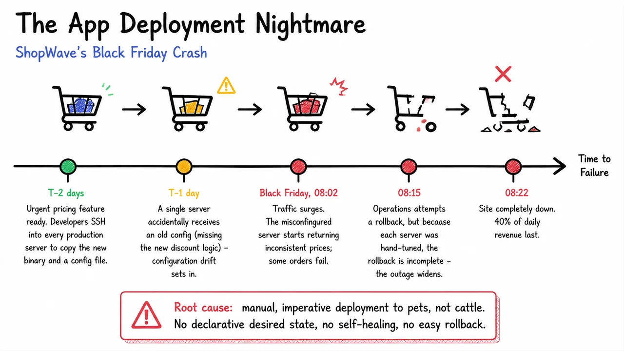
Consider a fictional but painfully familiar e‑commerce platform, ShopWave. Their engineering team had always treated production servers as pets—hand‑tuned, lovingly crafted, and irreplaceable. Each machine carried a unique history of patches, kernel tweaks, and application configs applied by different engineers over many months. A new pricing feature that had to ship before Black Friday was deployed the pet way: developers opened SSH sessions to every production node and manually deployed the updated binary and a new discount config file. The following 72 hours exposed every flaw in that model.
The timeline is instructive. Two days before Black Friday (T‑2), the manual push began. With no automated validation, the team had no way to verify that every server received the correct config. The next day (T‑1), an operations engineer discovered that one machine had been given an old config file, missing the critical discount logic. However, without a central source of truth, there was no quick way to identify which other servers might be similarly tainted. The drift was real, but incomplete; some parts of the fleet were already broken. At 08:02 on Black Friday, traffic surged. The misconfigured server began returning inconsistent prices, causing some orders to fail silently. By 08:15, the operations team initiated a rollback. But because each server’s state had been uniquely hand‑tuned, the rollback was a partial patchwork—some nodes reverted correctly, others didn’t, and a few received yet another unintended config version. The outage widened. At 08:22 the entire site went dark. The financial hit was staggering: an estimated 40% of daily revenue evaporated in minutes.
This nightmare has a clear root cause: manual, imperative deployment to pets, not cattle. In the cattle, not pets metaphor, servers are disposable and indistinguishable. If one misbehaves, you replace it, not nurse it back to health. A declarative approach codifies the desired state of each component—the exact container image, the exact resource limits, the exact networking policy—and a control loop continuously reconciles the actual cluster state with that declaration. When a server drifts or dies, the orchestrator spots the discrepancy and heals it automatically. Rollbacks become trivial: you simply change the declared state to a previous known‑good version, and the system ensures convergence. Self‑healing, version‑controlled declarative configurations, and automated health checks transform a fragile artisanal setup into a resilient, scalable platform.
The visual below encapsulates this cascade in a compact timeline that distills the sequence of events—from the initial hurried deployments through silent configuration drift to the accelerating failure on Black Friday—into a single glance. The hand‑drawn markers, shifting from green (hope) through yellow (warning) to red (catastrophe), trace the “time to failure” that manual processes guarantee. A stylised shopping cart icon fracturing above the timeline reinforces the business impact: revenue literally breaking apart as the system unravels. The callout box anchoring the root cause—manual imperatives, no self‑healing—ties the story back to the central lesson. More than a cautionary tale, the timeline becomes a concise argument for why Kubernetes and other orchestrators exist: to replace this fragile, imperative patchwork with a declarative, self‑correcting system that can survive the Black Fridays of the real world.
2. Kubernetes at a Glance
After witnessing the chaos of bespoke shell scripts, config drift, and manual recovery procedures, the natural question is whether there exists a unifying abstraction that can tame the complexity of containerized workloads. That abstraction is Kubernetes, an open‑source platform built on a single, powerful idea: declare the desired state of your application, and let the system continuously drive reality toward that declaration.
The Kubernetes programming model is inherently declarative. Instead of scripting a sequence of “start three containers, watch them, restart if failed, add a load balancer…”, you provide a desired state – for example, “I want three replicas of a web server, each listening on port 8080, with a network identity that balances traffic across them.” You submit this intent as a YAML or JSON resource (a Deployment, in this case) to the cluster. Kubernetes does not ask how you arrived at this state; it simply agrees to make the world look like the specification, and to keep it looking that way indefinitely.
The engine that makes this possible is a distributed control loop running across the cluster. Conceptually, the loop is simple: observe the actual state of the system, compare it with the desired state, and perform the minimal set of actions needed to eliminate any gap. This cycle repeats continuously, not on a timer triggered by user action, but as an eternal background process. If a node fails and a container disappears, the observed state diverges; the control loop immediately schedules a replacement on a healthy node, restoring the desired replica count. This self‑healing behavior is not a special feature bolted on later – it is a direct consequence of declarative reconciliation.
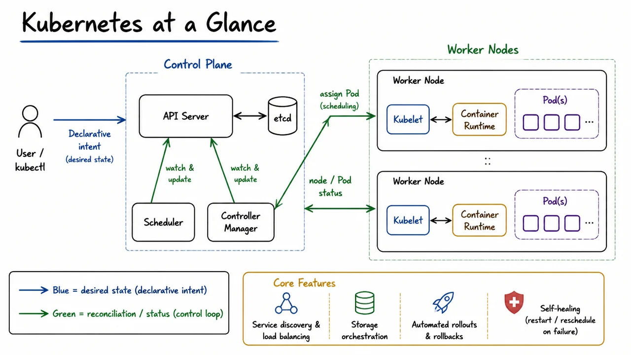
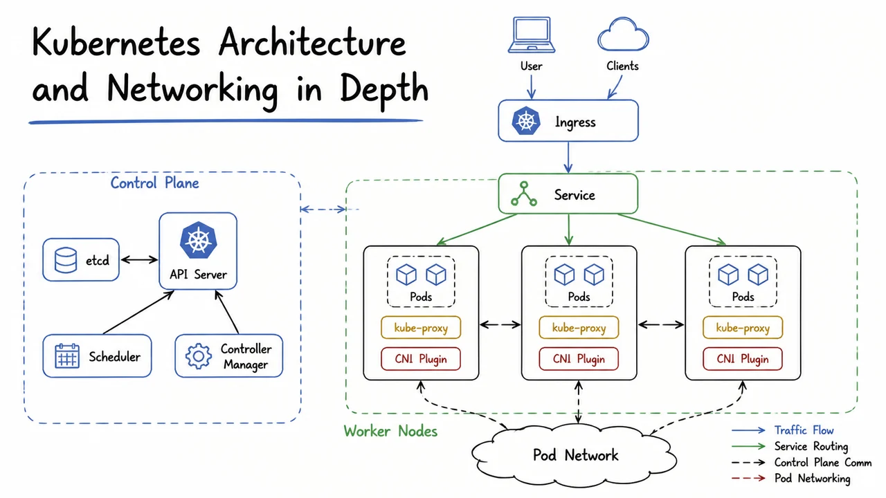
To realize this loop, Kubernetes partitions the cluster into two distinct planes: the control plane and a set of worker nodes. The control plane stores desired state, makes scheduling decisions, and orchestrates all reconciliation steps, while worker nodes simply run application containers and report their status back. The front door to the control plane is the API Server, a RESTful hub through which every request – whether from a user, an internal component, or an external automation – passes. No other component communicates directly with etcd; all reads and writes go through the API Server, providing a strong audit boundary and a consistent point of authorization.
Behind the API Server, etcd acts as the cluster’s source of truth, a distributed key‑value store that holds both the desired state (e.g., Deployment manifests) and the observed state (e.g., which Pods exist, their IP addresses, health status). Tightly coupled to the API Server are two control-plane processes that watch for changes and act autonomously. The Scheduler monitors for Pods that have been created but not yet assigned to any worker node; when it finds such a Pod, it evaluates node resource availability, affinity rules, and taints/tolerations, then writes the chosen node name back into the Pod’s specification via the API Server. The Controller Manager runs a collection of dedicated controllers, each responsible for a particular resource type (ReplicaSet, Deployment, EndpointSlice, and many others). Each controller watches its own subset of resources and continuously drives the cluster toward the declared intent – for example, the ReplicaSet controller creates or deletes Pods to match the desired replica count.
On the worker‑node side, the kubelet is the agent that bridges the control plane to the container runtime. The kubelet watches the API Server for Pods assigned to its node, pulls any necessary container images, and calls the local Container Runtime (such as containerd or CRI‑O) to start and manage the containers. It then reports container and node health back to the API Server, closing the reconciliation feedback loop. A single Pod, drawn as a logical envelope around one or more tightly coupled containers, is the atomic unit of scheduling and scaling – all containers in a Pod share the same network namespace, IP address, and storage volumes, which radically simplifies co‑located helper processes like log shippers or sidecar proxies.
The interplay between these components crystallizes into a clean architectural pattern: the user expresses intend (“run three web server replicas”) and the control plane – through the API Server, Scheduler, Controller Manager, and etcd – determines where and how to place Pods, while worker nodes execute the actual containers and report status. This separation of declarative intent from imperative execution is the key insight that makes Kubernetes resilient, extensible, and ultimately manageable at scale.
The diagram below distills this high‑level flow into a visual narrative that is easy to recall. On the left side, the Control Plane groups the API Server, etcd, Scheduler, and Controller Manager. A user icon labeled User / kubectl sends a blue arrow of declarative intent to the API Server, mirroring how a kubectl apply command carries a desired‑state specification. Green arrows trace the reconciliation heartbeat: the Scheduler and Controller Manager watch the API Server and write back decisions, while worker‑node agents push Pod and node status upstream. A bidirectional connection between API Server and etcd underscores that all persistent state flows through the API Server. On the right, each Worker Node contains a kubelet and Container Runtime, with Pods drawn as container groups, emphasizing that the node’s role is execution and status reporting. The legend – blue for “desired state”, green for “reconciliation / status” – makes the separation of concerns immediately legible, reinforcing that Kubernetes’ core loop is not a clever add‑on, but the very architecture of the system.
3. Monolith to Microservices: A Concrete Failure Case
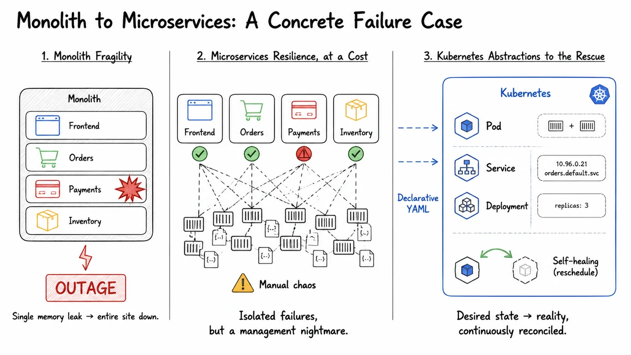
When a monolith falls, it falls all at once. The previous section gave a high‑level glance at Kubernetes, but the true value of orchestration only crystallizes when you’ve experienced the fragility that it was designed to eliminate. Imagine a typical e‑commerce application running as a single deployable artifact: the frontend, order processing, payments, and inventory management are all welded together into one process. This tight coupling makes development and initial deployment simple, but it carries a catastrophic failure mode. A single memory leak inside the payment module—perhaps a misconfigured cache that never evicts entries—doesn’t stay contained. It starves the entire process of memory, causing every other functional area to crash along with it. The whole site goes dark. And when the pressure mounts during a flash sale, scaling means replicating the entire stack, not just the bottleneck component. That is both expensive and slow: you are provisioning full replicas of frontend code, database connections, and session caches just to absorb a spike in payment volume.
Moving to microservices addresses this fragility by splitting the monolith into independently deployable units. Each component—frontend, orders, payments, inventory—runs in its own process, often in its own container. A memory leak in the payment service now only brings down payments; the frontend continues rendering pages (perhaps showing a graceful “payment unavailable” message), orders can still be viewed, and inventory updates proceed unaffected. This blast‑radius containment is a dramatic improvement. The trouble is that resilience doesn’t come for free. You’ve traded one monolithic process for dozens of small, interconnected containers, each with its own resource limits, health checks, inter‑service networking, configuration secrets, and versioned image lifecycles. Without automation, the operational burden becomes overwhelming. Manually starting containers, keeping their IP addresses straight, wiring up load balancers, and rolling out updates turns into a brittle, error‑prone chore. Often, teams end up with a messy cluster of script‑driven container restarts and hand‑written configuration files that works only under the watchful eye of the person who built it—a classic manual chaos state.
This is precisely the gap Kubernetes fills, and it does so with a handful of strongly‑typed abstractions that codify the patterns engineers were otherwise re‑inventing by hand. The Pod is the atomic unit of scheduling and scaling: a co‑located group of containers that share a network namespace and storage volumes. It represents the smallest “deployable unit,” not an individual container. By grouping sidecars alongside main containers (say, a log shipper next to an application), Kubernetes preserves the local communication guarantees that microservices often rely on. Next, the Service solves the ephemeral‑nature problem. Pods come and go; their IP addresses change. A Service provides a stable virtual IP and DNS name that load balances across a dynamic set of Pods matching a label selector. This decouples how clients find a service from which Pod instances are currently healthy, a prerequisite for both scaling and rolling updates. Finally, the Deployment is the declarative controller that takes a desired state—for example, “I want three replicas of the orders container image orders:v2”—and continuously reconciles reality with that specification. It rolls out new versions with zero‑downtime strategies, monitors Pod health, and replaces failed instances automatically.
These three abstractions turn the manual nightmare into an automated, self‑healing system. Instead of a human operator reacting to a crash by ssh‑ing into a host and restarting a container, a Deployment simply observes that a Pod is missing and spins up a new one. Instead of reconfiguring load balancers every time a backend scales, the Service transparently routes traffic only to Pods bearing the right labels and passing readiness checks. The operator’s job shifts from procedure to policy: they express intent in a handful of lines of YAML, and Kubernetes handles the rest. That’s a monumental shift in reliability and developer velocity.
The visual below condenses this entire journey into a side‑by‑side comparison that acts as a mnemonic for the trade‑offs. On the left, a monolithic block encloses all components; a red explosion overlays the payments box and a jagged arrow points to an “OUTAGE” banner—one leak collapses everything, and scaling requires replicating the whole block. In the centre, four independent microservices are shown, with payments flagged in red and the others green, illustrating isolated failures. But below them sits a tangled mess of container rectangles and configuration files, guarded by a yellow warning sign: the manual chaos that makes microservices unmanageable at scale without help. Finally, on the right, a large Kubernetes box wraps icons for Pod, Service, and Deployment, with a green self‑healing loop restarting a failed Pod. Faint arrows flow from the microservices chaos into the Kubernetes realm, labeled “Declarative YAML,” making it explicit that Kubernetes is not a new architectural style but a platform that transforms the messy reality of microservices into a continuously reconciled desired state. The diagram thus captures the core insight: microservices give you resilience, but only Kubernetes (or a similar orchestrator) makes that resilience operationally tenable.
4. The Control Plane
The chaotic manual scaling and recovery attempts we explored in the previous section all share a common failure mode: there is no agent that persistently watches the entire system and enforces a declared intention. Kubernetes addresses this by placing a dedicated set of coordinating components at the heart of every cluster. Together, these components form the control plane—the brain that accepts your desired state, stores it durably, and continuously reconciles the actual state of your workloads with that specification.
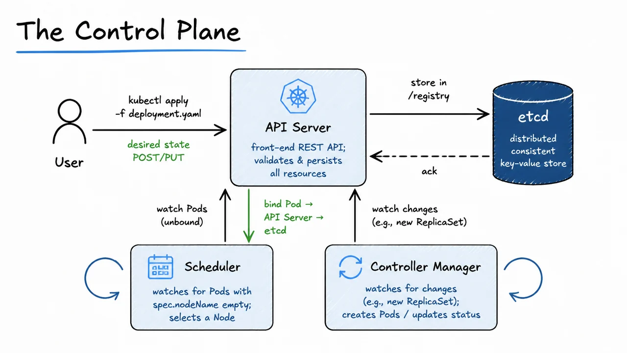
All operations inside the control plane flow through a single entry point: the API Server. This is a RESTful front-end that validates, authenticates, and marshals every resource definition—Pods, Services, Deployments, ConfigMaps, and everything else—into a canonical representation. The API Server exposes endpoints for both human operators (via kubectl) and internal components, but it never initiates work on its own. Its role is to gate, persist, and distribute information. Every mutating request is checked against the cluster’s Role-Based Access Control (RBAC) rules and admission controllers before being accepted, ensuring that no component can violate the cluster’s security or consistency guarantees.
The persistent record of all accepted state lives in etcd, a distributed, strongly consistent key‑value store. etcd uses the Raft consensus algorithm to replicate data across multiple control‑plane nodes, so the loss of a single machine does not destroy the source of truth. Crucially, etcd is a passive store: no other control‑plane component ever writes to it directly. The API Server is the sole writer, which means every change to cluster state—whether a new Pod definition, a node heartbeat, or an updated Deployment replica count—is auditable and uniformly serialised. The store is typically organised under a directory‑like key structure (e.g., /registry/deployments/<name>) that mirrors the Kubernetes resource model.
Two main actors consume this state to make the cluster do real work: the Scheduler and the Controller Manager. The Scheduler watches the API Server for Pods that have been created but not yet assigned to any Node—identified by a missing spec.nodeName field. For each such Pod, it evaluates every eligible Node by filtering out those that lack sufficient resources, violate affinity or anti‑affinity rules, or are tainted. It then scores the remaining candidates using a configurable set of priorities (e.g., spreading Pods across failure domains, bin‑packing for efficiency) and picks the best fit. The decision is not applied directly to etcd; instead, the Scheduler sends a “binding” request back to the API Server, which updates the Pod’s node assignment and persists the change. This feedback loop keeps all decisions auditable and retryable.
The Controller Manager houses a collection of independent control loops, each responsible for a specific resource type. Although they are often drawn as a single box, they are logically separate processes that share the same binary for operational convenience. The ReplicaSet controller, for example, continually compares the number of healthy Pods that match a ReplicaSet’s selector against the desired replicas; if a Pod dies, it creates a replacement Pod definition via the API Server. The Deployment controller builds on top of ReplicaSets to orchestrate rolling updates and rollbacks. The Node controller monitors the health of cluster nodes and, after a timeout, marks them as unavailable and evicts their Pods. The Endpoints controller tracks which Pods belong to a Service and updates the corresponding Endpoints object whenever Pods come and go. All these controllers operate by the same reconciliation loop pattern: observe current state through the API Server, compare it with the desired state stored in etcd, and issue create/update/delete requests to drive the two into alignment.
This watch‑driven design means that the control plane does not push commands to Node components like a traditional orchestrator. Instead, every agent pulls the state that concerns it. A typical lifecycle for a user‑submitted Deployment illustrates the chain of events. A developer runs kubectl apply -f deployment.yaml. The CLI sends an authenticated HTTP request to the API Server containing the Deployment object. The API Server validates the schema, calls admission plugins, and—if all checks pass—writes the object to etcd under /registry/deployments/<name>. An acknowledgment flows back to the user. At this moment, no Pods or ReplicaSets exist; only the declaration lives in etcd.
Now the Controller Manager’s Deployment controller, which has been long‑polling for new Deployment events on the API Server, picks up the write. It reads the Deployment’s replicas and Pod template, constructs a ReplicaSet specification, and sends a create request to the API Server. Similarly, the ReplicaSet controller observes the newly created ReplicaSet, computes the required number of Pods, and submits Pod definitions to the API Server—each with an empty spec.nodeName. The Scheduler, watching for unscheduled Pods, sees this batch. It scores all feasible Nodes, binds each Pod to the selected Node via a separate API call, and the assignments land in etcd. Only then does the kubelet on the chosen Node pull the container images and start the containers. At every step, the sole writer to etcd is the API Server, and all participants act as clients that observe and mutate state through that single interface.
The visual below turns this narrative into a traceable diagram that makes the hub‑and‑spoke topology immediately apparent. The user initiates the flow on the left, the API Server sits in the centre as the sole mediator, and etcd on the right persists everything with a dark‑blue shading that distinguishes it from the light‑blue computation components. The Scheduler and Controller Manager are shown as passive watchers with looping arrows, reinforcing that they do not receive direct commands but instead react to changes they poll from the API Server. Specific labels—“desired state POST/PUT”, “store in /registry”, and “bind Pod → API Server → etcd”—tightly map to the lifecycle of a Deployment you just walked through. The dashed acknowledgment from etcd back to the API Server underscores the store’s role as a durable, consensus‑backed source of truth, not an active participant. Together, these elements compress a complex asynchronous reconciliation engine into a single glance‑and‑you‑get‑it Excalidraw piece, serving as both a learning aid and a mental model for reasoning about Kubernetes control‑plane interactions.
5. Node Components
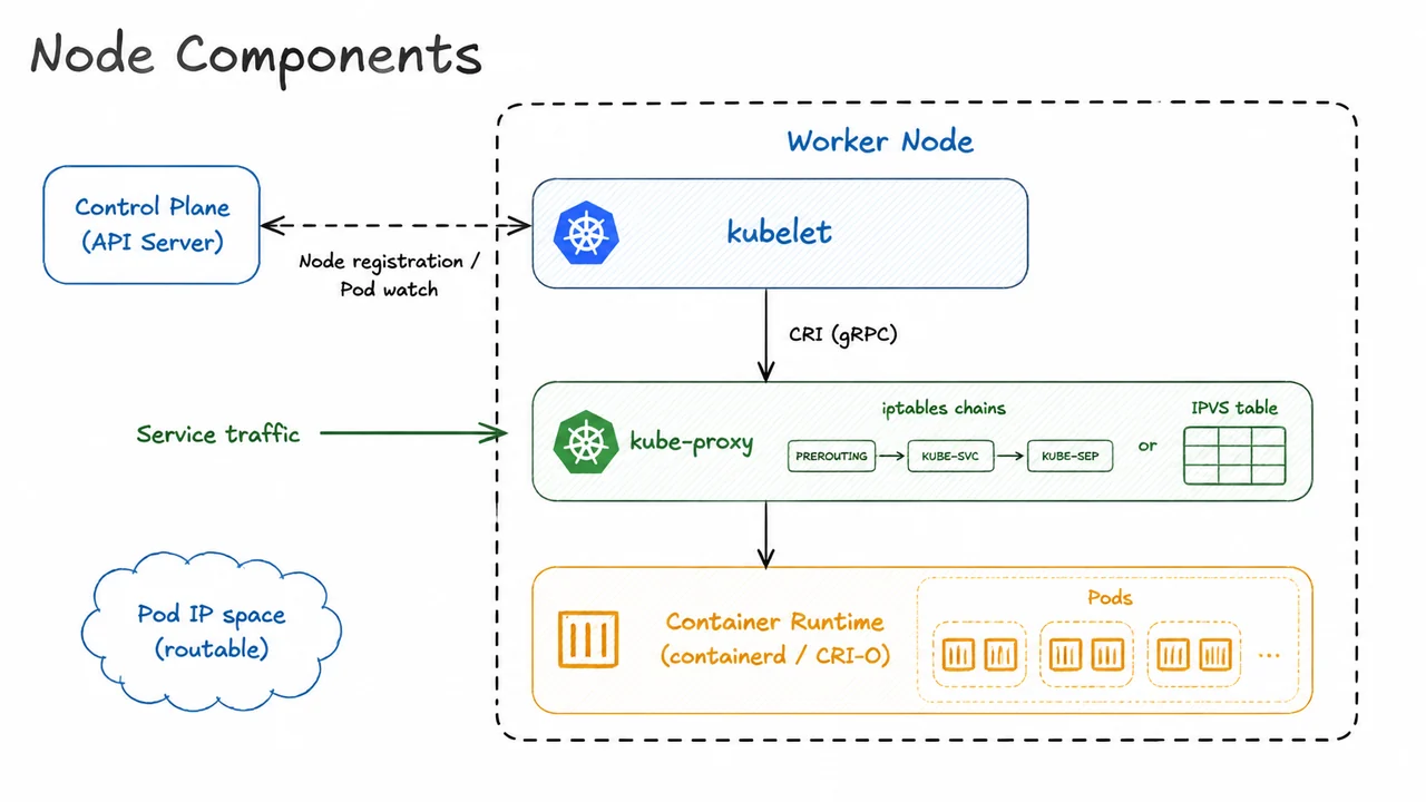
Having explored the brain of the cluster—the control plane’s API server, scheduler, controllers, and etcd—we now descend to the muscle. The worker nodes are the machines where Kubernetes actually runs your containers, and every node relies on a trio of co‑operating agents that turn declarative intent into executing workloads. These three components, the kubelet, kube‑proxy, and the container runtime, each handle a distinct layer of the node’s responsibility, and their interplay is what makes a node a full‑fledged Kubernetes citizen.
At the heart of the node sits the kubelet. It is not a container itself but a systemd service (or equivalent) that acts as the node’s representative to the control plane. When a node joins the cluster, the kubelet registers it by creating a Node object in the API server. From that moment on, the kubelet continuously watches the API server for Pods that have been assigned to its node—specifically, Pods whose spec.nodeName field matches the node’s name. When a new Pod appears, the kubelet does not directly launch processes. Instead, it calls down to the container runtime through a well‑defined gRPC‑based interface: the Container Runtime Interface (CRI). This indirection is crucial; it allows Kubernetes to support multiple runtimes (containerd, CRI‑O, and others) without changing the kubelet. The CRI operations map neatly to Pod‑level verbs—RunPodSandbox, CreateContainer, StartContainer—so that the kubelet can orchestrate the entire lifecycle of a Pod and its containers. The kubelet also runs periodic health checks (liveness and readiness probes), reports node and Pod statuses back to the API server, and manages volumes and secrets on the node’s filesystem.
If the kubelet is the node’s brain stem, then kube‑proxy is its networking switchboard. The Service abstraction in Kubernetes provides a stable virtual IP and DNS name for a set of Pods, but that abstraction must be materialised on every node so that traffic can reach the right backend. kube‑proxy runs on each node as a DaemonSet‑style process (or a static Pod) and watches the API server for Services and EndpointSlices (or Endpoints). It then programs the node’s kernel netfilter subsystem accordingly. Historically this meant writing iptables rules: every Service port mapping gets a chain of rules that randomly selects a backend Pod IP using a statistic module, effectively implementing a simple round‑robin load balancer. While iptables works, it scales poorly—the number of rules grows as , and rule updates can be slow. The modern alternative is IPVS (IP Virtual Server), which kube‑proxy can use in IPVS mode. IPVS creates kernel‑level virtual servers with configurable scheduling algorithms (round‑robin, least connections, source‑hash, etc.) and can handle thousands of Services with far lower latency and CPU overhead. Regardless of the backend, kube‑proxy ensures that when a container inside any Pod connects to a Service IP, the packets are transparently redirected to a healthy backend Pod.
The third agent, the container runtime, is the lowest‑level component. It is the software that actually pulls container images from registries, creates the OCI‑compatible container environment (namespaces, cgroups, root filesystem), and runs the application process. The runtime must implement the CRI to speak with the kubelet, but under the hood it typically relies on a lower‑level OCI runtime like runc to spawn the actual container. In practice, containerd and CRI‑O are the two dominant CRI runtimes. containerd is a general‑purpose container supervisor that can also serve Docker (though Docker itself is no longer the recommended Kubernetes runtime), while CRI‑O was purpose‑built for Kubernetes and keeps a minimal footprint. Both pull images according to the OCI image specification and manage container lifecycles. From the kubelet’s perspective, the runtime is a black box that obeys CRI calls; the runtime, in turn, enforces the node’s pod security context, mounts volumes, and attaches the container to the appropriate network namespace (usually via CNI plugins, which we will cover later).
These three agents do not operate in isolation; they form a tight vertical stack on every worker node. The kubelet registers the node and receives Pod specifications, then instructs the container runtime to materialise those Pods via CRI. kube‑proxy, watching the same API server independently, programs the node’s network rules so that Services can reach the Pods running on this node and others. The container runtime executes containers that exist inside that very networking fabric—each Pod gets its own routable IP address from the cluster’s Pod network, a flat IP space that must be reachable from any other Pod without NAT.
The visual below consolidates this architecture into a single diagrammatic slide. A large bounding box represents the worker node, and inside it three stacked blocks capture the agents: the kubelet at the top, kube‑proxy in the middle, and the container runtime at the bottom. A dashed arrow from the kubelet reaches out to an external “Control Plane (API Server)” box, labelled “Node registration / Pod watch,” emphasising the kubelet’s role as the node’s link to the cluster’s state. Another solid arrow descends from the kubelet into the container runtime, with the annotation “CRI (gRPC),” illustrating the clear interface contract. In the kube‑proxy block, we see it managing either a chain of iptables rule boxes or an IPVS table, with incoming traffic labelled “Service traffic” entering from the left—a whisper of the actual packet journey. The container runtime encloses small pod icons, reminding us that this is the execution sandbox where containers run, and the whole node is surrounded by a dashed boundary with the note “Pod IP space (routable)” to indicate that every Pod on the node participates in the cluster‑wide flat network. The diagram thus becomes a compact mnemonic for the symbiotic relationship between registration, workload scheduling, network service abstraction, and container execution that defines every Kubernetes worker node.
6. Pod: The Smallest Deployable Unit
Building on our understanding of the node’s internal machinery—the kubelet that babysits containers and the kube‑proxy that wires up network rules—we now turn to the fundamental unit that ties these components together: the Pod. While a node hosts many processes, the Pod is the atomic object that Kubernetes schedules, manages, and reasons about. It is simultaneously a deployment unit, a co‑location boundary, and a shared context bundle. Recognizing why this abstraction exists clarifies how Kubernetes scales without sacrificing the simplicity of single‑host development patterns.
A Pod is, in its simplest form, a collection of one or more containers that share a lifecycle, a network identity, and storage volumes. Crucially, all containers within a Pod are co‑located on the same node and are scheduled as a single, inseparable group. When the scheduler picks a node for a Pod, it does not place individual containers—it guarantees that the entire Pod’s containers will start on that same machine. This atomic scheduling eliminates the complexity of coordinating the placement of tightly coupled helpers like sidecars, adapters, or ambassadors. The kubelet, our agent on the node, then interprets the Pod spec and ensures every container in the Pod is running, restarting any that fail according to the Pod’s restart policy. In other words, the Pod is the smallest executable unit that Kubernetes directly manages, and all higher‑level abstractions—Deployments, StatefulSets, DaemonSets—ultimately orchestrate Pods.
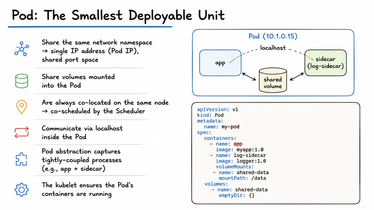
The most transformative property of a Pod is its shared network namespace. Every container inside a Pod sees the same Linux network stack: a single, unique IP address (the Pod IP), a shared localhost interface, and a common port space. This means containers can reach each other by simply addressing localhost and a port, exactly as if they were multiple processes on a single host. No makeshift registries, no external service discovery, no port remapping. For sidecar patterns—say, an application container that writes unstructured logs to a file while a fluentd sidecar ships them to a central store—the two containers can use localhost to exchange heartbeats or signals, and they can mount the same volume for log files. The network model also imposes a clean constraint: two containers in the same Pod cannot bind to the same port, which mirrors the behavior you’d expect from a single machine and prevents communication ambiguities.
Complementing the network identity, shared volumes provide the Pod’s storage context. A volume defined in the Pod spec can be mounted into one or more containers at independent mount paths. The simplest volume type, emptyDir, is created when the Pod is scheduled and destroyed when the Pod is removed—an ephemeral scratch space perfect for intra‑Pod data sharing. In the logging sidecar example, an emptyDir backed by the node’s local disk or memory allows the app to write logs and the sidecar to tail them, with no coupling beyond the volume’s name. The lifecycle of the volume follows the Pod, not any individual container, so restarts or failures of the main app don’t lose the accumulated data as long as the Pod persists.
The atomic scheduler also encourages a disciplined mental model. Because every Pod gets its own IP and can request its own resource limits, the scheduler treats Pods as the unit of resource allocation and bin‑packing on nodes. If two containers must be co‑located but have wildly different resource needs, bundling them in one Pod forces the scheduler to find a node that can satisfy both profiles simultaneously. This can be both a strength (guaranteeing locality) and a subtle trap: an oversized sidecar can starve a node of resources or cause eviction of the entire Pod. Understanding this trade‑off is essential when designing Pod boundaries; you should only place containers in the same Pod when they are tightly coupled in both function and resource scaling profile.
The Pod abstraction is also declarative: you describe the desired state, and Kubernetes controllers work to make reality match. A minimal YAML snippet—omitted here for brevity but shown in the visual below—specifies two containers (app and log‑sidecar) with a shared emptyDir volume. The apiVersion: v1 and kind: Pod fields mark this as a primitive, standalone object, though in practice you almost never create such bare Pods directly. Instead, you embed this Pod template inside a controller like a Deployment, which adds replication, self‑healing, and rolling update semantics. The raw Pod object remains the kernel that every higher‑level controller expands upon, which is why understanding its fields (especially spec.containers, spec.volumes, and the implicit networking contract) is foundational.
The accompanying diagram distills this knowledge into a compact, intuitive picture. On one side, the key properties are summarized in text, but the right side shows a rounded rectangle labelled with a Pod IP—say, 10.1.0.15—enclosing two smaller container boxes (app and sidecar). A shared volume icon sits between them, underscoring the storage context, while the single IP address and localhost arrow lines emphasize the unified network namespace. Beneath the diagram, a syntax‑highlighted YAML snippet of the two‑container Pod with a shared emptyDir volume reinforces the declarative definition. This visual encapsulates the core insight: a Pod is not merely a group of containers, but a co‑scheduled, co‑networked, co‑stored atomic entity that turns the Kubernetes cluster into a distributed operating system for containers.
7. Workload Controllers: Deployments, ReplicaSets & More
Pods are wonderful for packaging a single instance of an application, but they are, by design, fleeting. A Pod can die because its Node fails, because the kubelet evicts it under memory pressure, or simply because a rolling update needs to replace it with a newer version. If you deploy a raw Pod resource, that’s the end of the story: Kubernetes will not resurrect it, no matter how much you wish for three copies of your web server to stay running. This is why we need controllers — control loops that watch the current state of the cluster, compare it against a declared desired state, and take action to close the gap. In Kubernetes, workload controllers are the machines that turn the desire for a certain number of identical, replaceable Pods into reality.
The simplest of these is the ReplicaSet. Its single job is to guarantee that a specified number of replica Pods exist at all times. You write a ReplicaSet manifest that includes a Pod template (exactly the same Pod spec you saw in the previous section) and a replicas field. The controller then creates or deletes Pods to match that number. If a Pod crashes or is evicted, the ReplicaSet immediately spawns a new one with the same identity‑defining labels, so that the overall set of matching Pods never drops below the target count. Internally, ReplicaSets track ownership using a selector that matches the Pod’s labels, which is why label management is so critical: the controller will adopt any Pod whose labels fall within its selector, even one it didn’t create, as long as it doesn’t have an existing owner reference. This label‑based ownership is the key to how controllers remain loosely coupled yet accurate.
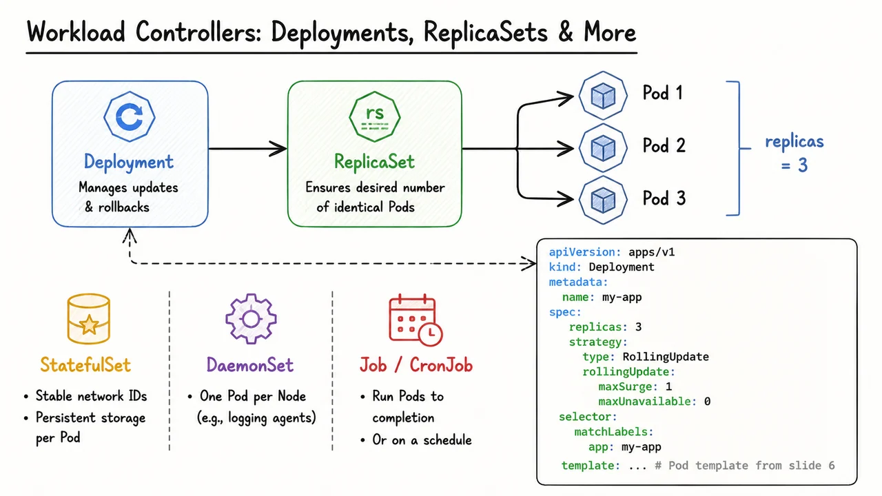
But you will rarely create a ReplicaSet directly. In production, you interact with a higher‑level abstraction: the Deployment. A Deployment wraps a ReplicaSet and adds lifecycle management on top of it. When you create a Deployment, it instantiates a ReplicaSet with the given Pod template and replica count. The real power comes when you change something in the Pod template — a new container image, an updated environment variable, a resource limit tweak. The Deployment does not mutate the existing ReplicaSet; instead, it creates a new ReplicaSet with the updated template and begins a rolling update. During the update, Pods from the old ReplicaSet are gradually scaled down while Pods from the new ReplicaSet are scaled up, maintaining availability according to the parameters you set.
The rolling update strategy is controlled by two fields: maxSurge and maxUnavailable. These are not percentages pulled from thin air — they define how many extra Pods may temporarily exist above the desired count (maxSurge) and how many Pods may be unavailable at any moment (maxUnavailable). For example, setting maxSurge: 1 and maxUnavailable: 0 with a replica count of three means the Deployment will create one new Pod first (bringing the total to four), wait for it to become ready, then terminate one old Pod, and repeat, ensuring that at least three Pods are always serving traffic. The Deployment also retains the old ReplicaSets (by default, the last ten) so that you can rollback instantly if the new version is broken. A single kubectl rollout undo command reverts the Deployment to the previous ReplicaSet, undoing the update with the same graceful rolling logic.
The declarative YAML for a Deployment ties everything together. You specify the kind: Deployment, set the replicas count, declare the rolling update strategy, and embed the Pod template under spec.template. The Deployment’s selector must match the labels in that template. Under the hood, the Deployment controller manages one active ReplicaSet and possibly several retired ones, while the ReplicaSet controller manages the actual Pods. This layered design gives you a clear separation of concerns: the Deployment handles versioning and rollout mechanics, the ReplicaSet handles sheer replica maintenance, and the Pod itself remains the atomic workload.
Beyond Deployments, Kubernetes provides other controllers for different workload patterns. A StatefulSet is used when Pods need stable, unique network identities (like web-0, web-1, …) and persistent storage that survives Pod rescheduling. A DaemonSet ensures that exactly one Pod runs on every Node (or a subset), ideal for log collectors, monitoring agents, or node‑local caches. For batch workloads, a Job creates one or more Pods and ensures they all run to completion, while a CronJob spawns Jobs on a time‑based schedule. Each of these controllers ultimately manages Pods using the same core control loop pattern, but they expose a different mental model to the cluster operator.
The visual below consolidates this hierarchy and these relationships in a single diagram that functions much like a mental map. At the top, a Deployment box feeds into a ReplicaSet box, which in turn fans out to three Pod icons — an immediate reminder that the Deployment you define in YAML ultimately expresses itself as a set of running Pods, but never directly. The Deployment YAML snippet on the right, connected by a dashed arrow back to the Deployment box, reinforces that the text you write is the input to the top‑level controller. Meanwhile, three columns below summarize the other controller types — StatefulSet, DaemonSet, and Job/CronJob — each with a tiny iconic cue and a one‑liner of its purpose, so you can quickly map a workload requirement to the right controller without wading through paragraphs of text.
8. Services: Stable Network Identity for Ephemeral Pods
Pods are the atomic schedulable units in Kubernetes, but they are volatile by design. A Deployment ensures that a desired number of replicas are running, and a ReplicaSet continuously brings new Pods to life when old ones fail or are evicted. Each of those Pods receives its own IP address from the cluster’s pod network. That address is ephemeral—it changes whenever the Pod is rescheduled or restarted. Relying on individual Pod IPs for inter‑service communication would force every client to discover and track a shifting list of endpoints, which is brittle and antithetical to the loose coupling that cloud‑native systems strive for.
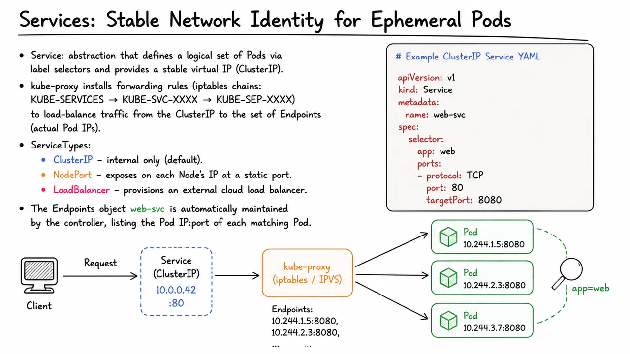
This is exactly the tension that the Service abstraction resolves. A Service defines a logical grouping of Pods through a label selector and gives that set a stable network identity: a virtual IP address called the ClusterIP. Clients inside the cluster talk to the ClusterIP, unaware of which concrete Pods are currently backing the service. The Service itself never restarts; its ClusterIP persists for the lifetime of the resource, providing a reliable handle for load‑balanced traffic.
The magic that turns a virtual IP into concrete packets destined for a real Pod is performed by a component running on every node: kube‑proxy. In its default iptables mode, kube‑proxy watches the API server for Services and Endpoints objects and programs iptables rules on the local node. When a packet arrives at the node with the ClusterIP as its destination, the rules rewrite the destination address (DNAT) to the IP of one of the healthy backend Pods. The decision is a simple form of load balancing: each rule chain statistically distributes traffic according to a random selection over the available Endpoints.
The iptables rule hierarchy follows a predictable pattern. A chain named KUBE-SERVICES catches any packet whose destination matches a ClusterIP. That chain jumps to a per‑Service chain, typically KUBE-SVC-XXXX, which handles the port mapping from the Service’s external port to the Pod’s targetPort. From there the traffic is dispatched to individual KUBE-SEP-XXXX chains—one per Endpoint—where the final DNAT to that specific Pod IP and port occurs. The entire sequence is stateless and distributed: every node runs its own copy of these rules, so any node can forward traffic for any Service, regardless of where the backend Pods are located.
Three common ServiceTypes control how the Service is reachable from outside the cluster:
- ClusterIP (the default) exposes the Service only on an internal virtual IP, accessible solely from within the cluster.
- NodePort builds on ClusterIP and opens a static port (
30000‑32767by default) on every node’s primary network interface. External traffic hitting<NodeIP>:<NodePort>is forwarded to the ClusterIP, giving simple external access without a cloud load balancer. - LoadBalancer extends NodePort and, in cloud environments, provisions an external load balancer (such as an AWS ELB or GCP forwarding rule) that directs traffic to the NodePort on each node, effectively giving you a public, stable IP or hostname.
A typical ClusterIP Service is declared with a minimal YAML descriptor:
apiVersion: v1
kind: Service
metadata:
  name: web-svc
spec:
  selector:
    app: web
  ports:
    - protocol: TCP
      port: 80
      targetPort: 8080
Here the selector app: web ties this Service to every Pod that carries that label. Incoming traffic on port 80 of the ClusterIP is forwarded to port 8080 on the selected Pods. The Service’s own name, web-svc, is resolvable via cluster DNS, so clients can connect to http://web-svc without ever knowing the ClusterIP itself.
Behind the scenes, the Service controller automatically maintains an Endpoints object named web-svc. This object is essentially a list of IP:port pairs—one for each Pod that currently matches the label selector and has passed its readiness probes. As Pods are created, destroyed, or change their label, the Endpoints object is updated instantly. kube‑proxy subscribes to these changes and adjusts iptables rules (or, in IPVS mode, the kernel’s IP Virtual Server tables) to reflect the new set of healthy backends. This tight feedback loop keeps the traffic flowing to the right Pods without any manual intervention, even during rolling updates or node failures.
The visual that follows brings these pieces together in a single coherent picture. It illustrates a client’s request traveling to a stable ClusterIP—shown as a distinct virtual address—and then being intercepted by kube‑proxy’s forwarding logic, which fans the request out to one of several concrete Pods, each with its own dynamic Pod IP. The label selector is depicted as a magnifying glass drawing a dashed connection between the Service and the matching Pod set, emphasizing that membership is dynamic and declarative. Surrounding the core flow, three color‑coded callouts represent the ClusterIP, NodePort, and LoadBalancer exposure modes, reminding the reader that the same internal load‑balancing mechanism underpins every way a Service can be reached. The compact YAML snippet on the right anchors the abstract diagram in a real configuration, making the mapping from spec fields to runtime behavior tangible.
9. Kubernetes Networking Model & CNI
After exploring how Services provide a stable entry point for ephemeral Pods, we need to examine the network substrate that makes such abstractions both possible and predictable. Services, load‑balancing, and Ingress all rely on a lower‑level guarantee: that every Pod in the cluster can be addressed directly by its own IP, from any other Pod or node, without the aid of port mapping or network address translation. This guarantee is not a happy accident of container orchestration—it is a deliberate design choice codified in the Kubernetes networking model. Understanding that model, and the plug‑in machinery that implements it, is essential before we can reason about more advanced topics like network policy or CNI selection.
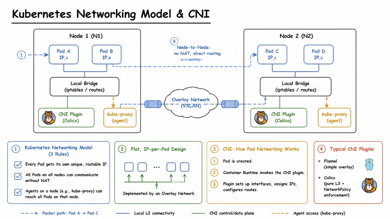
The Kubernetes networking model rests on three fundamental requirements that every conformant cluster must satisfy. First, each Pod receives its own unique, routable IP address—IP‑per‑Pod. Second, all Pods on a node can communicate with all Pods on all other nodes without NAT; cross‑node Pod traffic must be treated as native, un‑masqueraded IP communication. Third, system agents on a node (such as the kubelet and kube‑proxy) must be able to reach all Pods running on that same node using their Pod IPs. These are not optional features; they are the irreducible contract that allows Kubernetes to treat Pods as “virtual hosts” that share the same network namespace within a Pod but are isolated from the outside world only by the rules we explicitly define.
Notice what this model intentionally excludes: there are no NAT gateways between Pods, even when they reside on different subnets or physical hosts. This stands in stark contrast to the default bridged network in Docker, where a container’s IP is hidden behind a host‑internal bridge and outbound traffic hides behind the host’s external address. Kubernetes rejects that pattern because it would break fundamental assumptions: that a Pod’s identity is stable across restarts (its IP is not, but the address itself is directly meaningful), that service mesh sidecars can intercept traffic transparently, that network policies can enforce rules based on Pod labels and IPs without confusing address rewriting, and that kube‑proxy can program iptables rules that forward Service traffic directly to Pod IPs. In other words, the flat, IP‑per‑Pod network is the bedrock on which service discovery, policy, and security are built.
The word “flat” deserves a little nuance. It does not mean all Pods are on the same L2 broadcast domain; rather, it means the IP space behaves as though it were a single, routable address family spanning all nodes. Typically, a cluster‑wide CIDR block (e.g., 10.0.0.0/14) is divided into smaller per‑node subnets. When a node joins the cluster, it receives a subnet allocation, and the network plugin ensures that any Pod scheduled on that node gets an IP from that node’s subnet and that routes exist for the rest of the cluster to reach that subnet. This design elegantly avoids IP address conflicts and simplifies routing: a packet destined for 10.0.1.5 might belong to node1’s subnet, so the rest of the cluster simply routes traffic toward node1, where the local plugin knows exactly which Pod interface to deliver it to.
Implementing this model across arbitrary infrastructure—bare‑metal, virtual machines, different cloud providers—would be an integration nightmare if every environment required bespoke wiring. Here the Container Network Interface (CNI) enters as a crucial abstraction. CNI is a specification that defines how container runtimes interact with network plugins at the moment of Pod lifecycle events—primarily creation and deletion. The runtime (e.g., containerd, CRI‑O) does not need to know whether it is configuring a VXLAN tunnel, routing BGP, or applying an AWS VPC policy; it simply invokes the configured CNI binary with a standard JSON configuration, passing a container’s network namespace, and expects the plugin to set up interfaces, assign IPs, and plumb the necessary routes. This separation of concerns is what allows Kubernetes to remain infrastructure‑agnostic while the network ecosystem flourishes.
When a Pod is created, the flow is remarkably consistent across CNI implementations. The kubelet, via the Container Runtime Interface, calls the configured CNI plugin with parameters that include the Pod’s network namespace. The plugin’s responsibilities are threefold: allocate an IP address for the Pod from the node’s subnet or a global pool, create a veth pair (one end inside the Pod’s namespace, usually named eth0, the other on the host attached to a bridge or routed interface), and install routes on the host so that traffic to that Pod’s IP is directed to the correct virtual interface. Optionally, the plugin may also set up more elaborate data‑plane paths—setting up an overlay encapsulation, programming OpenFlow rules, or injecting iptables entries for network policy.
The landscape of CNI plugins is deliberately diverse, offering a range of trade‑offs between simplicity, performance, and policy capabilities. Flannel is perhaps the simplest overlay: it creates a VXLAN or UDP tunnel mesh between nodes, wrapping Pod traffic in an outer IP header that can traverse the physical underlay. This yields a flat network with minimal configuration burden but at the cost of per‑packet encapsulation overhead and limited policy enforcement. Calico takes a different approach: it treats Pod IPs as pure L3 endpoints and often runs a BGP daemon on each node to exchange routing information with the rest of the cluster (or even with physical routers). Because Calico operates at the routing layer without encapsulation (or with optional cross‑subnet IP‑in‑IP), it can be faster and integrates natively with standard network tools; it also pioneered tight integration with Kubernetes NetworkPolicy objects, enforcing them directly in the Linux kernel’s routing tables and iptables rules. Other plugins like Cilium rely on eBPF to push fine‑grained security and observability into the kernel, while Weave Net uses its own gossip‑based routing. All of them, however, satisfy the same CNI contract, ensuring that an ADD command hands back a working Pod IP that is reachable across the cluster without NAT.
With these components in mind, the diagram below synthesizes how the pieces fit together for a typical cross‑node communication scenario. Two nodes, each hosting a pair of Pods with unique IPs, illustrate the flat model’s promise: no NAT, no port remapping, just direct IP reachability. Inside each node, the CNI plugin (represented here by a Calico‑style component) manages the local bridge or route that connects the Pod’s eth0 to the host’s network stack. When Pod A on Node 1 wants to talk to Pod C on Node 2, the packet leaves Pod A’s interface, hits the local bridge, and is handed to the CNI data plane. In an overlay‑based setup (like Flannel or Calico with VXLAN), the CNI encapsulates the original packet and sends it across the physical underlay to Node 2, where the peer CNI instance decapsulates it and delivers the original packet to Pod C’s bridge and finally to the target Pod. The dashed arrow in the visual traces this exact path, while the label “Node‑to‑Node: no NAT, direct routing via overlay” reinforces that, from the Pods’ perspective, the connection is a pure IP exchange—they remain blissfully unaware of the encapsulation that spliced the two segments together. This encapsulation detail is the implementation secret that turns a heterogeneous set of physical networks into the single, flat IP space that Kubernetes promises.
10. CNI Plugins: Overlay Networks & Routing
The previous requirement—a flat, routable Pod IP space across every node—might be elegantly simple as a specification, but it says nothing about how packets actually travel from a Pod on one node to a Pod on another. That implementation is left entirely to the Container Network Interface (CNI) and the plugin you choose. Kubernetes does not ship a default overlay; instead, it delegates network setup to a CNI plugin that is invoked when a Pod is created or destroyed. The moment you install a cluster, you face a decision that will echo through every production debugging session and every latency-sensitive workload: which CNI plugin should I use? The answer balances simplicity, performance, NetworkPolicy support, and your tolerance for operational complexity.
At its core, a CNI plugin must provide IP connectivity for Pods while adhering to the Kubernetes networking model. But the “how” bifurcates into two broad families: overlay networks and pure L3 routing. Overlay networks encapsulate Pod traffic inside another protocol (usually VXLAN or another tunneling mechanism) so that the underlying physical network only sees host-to-host packets. This makes overlays incredibly portable—they work on any IP-capable underlay, regardless of topology—at the cost of encapsulation overhead and reduced observability. A pure routed approach, in contrast, injects Pod CIDRs into the host’s routing table and relies on standard IP forwarding, often augmented by BGP, to distribute routes across the cluster. The packets are never encapsulated; they travel natively across the fabric, yielding near line-rate performance but demanding that the underlay be capable of reaching those Pod IPs directly.
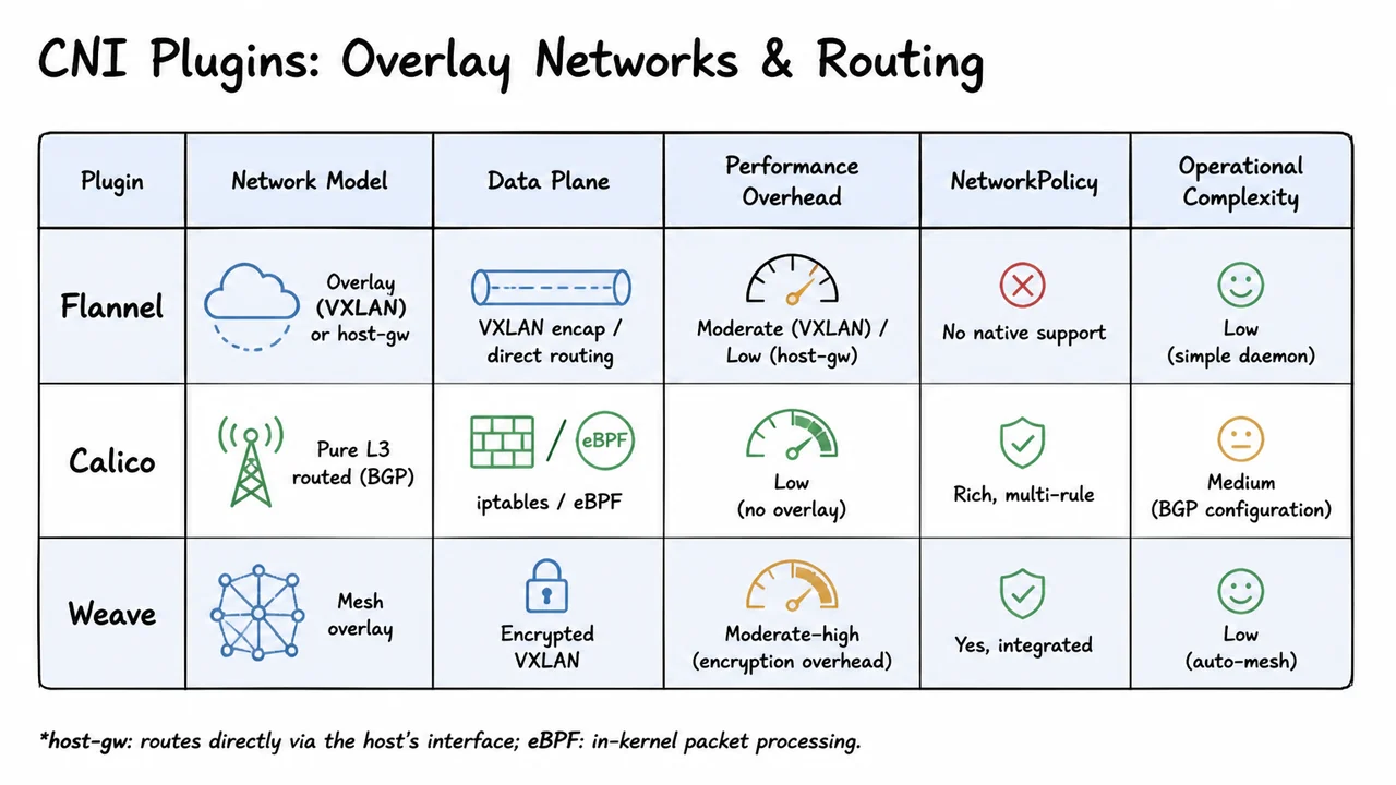
Flannel sits comfortably in the overlay camp, offering a dead‑simple daemon (flanneld) that allocates a per‑node subnet and uses VXLAN to bridge Pod traffic between nodes. There is almost no configuration; it “just works” on many environments, which explains its enduring popularity for development clusters and homelabs. Flannel also provides a host-gw backend that skips VXLAN entirely when all nodes are on the same L2 segment. In host-gw mode, Flannel simply programs the node’s routing table to reach remote Pod subnets via the next-hop node’s IP—pure L2 routing, no encapsulation, dramatically lower overhead. The trade-off is that host-gw requires direct L2 adjacency, breaking in any topology that crosses a router or requires an overlay. Crucially, Flannel offers no native NetworkPolicy support; if you need micro‑segmentation, you must layer another solution on top, which adds complexity that undermines Flannel’s simplicity.
Calico takes the opposite, L3‑routed path. It assigns each node a BGP AS number or uses a full mesh (or route reflectors) to propagate Pod prefix routes to every node’s routing table. The data plane can be either iptables (using Linux netfilter to enforce policy and perform basic forwarding) or eBPF programs that run directly in the kernel, bypassing the overhead of iptables’ linear rule chains. That architectural choice delivers consistently low latency and high throughput, because no encapsulation header is ever added. Calico also provides the richest NetworkPolicy model in the ecosystem, supporting global network policies, tiered rules, and extensive matching criteria far beyond the baseline Kubernetes API. The operational price is a medium learning curve: you must understand BGP peering, route reflectors, and cross‑subnet considerations, though Calico can also run in “overlay mode” using VXLAN if pure routing is infeasible.
Weave’s mesh overlay occupies a different niche: it builds a fully‑encrypted VXLAN mesh between every pair of nodes, using a gossip‑based protocol to distribute topology information. There is no central controller; every node participates and can route traffic. This auto‑mesh design makes Weave incredibly simple to deploy, often requiring only a single DaemonSet, and it provides transparent encryption for all Pod‑to‑Pod traffic out of the box—a property that is otherwise hard to guarantee without additional service mesh components. The overhead of encrypting every packet is non‑trivial, however, placing Weave in the moderate‑to‑high performance penalty category. Integrated NetworkPolicy support is present, but it is less expressive than Calico’s model. Weave’s strong suit is zero‑configuration security for clusters where ease of use trumps absolute throughput.
These divergent approaches create a palette of trade-offs that you can map onto your requirements. Performance‑sensitive workloads that can tolerate the loss of overlay encryption will gravitate toward Calico’s native routing or Flannel’s host-gw. Security‑first environments may accept the higher overhead of Weave’s mesh encryption or augment Calico’s policies with WireGuard. Simplicity‑minded teams often start with Flannel’s VXLAN and later migrate to Calico when NetworkPolicy becomes essential. The choice is not static; it is a decision you revisit as your cluster scales and as you layer on observability and security tools.
The comparison table that follows organizes these three plugins across six dimensions—network model, data plane, performance overhead, NetworkPolicy support, and operational complexity—giving you an at‑a‑glance reference for the trade-offs. The alternating row colors and bold plugin names make it easy to scan; small icons next to each model description (an overlay cloud for Flannel, a BGP radio tower for Calico, and a mesh net for Weave) reinforce the mental model. A footnote explains the host-gw and eBPF abbreviations that appear in the Data Plane column. Use this table as a decision aid when you are standing at the infamous CNI fork in the road, knowing that the implications ripple into every packet your cluster will ever carry.
11. kube-proxy Modes: userspace, iptables, IPVS
As we shift attention from the physical network fabric stitched together by CNI plugins to the logical service mesh, a crucial piece remains: how traffic destined for a stable ClusterIP actually finds a concrete Pod IP among a set of ephemeral backends. This is the responsibility of kube-proxy, a node-level daemon that bridges the Kubernetes API’s declarative abstractions with the kernel’s data plane. After CNI ensures any Pod can talk to any other Pod across nodes, kube-proxy ensures that clients targeting a Service do not have to track which Pods are alive, where they live, or what their exact IP addresses are at any given moment.
Kube-proxy continuously watches the API server for Service and Endpoints (or EndpointSlice) objects. When a Service is created or its backend Pods change, kube-proxy computes the load‑balancing decision for traffic arriving at the node on the Service’s ClusterIP and then programs that decision into the node’s operating‑system data plane. At its core, the process is a mapping from (ClusterIP:port) to a set of (PodIP:targetPort) tuples. The implementation, however, is not a single strategy; it comes in three distinct modes, each with its own data‑plane mechanism, scheduling algorithm, and scalability profile. Choosing the right mode can mean the difference between a cluster that hums along under heavy load and one whose network rules choke the kernel.
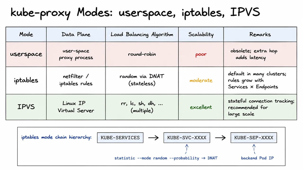
The userspace mode was the original design, now firmly obsolete. In this scheme, kube-proxy itself ran a user‑space TCP/UDP proxy. Traffic from the node’s network namespace was intercepted via iptables rules that redirected packets to a local port where the proxy process listened. The proxy then forwarded the connection to a selected backend Pod. Because packets had to cross the user–kernel boundary an extra time, userspace mode introduced significant latency and throughput bottlenecks. Its only load‑balancing algorithm was a simple round‑robin, and any failure of the proxy process meant lost connectivity. While historically important, you will not find it in modern, performance‑sensitive deployments.
Far more common today—and indeed the default in many clusters—is the iptables mode. Here, kube-proxy programs the Linux netfilter subsystem directly by inserting iptables rules. For each Service, it creates a chain hierarchy: KUBE-SERVICES catches incoming packets destined for a ClusterIP and dispatches them to a per‑Service chain KUBE-SVC-XXXX. That chain then uses the statistic match extension with --mode random and a --probability value to randomly DNAT the packet to one of the individual backend Pod rules in KUBE-SEP-XXXX chains. Because the selection is stateless—each packet independently undergoes a random draw—there is no load of connection tracking for load balancing decisions, but the probability weights are recomputed by kube-proxy when Endpoints change. The major drawback is that for every Service–Endpoint pair, a chain of rules must be created; thus the rule count grows as O(Services × Endpoints). On a node hosting hundreds of Services with many backends, the iptables rule list can balloon into tens of thousands of entries, slowing down rule synchronization and packet matching.
The recommended mode for production scale is IPVS (IP Virtual Server), which leverages a purpose‑built kernel module for Layer‑4 load balancing. In IPVS mode, kube-proxy creates a virtual server for each Service ClusterIP and adds the current Pod IPs as real servers. The kernel’s IPVS framework does not demand a linear chain of per‑endpoint rules; instead it uses efficient hash tables and supports true stateful connection tracking (affinity). This means that once a connection is established to a backend, subsequent packets follow the same path without re‑evaluating every packet individually, which is both faster and more reliable for session‑oriented protocols. Beyond scaling to tens of thousands of Services without degrading rule‑sync time, IPVS mode gives operators a choice of scheduling algorithms—round‑robin (rr), least‑connection (lc), source‑hash (sh), destination‑hash (dh), and several others—allowing load‑balancing policies to be matched to workload characteristics. The improvement in scalability is stark, as IPVS avoids the rule‑explosion problem entirely by modeling Services as a compact, indexed structure inside the kernel.
The visual below distills these three modes into a single, at‑a‑glance comparison table. The deprecated userspace row sits on a subtle red‑tinted background to signal that it should not be used, while the IPVS row appears in a light green highlight—a quiet but unmistakable recommendation. The table columns clearly separate the data‑plane mechanism, load‑balancing algorithm, scalability, and operational remarks, letting the reader instantly grasp why IPVS is the preferred choice for demanding environments. Just below the table, a small diagram reinforces the iptables mode’s rule‑chain naming convention: KUBE-SERVICES → KUBE-SVC-XXXX → KUBE-SEP-XXXX, rendered in a monospaced style that echoes the actual kernel rule structure. When you examine the slide, the side‑by‑side arrangement makes the trade‑offs immediate: userspace is a historic footnote, iptables is adequate but fragile, and IPVS is the robust, algorithm‑rich foundation for a truly scalable service mesh.
Armed with this understanding of the three modes, we can now dive deeper into the internals of the iptables path—where kube-proxy must turn a set of distributed, changing Pod IPs into a reliable chain of randomized DNAT rules. The next section unpacks the rule synchronization algorithm that makes iptables mode work in practice, despite its scalability limits.
12. kube-proxy iptables Mode: Rule Synchronization Algorithm
Having explored the three operational modes of kube-proxy—the legacy userspace proxy, the high-performance iptables mode, and the IPVS-driven alternative—we now focus on the heart of the iptables implementation: the synchronization algorithm that translates every Service into a tree of netfilter chains and rules. This algorithm runs whenever Endpoints objects change, rebuilding the entire iptables rule set for the affected Service from scratch. Understanding this rebuild loop reveals why the approach is essentially stateless for individual packet processing, yet sometimes borderline expensive during churn.
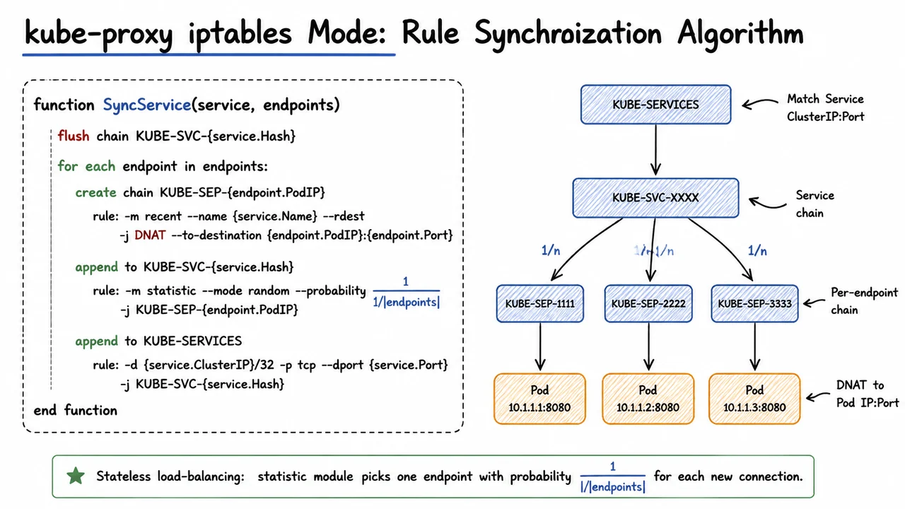
The core of the algorithm is a function, conventionally named SyncService, that takes a Service definition and its current list of healthy endpoints. The first action is destructive: it flushes the Service-specific chain, KUBE-SVC-{service.Hash}, removing all previously installed rules. This clean‑slate design sidesteps the complexity of incrementally adding and removing per‑endpoint rules in a concurrency‑safe way. However, it also means that during the flush‑and‑rebuild window, packets arriving for the Service may be dropped or processed against an incomplete rule set. The trade‑off has historically been considered acceptable because endpoint changes are relatively infrequent in stable clusters, and the iptables rule modifications themselves happen atomically at the netfilter level.
After flushing, the algorithm iterates over the set of surviving endpoints. For each endpoint, it creates a dedicated chain with a name like KUBE-SEP-{endpoint.PodIP}. This per‑endpoint chain contains the actual DNAT (Destination Network Address Translation) rule that rewrites the packet’s destination to the Pod IP and port. The rule uses the recent module to optionally enforce session affinity, but in the simplest case its job is pure translation:
This indirection—a separate chain per endpoint—keeps the main Service chain tidy and makes debugging much easier than inlining every DNAT rule directly.
The key load‑balancing logic sits inside the Service chain itself. For each endpoint, kube-proxy appends a rule to KUBE-SVC-{service.Hash} that uses the statistic module in random mode. The rule’s probability is set to , where the denominator is the current endpoint count. The exact iptables syntax skeleton is:
-A KUBE-SVC-{hash} -m statistic --mode random --probability P -j KUBE-SEP-{PodIP}
Because iptables evaluates rules sequentially, the first endpoint’s rule gets a probability of . If the packet does not match (i.e., the random draw fails), it falls through to the next rule, whose probability must be recalibrated to to maintain overall uniform distribution. kube-proxy performs this simple arithmetic as it iterates, effectively creating an on‑the‑fly cumulative distribution function that guarantees each endpoint receives an equal share of new connections. The algorithm terminates with an unconditional jump to the last endpoint if all previous stochastic rules miss—handling the case where rounding errors or integer arithmetic would otherwise let a packet slip through.
This probabilistic scheme yields a stateless load‑balancing decision: every new flow is routed independently, without any connection table maintained by kube-proxy itself. That independence is a strength, because it allows the data‑plane (the iptables machinery inside the kernel) to make per‑connection choices with near‑zero coordination overhead, but it also means that retries from the same client or correlated decision errors cannot be corrected by the proxy. Additionally, the quality of the uniform distribution relies on the kernel’s pseudo‑random number generator, which is fast but not cryptographically perfect—though in practice the bias is negligible.
Once the endpoint sub‑chains are wired together, SyncService finishes by inserting a top‑level dispatch rule into the KUBE-SERVICES chain. This rule matches packets destined for the Service’s ClusterIP and port, and jumps into the freshly assembled Service chain:
-A KUBE-SERVICES -d {ClusterIP}/32 -p tcp --dport {Port} -j KUBE-SVC-{hash}
All the components now form a tidy hierarchy: from KUBE-SERVICES to KUBE-SVC-*, through the probabilistic branching to KUBE-SEP-* chains, and finally to the concrete DNAT rules. The entire structure is regenerated per Service, per endpoint change, which keeps the rule‑building logic conceptually simple and enables swift introspection with standard tools like iptables-save.
The visual below consolidates this synchronization algorithm into a single glance. On the left, a clean pseudocode block captures the logical steps—flush, iterate, build per‑endpoint chains, and wire them with the statistic match. On the right, a miniature chain‑traversal diagram maps the concrete forwarding path: an arrow enters from KUBE-SERVICES, moves through the Service‑specific chain, and then fans out into three parallel endpoint chains, each labeled with the probability . From there, solid lines lead to Pod IP boxes, while the DNAT rule content is hinted inside the endpoint chains. This dual representation—code and topology—reveals how a declarative Kubernetes Service becomes an executable packet‑forwarding tree inside the Linux netfilter, rebuilt atomically the moment the set of healthy backends changes.
13. Ingress & Network Policies
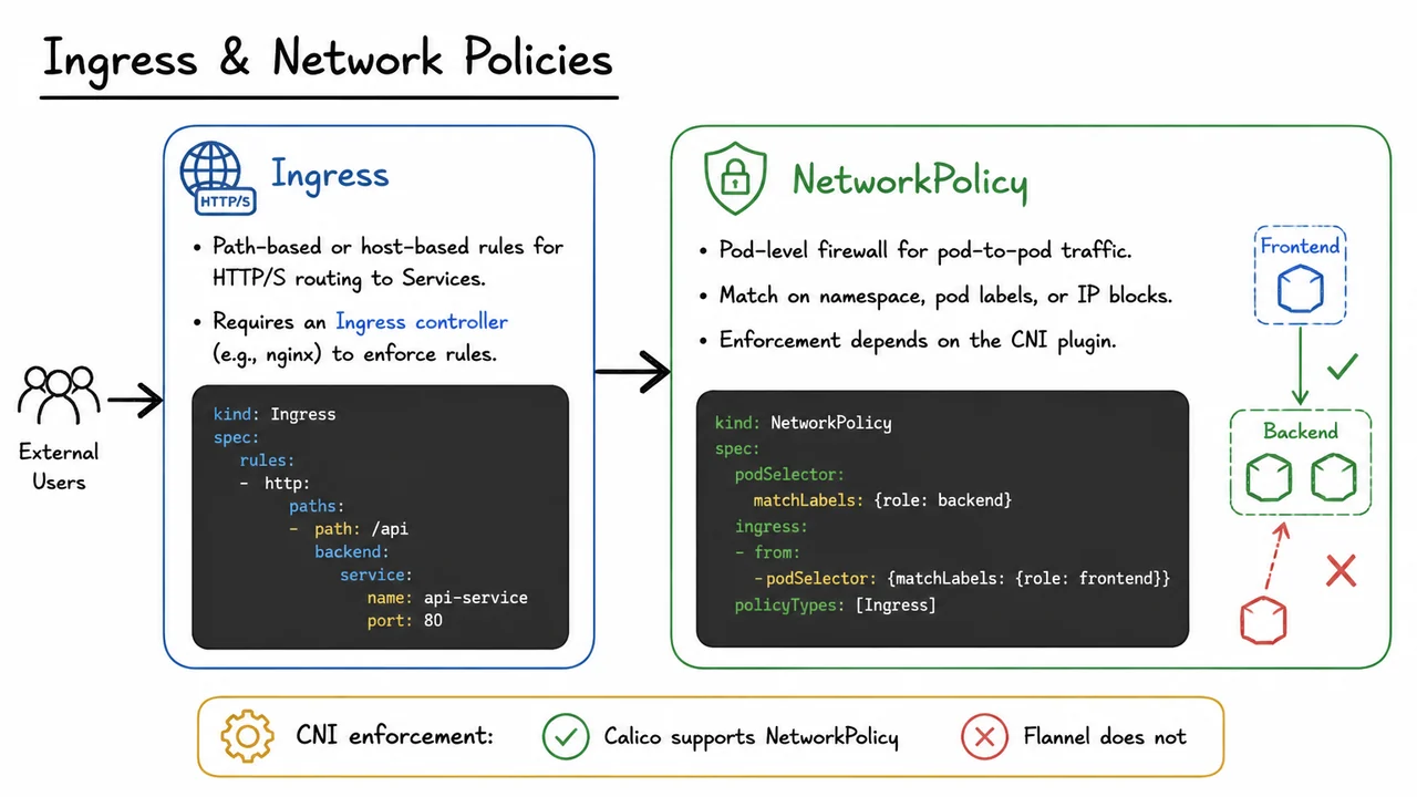
After we’ve established reliable internal service discovery and load‑balancing via ClusterIP and kube-proxy, we’re confronted with two new problems that any real‑world platform must solve: how do we steer outside HTTP traffic into the cluster, and how do we enforce fine‑grained security rules between workloads inside the cluster? Kubernetes answers these with two separate but complementary abstractions: Ingress for external HTTP/S routing and NetworkPolicy for pod‑level firewalling. They live at different layers of the networking stack, and their implementations reveal both the power and the responsibility placed on the cluster operator.
Ingress is best understood as an API object that captures intent, not a running piece of software. You write a manifest that declares, “for requests coming to my cluster, route those with host api.example.com and path prefix /api to the api-service Service on port 80.” The specification supports host‑based and path‑based rules, TLS termination annotations, and even fan‑out across multiple backends. But the Ingress resource on its own does absolutely nothing; it’s inert until you deploy an Ingress controller—a real workload (often an nginx, HAProxy, or envoy‑based pod) that watches the Kubernetes API for Ingress objects and translates their rules into concrete reverse‑proxy configuration. This division of labour is deliberate: the controller is the component that understands layer‑7 routing, handles TLS certificates, and often provides additional niceties like rate‑limiting or WAF capabilities, while the Ingress object offers a declarative, infrastructure‑agnostic interface. So a typical flow looks like this: external clients send HTTP requests to a load balancer (which may be cloud‑provided or an on‑premises solution) that forwards to the Ingress controller pods, which then parse the URL, look up the matching Ingress rule, and forward the request to the appropriate backend Service—ultimately landing on a pod inside the cluster.
From the perspective of the internal pod network, however, Ingress says nothing about who can talk to whom within the cluster. By default, Kubernetes imposes no restrictions: any pod can connect to any other pod or Service, across namespaces. That flat “all‑access” model is convenient during development but quickly becomes a security liability in production. Enter NetworkPolicy, a resource that acts as a label‑based firewall. Using a simple selector (podSelector) you pick a set of target pods, and then you define ingress rules that specify which sources are allowed to send traffic to them, and optionally egress rules that control where those pods may send traffic themselves. Sources can be matched by pod labels, namespace labels, or IP‑block CIDRs, giving you the flexibility to express micro‑segmentation policies like “only pods with label role: frontend may reach pods with label role: backend on port 5432.” The policy is additive: if multiple NetworkPolicy objects select the same pod, the union of allowed traffic is permitted.
There’s a critical caveat that often surprises newcomers: NetworkPolicy enforcement depends entirely on your CNI plugin. Kubernetes itself does not include a policy engine; it merely stores the NetworkPolicy resources in etcd and exposes them through the API. It is the container network interface plugin that must actually implement the filtering—typically by programming iptables, eBPF, or OVS rules on the host. Not all CNI plugins support NetworkPolicy. For instance, Calico provides first‑class policy support and even extends the standard NetworkPolicy with its own richer NetworkPolicy‑like resources; Flannel, on the other hand, historically does not implement any policy enforcement at all. This means that if you blindly apply a NetworkPolicy on a cluster using a non‑supporting CNI, it will silently have no effect—a dangerous situation that underscores just how tightly the networking stack is coupled to the plugin you choose.
The two abstractions—Ingress and NetworkPolicy—fit together in a layered defense. Ingress controls what arrives from the outside world (north‑south traffic) and gives you path‑based routing, SSL offloading, and external load‑balancing. NetworkPolicy governs east‑west traffic inside the cluster, reducing the blast radius of a compromised pod. Together they form a compelling security posture: only specific, well‑defined external requests reach your internal services, and once inside, those services observe the principle of least privilege.
The visual below distills this into a compact, side‑by‑side comparison. On the left, an Ingress box uses a highlighted YAML excerpt to illustrate a path rule forwarding /api to the api-service Service, while the accompanying bullet points remind you that an Ingress controller is required for this to take effect. On the right, a NetworkPolicy box shows a policy that uses podSelector to target backend pods and permits incoming traffic only from pods labelled role: frontend. A grey arrow flows from left to right, capturing the idea that external traffic passes through Ingress and then may be further restricted by NetworkPolicy. A callout at the bottom reinforces the hard‑learned lesson: “CNI enforcement: Calico supports NetworkPolicy; Flannel does not.” This diagram functions as a quick visual reference for the two objects that every administrator must master to make Kubernetes networking both accessible and safe.
14. Worked Example: E‑Commerce App on Kubernetes
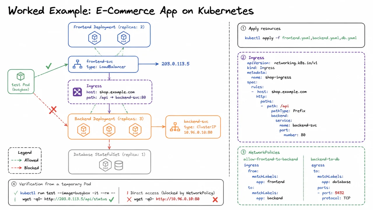
We have now walked through Ingress controllers that expose HTTP routes to the outside world, and NetworkPolicies that fence off internal microservices. The real test of understanding these primitives is to see them all working together in a realistic, multi‑tier application. This section assembles an e‑commerce stack—a frontend web store, a backend API, and a PostgreSQL database—and shows how Deployments, Services, Ingress, and NetworkPolicy combine to deliver a secure, externally reachable system. The orchestration is not a theoretical checklist; every resource plays a concrete role in scaling, discovery, traffic routing, and policy enforcement.
The application is split into three logical tiers. The frontend serves a JavaScript single‑page app to browsers, the backend exposes a RESTful API for product listings, cart, and checkout, and the database stores persistent order and inventory data. Because frontend and backend pods are stateless and benefit from sideways scaling, they are defined as Deployments with replica counts of two and three, respectively. The database, conversely, needs a stable network identity and persistent storage—even with a single replica—so it runs as a StatefulSet. The entire set of manifests is applied with one command:kubectl apply -f frontend.yaml,backend.yaml,db.yaml
With the workloads running, reachability is constructed through Services and an Ingress. The frontend Deployment gets a Service of type LoadBalancer, which provisions an external cloud load balancer that receives traffic at a public IP, here 203.0.113.5. The backend Service is of type ClusterIP with address 10.96.0.10:80—reachable only from within the cluster. An Ingress resource then bridges the two: it declares that any request arriving at host shop.example.com with path /api/… must be forwarded to backend-svc on port 80. An Ingress controller (commonly NGINX or a cloud‑native implementation) watches for this resource and reconfigures its routing table accordingly. Thus a user’s browser hitting http://shop.example.com/api/status will traverse the load balancer, be matched by the Ingress controller, and land at the backend API without exposing the backend Service address directly.
Up to this point, networking is wide open inside the cluster. Without NetworkPolicy, any pod could probe backend-svc:80 and talk to the database, violating the principle of least‑privilege. Two NetworkPolicy objects lock down the communication.
allow-frontend-to-backend: allows ingress traffic from any pod bearing the labelapp: frontendto any pod withapp: backendon port 80.backend-to-db: allows egress traffic from backend pods to the database pod on TCP port 5432.
These policies might be enforced on top of a default‑deny ingress/egress posture, so any traffic not explicitly permitted is dropped. The key insight is that the backend Service’s ClusterIP remains accessible to every pod by its IP, but the NetworkPolicy restricts which pods can actually send packets to the backing endpoints. The service is a stable name, not a security boundary; the policy creates the real enforcement.
To verify the setup, we spin up a temporary test pod—a minimal busybox container with no application label—and issue two HTTP requests.
wget -qO- http://203.0.113.5/api/status✅ — succeeds because the packet flows through the external load balancer, gets routed by the Ingress controller (which either runs with a matching label or is trusted via a broader ingress rule), and eventually reaches a backend pod.wget -qO- http://10.96.0.10:80❌ — fails because the test pod does not haveapp: frontend; the NetworkPolicy intercepts the connection attempt and drops it before it can reach the backend pod.
This demonstration encapsulates two essential lessons. First, an Ingress‑controlled path can remain externally available while internal direct access is blocked, giving a single application different trust levels for inbound traffic from outside vs. from arbitrary internal clients. Second, NetworkPolicy is the final arbiter of pod‑to‑pod communication; a service’s ClusterIP is no substitute for a deny rule.
The visual that follows this section brings every piece together in a clean, layered diagram. On the left, a tiered architecture shows the frontend Deployment with its two pods in blue, the backend
15. Summary: Kubernetes Architecture & Networking Stack
Having walked through a realistic e‑commerce deployment that traded a shell‑script nightmare for a few declarative YAML files, the natural question is: what exactly makes this possible? The answer is not a single magic bullet but a carefully layered architecture where each component plays a narrow, well‑defined role, and where the networking model is built from four distinct abstractions that together give us identity, reachability, load balancing, and security. The final slide of this lecture distills that whole picture into a compact visual—two summary tables that you can carry as a mental cheat sheet. But before we glance at the diagram, it is worth pulling the threads apart one more time so that the “why” behind each entry is clear.
At the top of the stack sits the API server, the single front‑end to which every other component—human users via kubectl, internal controllers, and even node agents—talks exclusively through REST calls. It is the declarative hub: you post a desired state (a Pod template, a Service, a NetworkPolicy), and the API server persists it into etcd, a strongly consistent distributed key‑value store. This store is the source of truth; losing etcd means losing the cluster’s memory. From that point on, the system diverges into two planes. The control plane houses the scheduler and the controller manager. The scheduler watches for Pods that have not yet been assigned a Node and places them by evaluating resource requests, affinities, taints, and tolerances. The controller manager runs a collection of reconciling loops—ReplicaSet, Endpoints, Node, and many more—each continuously comparing the recorded desired state against reality and issuing corrective commands back through the API server. Crucially, these components do not talk to one another directly; they all watch the API server, making the control plane loosely coupled and horizontally scalable.
On every worker Node, three critical agents convert those abstract objects into running processes. The kubelet is the Node’s sheriff: it receives Pod specifications and, via a container runtime (containerd, CRI‑O, or any OCI‑compliant engine), ensures the required containers are started, health‑checked, and terminated. The kube‑proxy maintains network proxying rules—written as iptables chains or as IPVS virtual servers—so that the virtual Service abstraction (a stable ClusterIP that never changes) always maps to one of the potentially ephemeral Pod IPs backing it. Finally, the CNI (Container Network Interface) plugin is the pluggable piece responsible for assigning each Pod a unique, routable IP address, wiring up an overlay or BGP‑based flat network, and enforcing any NetworkPolicy rules that restrict east‑west traffic. Together, these three turn a bare machine into a Kubernetes Node.
From a networking perspective, the stack can be read in four layers—each solving a different connectivity challenge. The foundation is the Pod network: a flat, non‑NATted address space in which every Pod can reach every other Pod (even across Nodes) directly by IP. This is not magic; it is an explicit design requirement that any conformant CNI plugin must fulfill, whether by VXLAN overlays, direct L3 routing with BGP (as Calico does), or host‑gateway schemes. Above that sits the Service network, a virtual address space where a stable ClusterIP fronts a dynamic set of Pod endpoints. kube‑proxy programs either a forest of iptables DNAT rules (randomly picking a backend) or an IPVS table (more efficient, with scheduling algorithms) to implement this load balancing. Notice that the Service network never physically exists: it is pure programming of each Node’s kernel.
External traffic enters through a third layer: NodePort opens a high port on every Node; LoadBalancer integrates with a cloud provider to allocate an external IP; and Ingress controllers provide layer‑7 HTTP routing, TLS termination, and path‑based forwarding—all defined declaratively. Finally, the NetworkSecurity layer uses NetworkPolicy objects to enforce zero‑trust micro‑segmentation. Unlike a traditional firewall rule that talks about IP addresses, a NetworkPolicy selects Pods and namespaces by labels and specifies allowed ingress/egress paths. Enforcement is the CNI plugin’s job (e.g., Calico translates policies into iptables or eBPF programs). Together, these four layers let you declare: “the checkout service should accept only TCP/8080 from frontend Pods in the web namespace,” and the network will enforce it without touching application code.
The summary visual that follows echoes this layered decomposition. It arranges the major architecture components into a two‑column table—one column naming the component, the other stating its unique purpose in a single sentence. This table immediately highlights the division of labour and reminds you that kube-proxy is not a single per‑cluster process but a per‑Node daemon. The second table maps the networking stack across four rows, linking each abstraction layer to its concrete implementation. The Pod network row emphasises the flat, IP‑per‑Pod guarantee; the Service row calls out iptables vs. IPVS; external access enumerates the three standard exposure methods; and the security row makes visible that NetworkPolicy enforcement depends entirely on the chosen CNI plugin. Together, the tables serve as a quick‑reference panorama of everything covered in the lecture—from the API‑server‑as‑hub model down to the last iptables rule. Keeping this mental model fresh will help you reason about failure modes (like a kube‑proxy crash leaving a Node unable to load‑balance) and design decisions (choosing a CNI that supports NetworkPolicy if zero‑trust is a requirement).