Large language models are astonishingly good at producing plausible text, yet the metric they were trained to optimize—next-token likelihood—is not the same as being helpful, honest, or safe. A pre‑trained model has absorbed statistical patterns from web‑scale data, including biases, toxicity, and factual errors. The central challenge of alignment is to steer these models so that their outputs reflect nuanced human values without sacrificing the fluency and generality we paid so much to acquire.
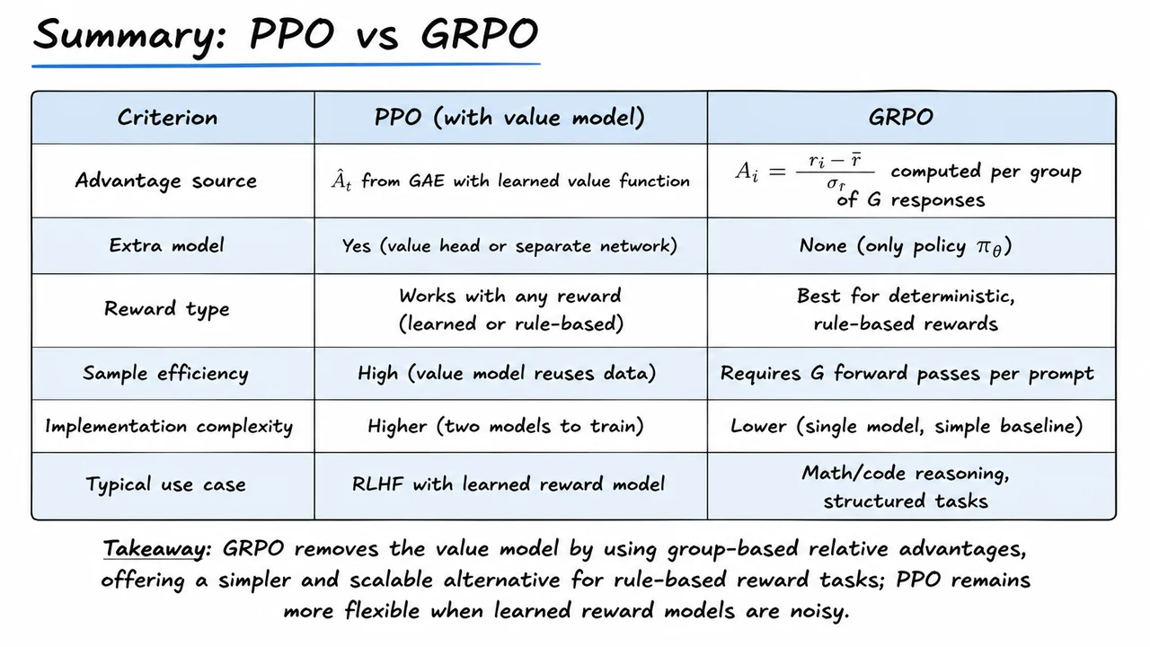
Supervised fine‑tuning (SFT) is a natural first step: we collect high‑quality demonstrations of desired behavior and train the model to imitate them. SFT teaches the model the stylistic conventions of a helpful assistant, but it cannot directly optimize for qualitative objectives that are inherently comparative or context‑dependent. A response that is truthful yet unhelpful, or safe but evasive, is hard to penalize with a fixed dataset of positive examples. SFT essentially copies the distribution of the demonstrations—it minimizes the forward KL divergence to the data. The model learns to reproduce the style of the examples, not to pursue abstract objectives like “be honest whenever possible” or “avoid harmful advice even when the prompt is ambiguous.” This gap between imitation and optimization is the reason reinforcement learning enters the picture.
Reinforcement learning from human feedback (RLHF) recasts alignment as a reward‑maximization problem. Instead of hand‑writing a reward function, we enlist human annotators to compare pairs of model outputs and express preferences. A separate reward model is trained to predict those human judgments, acting as a proxy for the true, hard‑to‑specify objective. Then we treat the language model as a policy that generates a response given a prompt , and we use RL to update to maximize the expected reward. Crucially, the update also includes a penalty that keeps the policy close to a frozen reference model (usually the SFT model), preventing the policy from drifting into nonsensical but spuriously high‑reward regions. The objective becomes something like:
where controls the strength of the KL regularizer. This framework can optimize for complex, human‑defined criteria that are not captured in any static dataset, and it enables the model to explore a range of responses while learning which ones are preferred.
The most widely used algorithm for RLHF is Proximal Policy Optimization (PPO). PPO alternates between sampling batches of responses, evaluating them with the reward model, and performing several gradient updates on the policy while clipping the update size for stability. A critical component is the value function, a learned critic that estimates the expected future reward from a given state (partial sequence). The value function is used to compute advantages, which reduce the variance of policy gradient estimates. However, maintaining a separate value model at the scale of modern LLMs introduces significant engineering and sample‑efficiency burdens: the value network must be roughly as large as the policy to be accurate, it needs its own training loop, and it can introduce estimation errors that destabilize training.
This bottleneck motivates a search for value‑free alternatives. Group Relative Policy Optimisation (GRPO) is a recent method that dispenses with the learned value function entirely. It works by sampling a group of responses for each prompt, scoring them all with the reward model, and then computing a relative advantage for each response by comparing its reward to the group mean and standard deviation. The policy is updated to favor responses that are better than average within their local group, while still constrained by a KL penalty relative to the reference policy. This replaces the global value‑baseline of PPO with a local, prompt‑specific baseline computed from the batch itself, dramatically simplifying the training pipeline and reducing the memory and compute footprint.
The lecture unfolds along a clear arc. We begin by revisiting the essentials of RL for text generation—policy gradient, PPO, and the role of the value function. Then we examine the standard PPO–RLHF pipeline in detail, highlighting its reliance on a separately trained value model. From there we diagnose the bottlenecks that appear when scaling value‑based methods to large models, which sets the stage for GRPO as a value‑free alternative. Finally, we compare the empirical performance of GRPO against PPO on mathematical reasoning benchmarks and discuss open questions around stability and reward hacking.
The visual below consolidates these ideas. On the left, two parallel pathways branch out from the pre‑trained language model: one labeled SFT (copy style, not objectives) and another labeled RLHF, which expands into a closed loop—policy sampling, reward evaluation, and an update that balances the reward signal against a KL penalty from the frozen reference model. On the right, a vertical outline charts the lecture’s progression from RL fundamentals through the value‑function bottleneck to the value‑free GRPO alternative, mirroring the conceptual journey we have just traced. This diagram gives you a mental map of where we are headed, and each component will be unpacked in depth as we move through the sections.
Despite the remarkable fluency and factual recall that large language models acquire during pretraining and supervised fine‑tuning (SFT), a critical vulnerability remains: the model has no intrinsic mechanism for verifying the correctness of the statements it produces. SFT trains the model to maximize the likelihood of token sequences in the training corpus, which encourages the imitation of surface-level patterns but not the underlying reasoning that guarantees truth. This gap becomes painfully clear when we examine tasks that require multi‑step logical deduction or strict adherence to mathematical rules. A model can eloquently reproduce a standard proof structure and still stumble at the final, crucial step—simply because its training objective never demanded that it distinguish between a correct conclusion and a subtly wrong one.
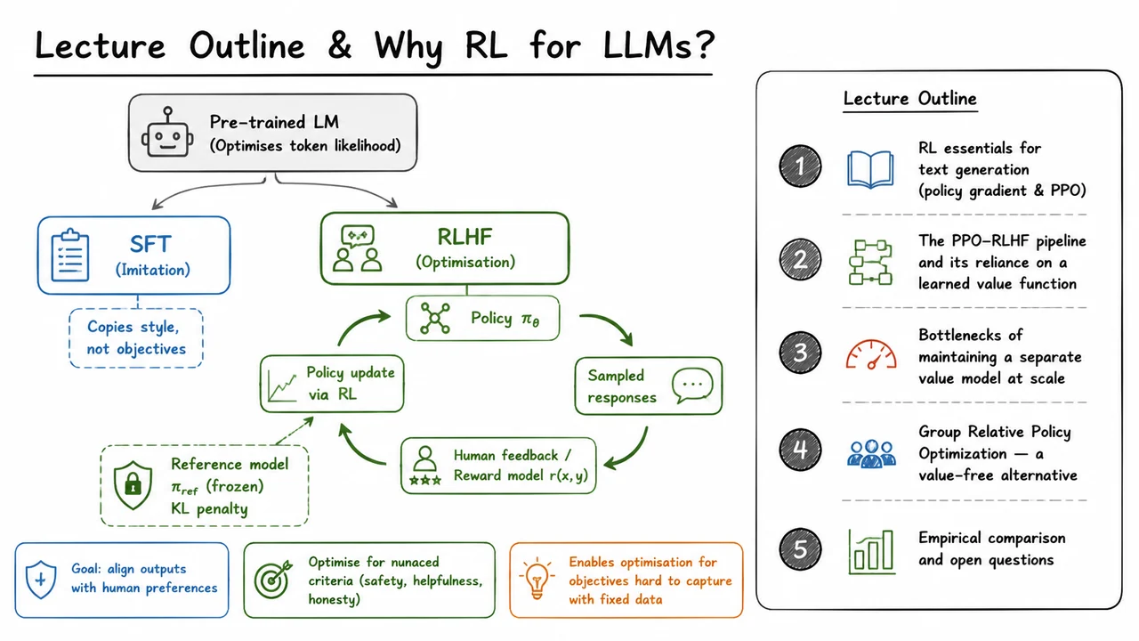
Consider the classic proof that is irrational. The argument proceeds by contradiction: assume with integers having no common factors. Squaring yields , implying is even, hence is even. Writing and substituting back gives , so is even as well. Both and are even, contradicting the assumption that they are coprime. The only logical conclusion is that such a representation cannot exist— is irrational. A supervised fine‑tuned model may output every line of this derivation flawlessly, only to cap it with “hence is rational.” That single erroneous word, when it appears, is not a typo but a symptom of a deeper mismatch: the model has learned to generate a plausible‑looking proof, not to bind the final statement to the preceding contradiction.
Why does SFT allow such a mistake? The training process optimizes the log‑likelihood of each token given its context, effectively asking: “Given the sequence so far, what token comes next in the training data?” In a large corpus of mathematical proofs, the word “irrational” may be much more common after this line of reasoning, but its antonym “rational” also occurs in other proof contexts. If the model’s distribution slightly favors the incorrect token, perhaps because of a co‑occurrence pattern in imperfect data or because the proof skeleton leads to a decision point with two plausible continuations, SFT has no external signal to penalize that choice. The loss function is blind to factual correctness; it only cares about predicting the observed text. Consequently, the model can become a vivid confabulator—a fluent generator of sequences that follow stylistic and syntactic norms but lack a truth‑grounding backbone.
This is not an isolated quirk of mathematical proofs. In any domain where correctness is governed by hard constraints—legal reasoning, code generation, scientific explanation—SFT alone risks producing outputs that are plausible yet false. The model may even insert circular arguments or omit subtle case distinctions because those patterns were rare in the training corpus. The example of the proof is especially pedagogical: the error flips the entire meaning with a single token, making it glaringly obvious, but similar logic‑breaking blunders can hide in longer passages and mislead users who trust the model’s authoritative tone. Without a reward function that explicitly evaluates the value of the output, the model remains an imitator, not a verifier.
Reinforcement learning enters the picture as a tool to align the model’s generation process with a predefined consequence: a reward that measures correctness, safety, or helpfulness. In the RL‑tuned version, the same chain of equations , , and the eventual contradiction are generated, but now the final token is scored. If the model says “rational,” it receives a low reward; if it says “irrational,” it gets a high reward. Over many rollouts and updates, the policy shifts probability mass away from plausible‑but‑false completions and toward verified true ones. Crucially, the reward does not require a human to label every possible output—rule‑based verifiers (as in mathematical reasoning benchmarks) or learned reward models can act as automated judges. This is the essential motivation for techniques like Group Relative Policy Optimization (GRPO), which we will detail later: they repurpose sparse, structured rewards to guide the model toward reasoning that is not merely fluent, but factually correct.
The visual below—a compact side‑by‑side comparison—crystallizes this contrast. At the top, a single prompt asks for a proof. Two columns then mirror the outcomes: the left, labeled “SFT (imitation),” displays the flawed proof with the erroneous concluding statement “hence is rational” struck through in red. The right, labeled “RL‑Tuned (reward optimized),” shows the identical derivation but ends with the correct statement “Therefore is irrational,” accompanied by a green checkmark. Below both boxes, a caption explains the core failure: SFT maximizes likelihood without verification, rewarding surface fluency over logical soundness, while RL with a correctness reward pushes the model toward verifiable truth. The image does not merely repeat the text; it gives you, at a glance, a visual anchor for the abstract limitation—a reminder that without a reward signal, a model can perfectly mimic the shape of a proof and still get the answer wrong. As we move into the mechanics of RL‑based alignment, keep this picture in mind: the only difference between the two columns is the training objective, and that single change transforms a convincing liar into a reliable reasoner.
Supervised fine‑tuning teaches a model to imitate a curated set of desirable outputs. That approach works well when the goal is to produce text that looks like high‑quality human writing—fluent paragraphs, correct formatting, safe‑seeming boilerplate. But alignment often demands more: a model should not merely mimic a distribution; it should solve multi‑step reasoning tasks, produce factually correct answers, or follow instructions that are easy for a human to check but fiendishly hard to cast as a local token‑level loss. These objectives are naturally expressed as a reward that can be evaluated over whole sequences, whereas cross‑entropy only ever sees one token at a time and cannot plan for long‑horizon consequences. When SFT is all we have, the model learns to pad its outputs with plausible‑looking filler but rarely learns to actually get the right answer under a verifiable criterion.
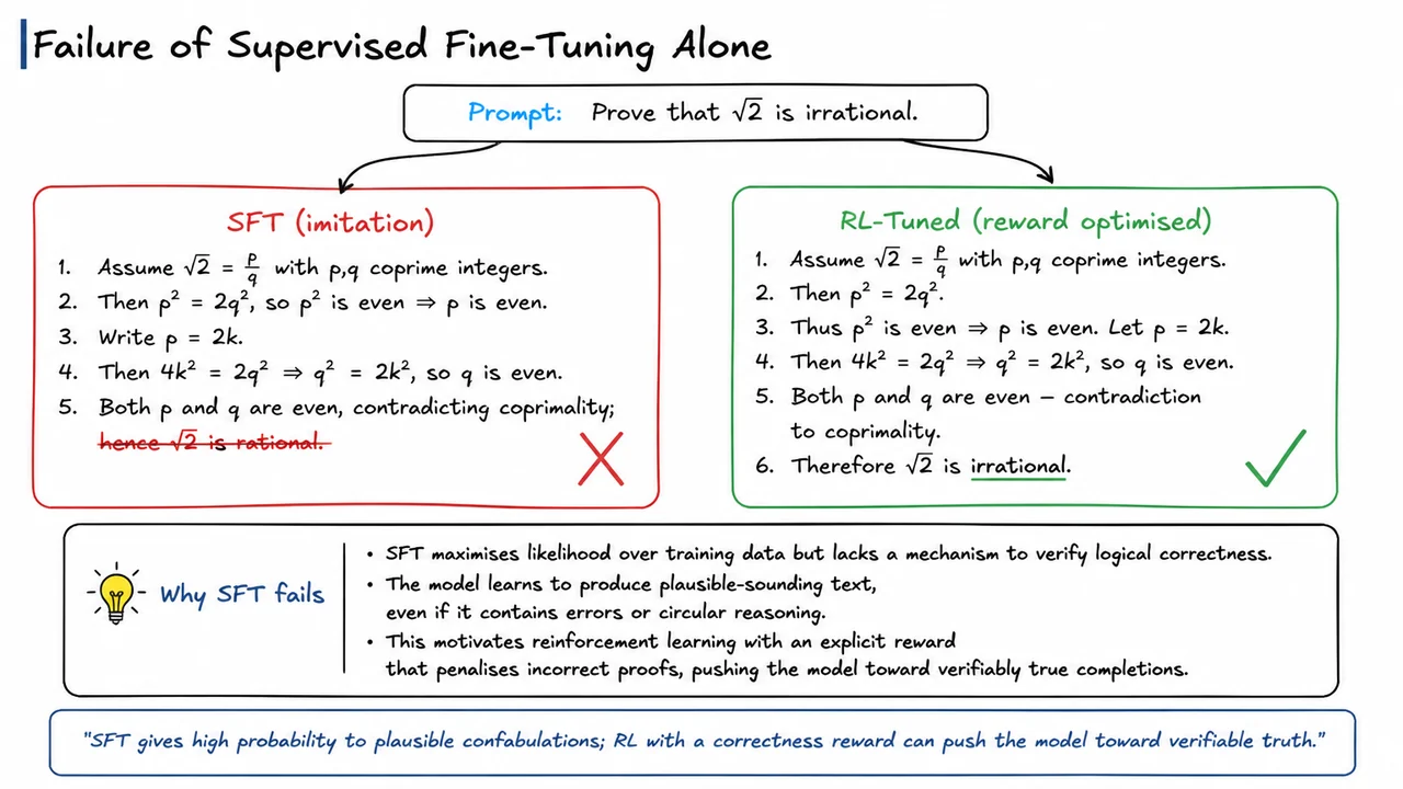
This gap is precisely why reinforcement learning (RL) has become the dominant paradigm for aligning large language models. In the RL view, text generation is a sequential decision process: at each step the policy (the language model) chooses a token given the prompt and the tokens produced so far, and after the final token a scalar reward is computed by an external verifier—a learned reward model, a rule‑based checker, or even a human evaluator. The objective is no longer to match a single target sequence; it is to maximize the expected reward of the model’s own generated completions while staying “close enough” to the behavior the model already had before fine‑tuning. Formally, with a dataset of prompts , a policy parameterized by , and a reference policy (often the pre‑trained or SFT model), the typical RL alignment objective is
The KL penalty prevents the policy from drifting too far into regions where the reward model is poorly calibrated or the language model loses its general capabilities—a kind of regularised exploration that makes RL alignment practically tractable.
Earlier implementations of this idea, most famously PPO for RLHF, wrapped the language model in an actor‑critic loop: a separate value network estimated the expected future reward at each token, and the advantage function guided the policy update. PPO delivered impressive improvements in instruction following and harmlessness, but it came with substantial engineering overhead: maintaining a critic of comparable size, handling stale value estimates, and tuning a handful of sensitive hyperparameters. The critic also introduced a subtle failure mode: if the value function learned the wrong credit assignment, the policy could easily exploit it, leading to reward hacking despite the KL penalty.
The Group Relative Policy Optimization (GRPO) algorithm, introduced by Shao et al. (2024), strips away the value function entirely. Instead, for each prompt, GRPO samples a group of responses from the current policy, scores them with a (deterministic, rule‑based) reward, and computes a relative advantage inside the group—essentially how much better or worse each response is compared to the group’s mean reward. The policy is then updated to increase the log‑probability of responses that scored above the group average and decrease the log‑probability of those that scored below. This value‑free, relative estimation scheme is strikingly simpler than PPO while preserving the essential benefit: the model learns directly from the reward signal without needing to train a separate critic. Despite its simplicity, GRPO has proven highly effective on reasoning tasks where a verifiable reward (e.g., whether the final answer matches ground truth) is available.
The shift from purely imitative SFT to reward‑driven RL can be understood through a clear conceptual contrast:
The visual accompanying this section crystallizes that contrast. On one side, it depicts the SFT pipeline: a fixed dataset of prompt‑completion pairs, a standard next‑token loss, and a model that passively absorbs patterns. On the other side, it sketches the RL alignment loop: prompts are fed to the current policy, multiple completions are sampled (the group), each receives a reward from an external evaluator, and the relative advantages are used to update the policy without a value network. The arrows make explicit what the equations imply—RL transforms language model training from a static imitation problem into a dynamic, feedback‑driven optimization where the model actively learns from the consequences of its own outputs. This is the core insight behind using reinforcement learning as an alignment tool, and the foundation on which GRPO builds a lighter, more stable variant.
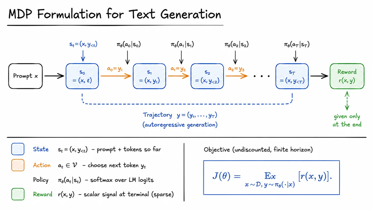
The last section established that reinforcement learning provides a principled framework for aligning language models with complex, human-defined objectives. But applying RL to text requires a precise mathematical abstraction that transforms token-by-token generation into a sequential decision problem. Fortunately, the autoregressive nature of language models lends itself naturally to a finite-horizon Markov decision process (MDP) with terminal reward. This formulation strips away many complexities of general RL while retaining exactly the structure needed to optimize sequence-level properties.
We start by defining the state at time step . The model has already produced a partial sequence conditioned on the prompt . The state therefore captures all the information that influences future generation:
Notice that the prompt is immutable and appears in every state; the only changing component is the growing prefix of tokens. This makes the state space enormous but structured, as each state is a concatenation of a fixed prompt and a variable-length token sequence.
The action is the choice of the next token from the vocabulary , which can be tens of thousands of tokens. This discrete action space is a defining feature of text-generation MDPs: high-dimensional, combinatorial, and heavily constrained by linguistic structure.
The policy is exactly the language model itself—a Transformer that maps state to a probability distribution over via logits, softmax, and a sampling strategy (e.g., greedy, temperature-scaled, or top-). The policy parameters encompass all model weights, and the whole generation process rolls out autoregressively:
A complete trajectory is the sampled sequence ; the sequence length may be variable, bounded by a maximum context length or terminated by a special end-of-sequence token. The horizon is finite by design—we never consider infinite text generation.
Crucially, the reward is not provided step by step. Instead, is a scalar signal delivered only at the end of the trajectory. This sparse, terminal reward model reflects real-world evaluation: we judge an answer, translation, or summary as a whole, not token by token. The reward might be a correctness checker, a learned preference model, or a rule-based function like “does the final answer match the ground truth?”. Because the reward arrives after the full sequence, credit must propagate back through all actions.
There is no discount factor in the objective. In infinite-horizon problems, discounting ensures convergence; here, the finite horizon eliminates the need for it. The objective simply maximizes the expected terminal reward over prompts and sampled trajectories:
This is the undiscounted expected return under the policy, with the expectation taken over the distribution of prompts and the model’s own generation stochasticity. Maximizing pushes the model to produce sequences that score highly according to the reward, effectively aligning the distribution with .
Why is this formulation useful? It makes explicit that text generation is a sequential decision process where each token choice shapes future possibilities and the final score. Standard supervised fine-tuning (next-token prediction) optimizes for token-level log-likelihood, which is myopic and prone to exposure bias; the MDP view instead exposes the entire trajectory to a global reward signal. Algorithms like policy gradient and GRPO can then directly estimate gradients with respect to , enabling fine-tuning that cares about the whole output—exactly what alignment requires.
A few important failure modes lurk behind this clean abstraction. The state space is astronomically large and partially observed in the sense that future rewards depend on the full sequence, making credit assignment challenging. The sparse reward can cause high variance in gradient estimates if not handled carefully. Moreover, the policy is already strong from pretraining, so naive exploration can quickly degrade performance; modern methods like GRPO introduce group-based baselines to stabilize training.
The visual below distills the MDP loop into a compact diagram. Starting from the prompt on the left, it tracks state transitions , each step governed by an action drawn from . The policy probability sits above the arrow, emphasizing that every token decision is stochastic and parameterized. After the final state , the trajectory terminates and yields the scalar reward , shown in green. The diagram intentionally omits a discount factor, reinforcing that this is a finite-horizon problem with terminal-only reward, and it uses color-coded blocks (blue for states, orange for actions, green for reward) to highlight the distinct components of the MDP. This is the complete formal scaffolding on which both classic RL algorithms and the modern GRPO method are built.
Having formalized text generation as a Markov decision process, we can now design a learning algorithm that directly increases the reward of the model’s sampled responses. The most direct approach is the policy gradient method, which estimates the gradient of the expected return with respect to the model parameters and then performs stochastic gradient ascent. This section reviews the foundational REINFORCE estimator and, crucially, the baseline trick that makes it usable in practice—ideas that later underpin both PPO and the value‑free GRPO algorithm.
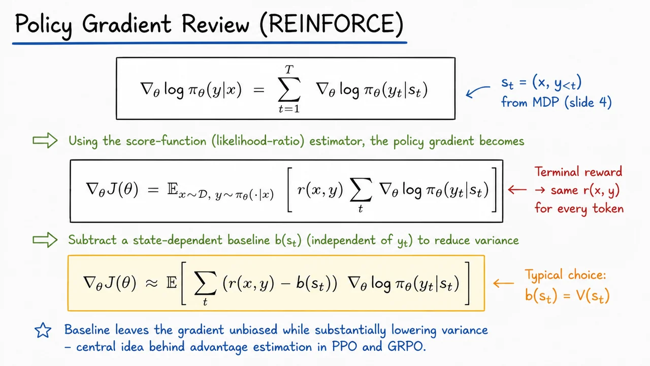
The log‑probability of a complete response given a prompt decomposes as a sum over timesteps because the model generates tokens autoregressively conditional on the state :
This linearity is essential: the gradient of the whole trajectory is simply the sum of per‑token gradients, each weighted by the same importance factor in the simplest estimator.
Applying the score‑function (likelihood‑ratio) trick, we can express the gradient of the expected return as an expectation over trajectories:
Because the reward is terminal and undiscounted, every token in the sequence receives the same scalar multiplier . This is an elegant property for language tasks where a meaningful reward only becomes available after the full response is generated, but it also introduces a major practical problem.
The raw REINFORCE estimator suffers from extremely high variance. Even with many sampled trajectories, the gradient signal is dominated by the magnitude of the reward (which can vary widely across prompts) and by the length of the sequence. Moreover, a uniformly positive reward would push all token probabilities in the same direction, while a uniformly negative one would suppress them, ignoring the fact that some tokens contribute more to the outcome than others. To make the estimator usable, we borrow a classic variance‑reduction technique: subtract a baseline that does not depend on the action . The modified estimator becomes
Since , the baseline leaves the gradient unbiased while offering a degree of freedom to shrink the variance. The ideal baseline would remove as much of the reward’s scale and noise as possible without introducing bias. A natural choice is the state‑value function , which represents the expected future return from state . An estimator of this value leads to the advantage , which measures how much better (or worse) the actual outcome is compared to what was expected at that timestep. This is the core insight that drives both PPO and GRPO.
The subtractive baseline directly anticipates the group‑relative trick that GRPO will later exploit. Instead of learning a separate value network—a costly auxiliary task that can introduce its own instability—GRPO constructs a baseline for each prompt by averaging the rewards of several independently sampled responses. That baseline is also unbiased (under mild assumptions) and dramatically reduces the variance, all while avoiding the need to model the environment’s value function. Understanding the classical baseline therefore bridges the simple REINFORCE estimator and the more sophisticated advantage‑based algorithms.
The visual below distills this derivation into a clean three‑equation progression. The top equation reminds us that the log‑probability of a response is just a sum of token‑level gradients. The middle equation presents the raw policy gradient, where every token shares the same terminal reward. The final equation, often highlighted to signal its practical importance, introduces the state‑dependent baseline and shows how subtracting it turns a crude scale‑dependent estimator into an advantage‑centered gradient update. This compact summary makes it easy to see why the baseline idea is not a minor tweak but the central mechanism for stable policy learning in language models.
The REINFORCE algorithm from the previous section offers an elegant, unbiased Monte Carlo estimator of the policy gradient. However, its simplicity hides a strict requirement: every trajectory used to compute the gradient must be drawn from the current policy . In practice, this on‑policy constraint is crippling. Modern deep reinforcement learning workflows typically collect a batch of rollouts, then perform multiple gradient updates on that same data to improve sample efficiency. The moment we reuse a rollout after even a single parameter update, the data becomes off‑policy—it was generated by an older policy , not the latest . Naively plugging those stale samples into the REINFORCE estimator yields a biased gradient and can rapidly destabilize training.
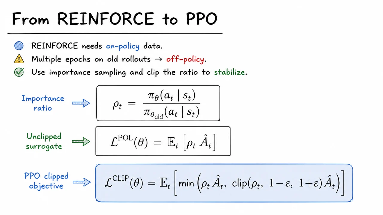
To fix this, we turn to importance sampling. For any trajectory fragment generated under , we can reweight the advantage by the likelihood ratio
This ratio exactly corrects for the distributional mismatch: multiplying the advantage by adjusts the contribution of each action so that, in expectation, the update points in the right direction. The resulting unclipped surrogate objective
recovers an unbiased estimate of the policy gradient when the expectation is taken under the old policy’s state‑action visitation. In theory, this lets us safely perform several epochs of updates on the same collected batch.
In practice, however, the unclipped surrogate can be treacherous. The importance ratio can drift far from 1 as the new policy diverges from the old one. A single large ratio combined with a positive advantage leads to an enormous, overconfident update that can permanently damage the policy. Conversely, tiny ratios with negative advantages may excessively suppress useful actions. The fundamental tension is between exploiting the data through multiple updates and constraining the policy change to a region where the importance sampling correction remains trustworthy.
Proximal Policy Optimization (PPO) resolves this by introducing a simple but highly effective clipped surrogate. Instead of trusting the raw ratio, PPO constrains the update to lie within a small interval , where is typically 0.1 or 0.2. The clipped objective reads
Here, the acts differently depending on the sign of the advantage. When (the action was better than expected), the objective increases as grows, but the clipped term imposes a ceiling at ; taking the minimum prevents us from accidentally raising the probability of a good action by more than a factor of relative to the old policy. Conversely, when , the objective decreases as gets small, but clipping at prevents us from driving the ratio below that floor. This asymmetric behavior makes PPO robust: it avoids the worst catastrophes of policy collapse without requiring a complex trust‑region optimization.
This single clipped surrogate became the standard policy loss in deep RL, including the PPO variant used in RLHF pipelines that fine‑tune large language models with human feedback. Its stability comes from the automatic reduction of the gradient when moves outside the safe region, effectively ignoring overly large steps that the importance sampling correction would otherwise encourage.
The visual below captures this progression from REINFORCE’s on‑policy limitation to the PPO clipped loss in a compact, equation‑oriented summary. The top equation defines the importance ratio , anchoring the off‑policy correction. The middle line shows the naive unclipped surrogate —the natural but dangerous extension. Finally, the bottom equation, highlighted in a distinct box, presents the full with its ‑and‑clip mechanism. Brief bullet points above remind the reader why off‑policy data arises and why clipping is necessary to prevent catastrophic updates. The layout encourages the student to see the three expressions as a logical ladder: importance sampling, the unstable objective it implies, and the clipped variant that makes PPO practical.
The transition from general policy gradient methods to their application in language model alignment is anything but straightforward. In previous sections we saw how PPO tames the high variance of REINFORCE by introducing a clipped surrogate objective and a learned value function baseline. When we move into the realm of large language models, the design of the reward signal and the baseline become deeply nontrivial because the environment is not a simulator but a human preference oracle—or, more pragmatically, a learned reward model. The standard RLHF pipeline, which we unpack here, layers three distinct training stages to turn a bare pretrained model into a policy that produces helpful, harmless, and preferred outputs. Understanding this pipeline—and especially the role of the separate value model it demands—is essential for appreciating why later innovations like GRPO dispense with that value model entirely.
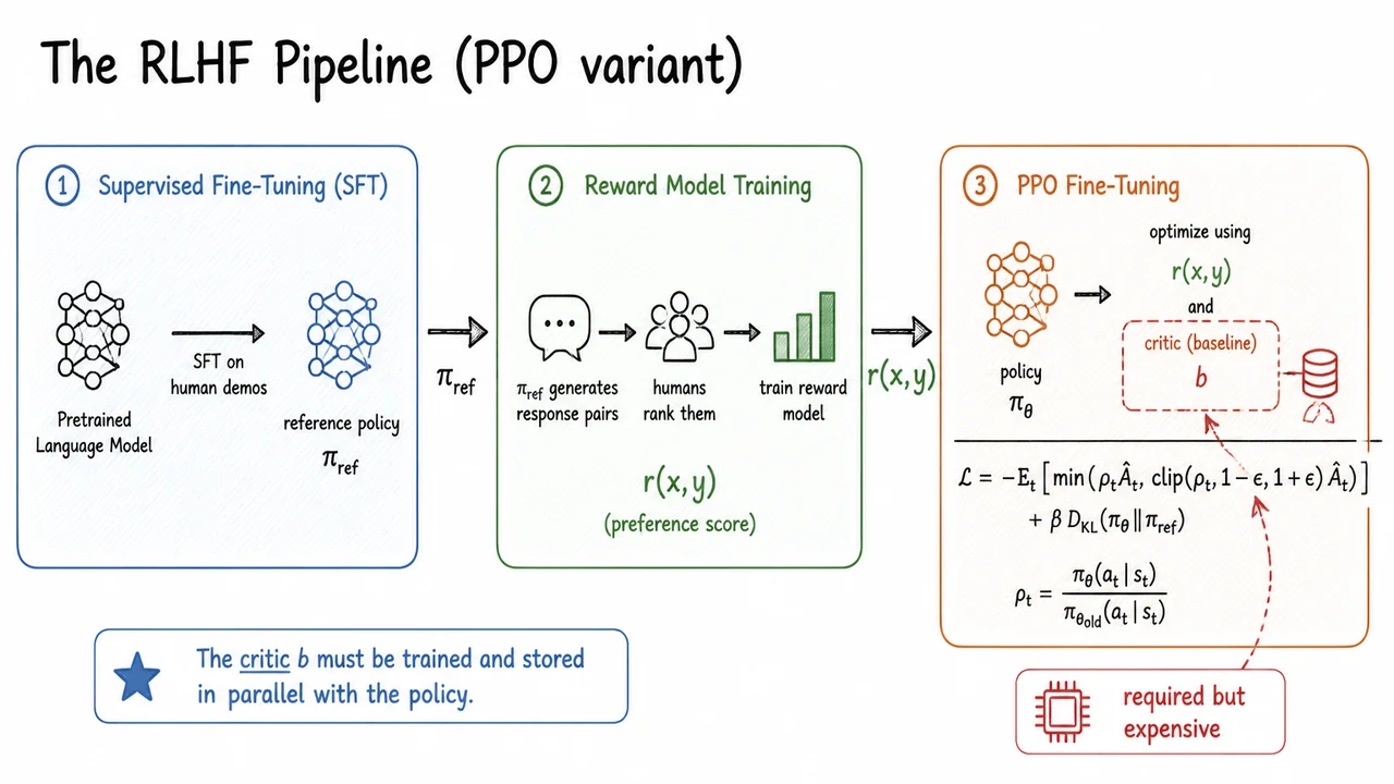
The first stage is Supervised Fine-Tuning (SFT). A pretrained language model is fine-tuned on a dataset of high-quality human demonstrations, typically prompt–response pairs collected from human annotators. This step already nudges the model toward fluent, relevant outputs, but it does not fully align it with nuanced preferences like helpfulness or safety because a likelihood-based loss cannot capture the relative quality between multiple plausible responses to the same prompt. The resulting SFT model is frozen and treated as the reference policy for the later RL stage. This reference is more than a checkpoint: it anchors the KL-divergence penalty that will prevent the policy from drifting into degenerate gibberish that happens to score highly on a narrow reward.
The second stage tackles the reward signal. Human annotators are shown multiple responses generated by for a given prompt and asked to rank them. These pairwise comparisons are used to train a reward model that predicts a scalar preference score for a prompt–response pair. Typically the reward model is initialized from the same SFT checkpoint and fine-tuned with a Bradley–Terry loss, learning to assign higher scores to responses preferred by humans. Crucially, this reward model now serves as the proxy for the true human preference function, and it will provide the reward in the subsequent RL stage. Yet it is a frozen, static function: it doesn’t itself adapt as the policy evolves, and it cannot be queried for expected future returns like a value function in a traditional MDP.
The third stage is PPO fine-tuning, where we finally treat response generation as a sequential decision process. The policy (initialized from the SFT model) now generates tokens autoregressively, and the reward model scores the finished sequence. To apply PPO we need an advantage estimate, and that requires a baseline. In classic PPO the baseline is the value function that estimates the expected future return from state . In RLHF we cannot simply roll out the environment; we need a separate value model —often called the critic—that regresses against the actual returns observed during training. This value model is typically a second, equally large language model head attached to the same backbone or a parallel network, and it must be trained alongside the policy using a mean squared error objective on the returns of sampled generations.
The PPO objective used in RLHF then becomes a composite loss. For each token-level step we compute the probability ratio between the current policy and the policy from the previous epoch. Using the advantage estimate from the critic, we form the clipped surrogate:
To keep the updated policy from diverging too far from the human-aligned SFT behavior, a Kullback–Leibler (KL) penalty weighted by is added, comparing the learned policy to the frozen reference :
This KL term acts as a regularizer, discouraging the policy from exploiting quirks of the static reward model and preserving the desirable generation patterns instilled during SFT.
The presence of the separate critic is at the heart of the complexity that GRPO later attacks. Training a value model in parallel with the policy doubles the memory footprint—both networks must be stored in GPU memory, and for modern 7B–70B parameter models that can be prohibitive. Moreover, the critic must regress against returns that are themselves noisy because they come from a single sampled trajectory evaluated by a frozen reward model; this regression often becomes unstable or learns slowly, introducing yet another source of variance into the policy gradient. The visual below consolidates the entire three-stage pipeline with a particular emphasis on this critic. You’ll see the flow from pretrained model to SFT and reference policy, to reward model training via human rankings, and finally to PPO fine-tuning where the policy and a dashed‑bordered critic box coexist inside the third stage. A red accent explicitly calls out the memory and compute overhead of maintaining that separate value network—overhead that the next section quantifies and that GRPO is designed to eliminate.
In the standard PPO‑based RLHF pipeline described earlier, the advantage of an action is computed as
where is the episode‑level reward and is a baseline supplied by a separately trained value model . While the subtraction of a baseline can reduce variance in principle, tying that baseline to a learned value function creates a nexus of practical difficulties that are especially acute when aligning large language models. Understanding these difficulties is essential, because they directly motivate the value‑free alternative that we will explore in the next section.
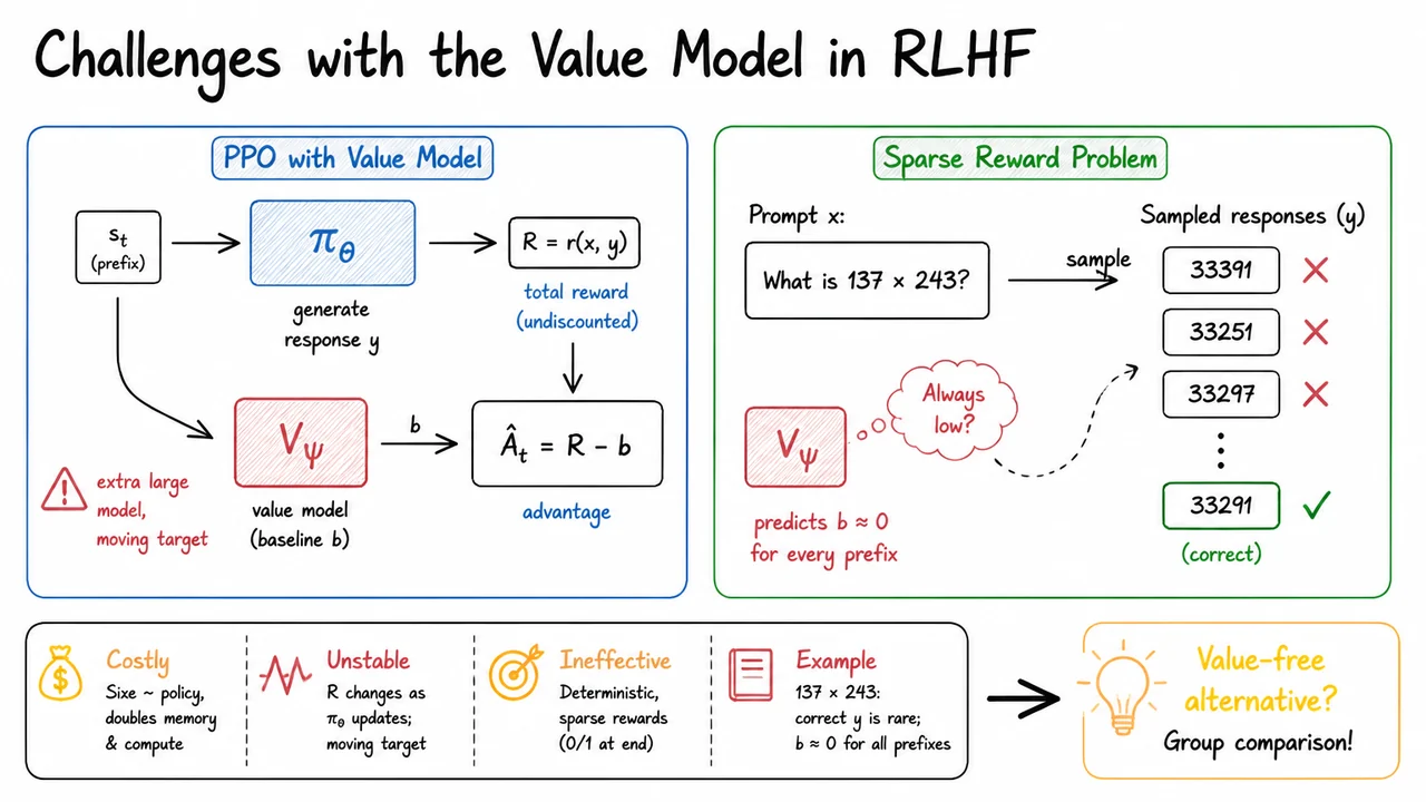
The most immediate burden is cost. A value model for an LLM must be comparable in capacity to the policy itself; otherwise it cannot internalise the linguistic and semantic context needed to judge a partial response. In practice, is often another large transformer of similar size—for instance, a second 7B‑parameter model sitting beside the policy—effectively doubling the memory footprint and per‑step computation. When GPU memory is already tight and every billion parameters matters, this extra model turns into a prohibitive tax, slowing experimentation and preventing the use of larger policy architectures.
Even if one can afford the memory, the value model introduces a fundamental instability. The target it tries to approximate—the expected future reward of an intermediate state—changes as the policy improves. In RLHF, the reward function may be fixed (e.g., a pre‑trained reward model or a rule‑based scorer), but the distribution of completions shifts with every gradient step. This turns into a moving target. Without careful tuning of replay buffers, trust‑region constraints, and learning rate schedules, the value model often diverges or oscillates, destroying the very variance reduction it was meant to provide. The stabilisation effort can easily dominate the project, shifting focus away from policy improvement.
A deeper flaw emerges when we examine the type of reward signals common in alignment tasks: many are deterministic and sparse. Consider a mathematical reasoning problem like . The reward is if the final answer is correct and otherwise, delivered only at the very last token. The outcome is deterministic: given a prefix, eventual correctness depends entirely on whether the remaining generation leads to the right result. In principle, a perfect value function could predict the probability of success from any prefix and thus provide a useful baseline. In practice, correct reasoning chains are rare, and the value model quickly learns a degenerate solution: for almost every prefix, the predicted baseline collapses toward . The few promising paths are not numerous enough to be distinguished from the many failures. As a result, the advantage becomes essentially the raw reward , and the PPO update loses all ability to perform fine‑grained credit assignment across tokens. The baseline once again adds no variance reduction.
This collapse is not a pathological edge case—it is symptomatic of any alignment domain with binary, end‑of‑episode rewards, such as code correctness checks, safety‑rule violations, or factual accuracy evaluations. In
Having established that training a value function in the standard RLHF pipeline brings significant computational cost and instability—especially when rewards are sparse, deterministic, and rule-based—we now turn to an elegant alternative that removes the critic altogether. The core question is: if the reward landscape is so simple that a learned baseline provides little variance reduction, can we design an advantage that is both cheap and stable without relying on a value head? The answer is Group Relative Policy Optimization (GRPO), which replaces the value network with a purely data‑dependent baseline computed from a group of responses sampled for the very same prompt.
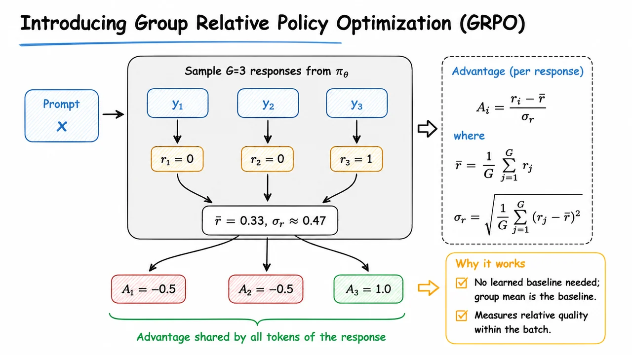
The central idea is disarmingly simple. For each prompt , instead of generating a single response and then having a critic estimate the expected return, we sample a group of independent responses from the current policy . Because these are all drawn from the same prompt and the same policy, the distribution of their rewards reflects the policy’s current competence and the difficulty of the prompt. We then compute the scalar reward for each response directly via the rule‑based verifier (e.g., checking whether the final answer matches a ground‑truth number). With these reward values, we define a per‑response advantage that is simply the z‑score of the rewards within the group:
where
This advantage is shared across all tokens of response . In subsequent policy gradient updates (whose full objective will be derived in the next section), it multiplies the log‑probability of each token in that response, steering the policy toward actions that increase the probability of high‑reward sequences and decrease the probability of low‑reward ones. Notice that no value function appears anywhere: the group mean plays the role of a local baseline, and the division by keeps the advantage scale from inflating when reward variance happens to be tiny.
To see how this works in practice, consider a typical binary reward setting where . With a group size , suppose we sampled three responses for a prompt and found the rewards . Then the group mean is and the standard deviation is . The resulting advantages are and . The correct response receives a strong positive signal, while the two incorrect ones receive a mildly negative signal. This relative scaling is what drives learning: the policy is encouraged to produce outputs that look more like the successful response and pushed away from patterns that lead to failures—all without ever needing to approximate a complex value landscape.
There are several important consequences of this design. No learned baseline means we avoid the memory footprint, training instability, and hyper‑parameter sensitivity associated with the critic. The advantage is purely relative inside the batch, so it automatically adapts to the difficulty of each prompt: harder prompts might yield many zeros and only a few ones, but the z‑score still correctly identifies the best and worst attempts. Furthermore, because the rewards come from a deterministic rule, there is no reward noise to confuse the baseline; the only stochasticity comes from the policy sampling, and the group‑based z‑score provides a consistent, low‑variance signal as long as is chosen appropriately. This makes GRPO especially well‑suited for mathematical reasoning and exact‑match tasks, where a large language model must learn to produce a precise final answer.
The trade‑off, of course, is that the advantage estimate’s quality depends on the group size . With very small the z‑score is noisy and the baseline can be poor; with very large the computational cost grows linearly. However, in practice, moderate group sizes (e.g., to ) have proved sufficient to deliver stable and effective fine‑tuning, as we will see in later empirical results.
The visual below distills this entire flow into a compact diagram. It begins with a single prompt in the leftmost box, from which the policy samples three independent responses . Each response is sent to the rule‑based reward function, yielding . These three numbers are funneled into a central computation block that calculates and , and then produces the z‑score advantages: a negative value () below the two incorrect responses and a distinct positive value () below the correct one. The grouping and the absence of any value network are made explicit by the surrounding box that marks the within‑batch comparison. The diagram thus serves as a one‑image summary of how GRPO eliminates the critic while preserving a strong learning signal through batch‑relative normalization.
Earlier, we saw how Group Relative Policy Optimization (GRPO) dispenses with the learned value function that standard PPO–RLHF requires, replacing it by a group-normalized reward signal computed entirely from rule-based feedback on multiple sampled responses per prompt. That shift eliminates the need to train and maintain a critic, dramatically simplifying the RL alignment pipeline. The next logical step is to transplant this new, value‑free advantage into the policy loss that will actually update the language model’s parameters. The derivation shows both the elegance of the substitution and the careful engineering needed to keep training stable without an explicit state‑value baseline.
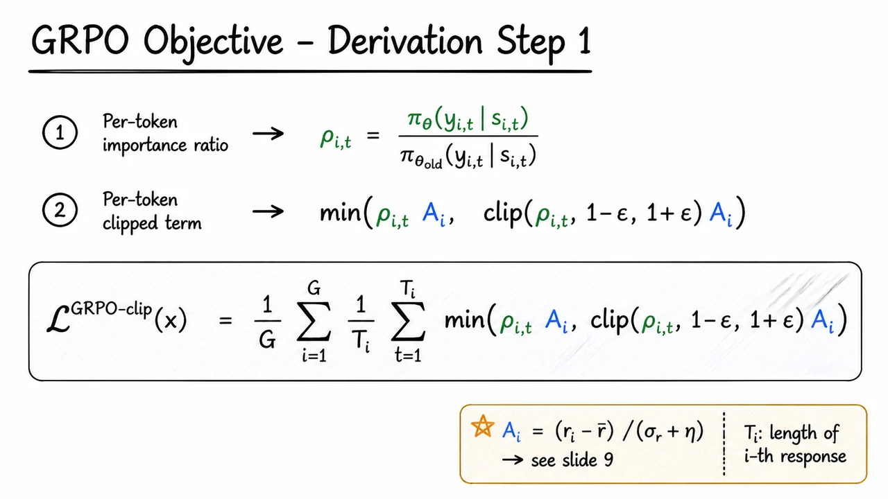
The starting point is the familiar PPO clipped surrogate. In a token‑level formulation, PPO computes a probability ratio between the current policy and the old policy that was used to generate response :
This ratio measures how much more or less likely the new policy considers token of response , given the preceding context . The genius of PPO’s clipping is that it trusts small ratio changes as reliable gradient signals, but heavily penalises large, destabilising updates by clamping the ratio to a narrow interval . In the original formulation, the ratio is multiplied by the token‑level advantage , which depends on a critic’s value estimate. Here we instead feed in the sequence‑level group‑normalised reward – a single number per response, constant for every token of that response.
Because is flat across the entire decoded sequence, the per‑token objective collapses elegantly. For a single token the clipped loss term becomes
The min operator acts as a pessimistic bound: it selects the smaller of the unclipped ratio‑advantage product and the clipped version. This prevents the policy from moving too far in “good” directions when is positive, yet still allows strong steps away from poor behaviour when is negative – a directional asymmetry that is critical for avoiding catastrophic forgetting and reward hacking. Crucially, the clipping is applied to only; the advantage itself is not clipped, which preserves the relative ranking among the group’s responses.
With the token‑level surrogate in hand, we still need a scalar loss for the entire prompt . GRPO follows a hierarchical aggregation: first average over the tokens of response , then average over the responses in the group for that prompt. This yields the per‑prompt GRPO clipped objective:
The double averaging ensures that each response contributes equally regardless of its length – shorter sequences are not artificially down‑weighted – and that the overall gradient is scaled by the group size . In practice this formulation works as a “local” policy gradient: the model is encouraged to increase the probability of responses that scored above the group mean, and suppress those below, but only to the extent that the probability ratio remains trustable (i.e., within the clipping threshold).
Two subtle consequences deserve emphasis. First, because is computed solely from rule‑based rewards after sampling all responses, there is no need for an external reward model or a value network; the entire RL signal is self‑contained within the prompt’s mini‑batch. Second, the use of underscores that the advantage is anchored to the behaviour policy that actually generated the responses, avoiding the off‑policy distribution shift that can destabilise online RL. As we shall see in the next section, a KL divergence penalty is later added to the final loss to further regularise the policy update, but the core of GRPO’s learning is already captured by this clipped objective.
The accompanying diagram condenses this derivation into a single visual argument. At the top, two small equation blocks recall the definition of and the token‑level clipped term, using green and blue accents to highlight the ratio and the advantage respectively. The centre of the slide is dominated by the large, carefully boxed expression for , with the nested summations made explicit. A callout in the bottom right corner points back to the group‑normalised advantage from the previous section, anchoring the viewer in the larger narrative. The clean, hand‑drawn aesthetic emphasises the logical flow: replace the critic with a group‑relative signal, keep the clipping, average over tokens and responses, and you obtain a stable, value‑free policy loss for LLM alignment.
Having derived the clipped surrogate term that encourages the policy to favour responses scoring above the group average, we now face a classic tension in RL fine‑tuning: as we maximise the reward‑weighted objective, the current policy can drift far from its initial behaviour. This is particularly dangerous for large language models because the reward signal – especially when rule‑based – is a noisy proxy for true quality. If left unconstrained, the model may exploit reward hacks (e.g., producing grammatically correct but logically empty outputs that happen to match a pattern the rule scorer rewards) while abandoning the fluent, diverse language it learned during pretraining and supervised fine‑tuning. Consequently, we need a regulariser that gently anchors the policy to a stable reference point.
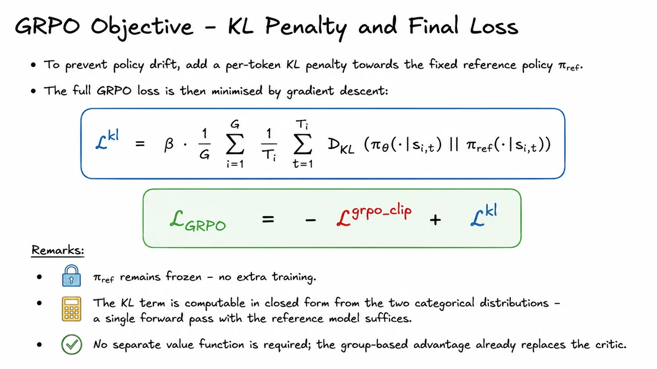
In Proximal Policy Optimization (PPO) as used in RLHF, a KL‑divergence penalty is added to the reward to keep the policy close to the supervised‑finetuned model. GRPO adopts the same idea but applies it in a value‑free setting. The reference policy is the pretrained and instruction‑tuned model frozen at the start of RL fine‑tuning. It never gets updated; we only query it to compute the KL divergence between its next‑token distribution and that of the current policy . The resulting KL penalty is defined as:
Let’s unpack the terms. is the number of responses sampled for the prompt (the group size), and is the token length of the -th response. For every token position in every generated sequence, we compute the KL divergence between the two categorical distributions over the vocabulary – ’s output probabilities and ’s output probabilities. Summing over all positions and responses gives the total divergence, normalised by and the respective sequence lengths so that each token contributes equally regardless of group composition. The hyperparameter controls the strength of the regularisation: small lets the policy move aggressively to maximise reward, while larger forces it to stay closer to the safe reference.
A crucial practical advantage is that this KL term is computable in closed form from the two probability vectors at each token – it is simply , which is a cheap operation compared to running a critic network. Moreover, we only need a single forward pass with the frozen reference model per batch of generated sequences; that pass can be done in parallel with other computations, adding minimal overhead.
The full GRPO loss is then assembled by combining the clipped policy‑ratio objective from the previous step and the KL penalty. Since we want to maximise the reward‑weighted objective, we minimise the negative of plus the regulariser:
This single scalar is all we need to back‑propagate through the policy parameters . Remarkably, no separate value function, no critic network, and no GAE (Generalized Advantage Estimation) are required. The group‑based advantage computed from the relative rewards already replaces the typical critic, and the KL penalty takes on the role of a soft trust‑region constraint. Because is frozen, the optimisation is stable – the regulariser does not introduce a moving target.
The visual below encapsulates this final objective structure. It displays the KL penalty equation in a prominent block, emphasising its per‑token, per‑group averaging character, and then shows the complete loss boxed beneath it as the sum that drives gradient descent. By glancing at the diagram, you can immediately see the two principal components: the clipped surrogate (represented conceptually by its negative) and the KL distance scaled by . Small callouts reinforce the three key practical remarks: the reference model is frozen, the KL divergence is closed‑form and cheap, and there is no critic in the loop. This visual consolidation helps the mind move from the algebraic derivation to a compact, intuitive formula you can recall when implementing or debugging GRPO.
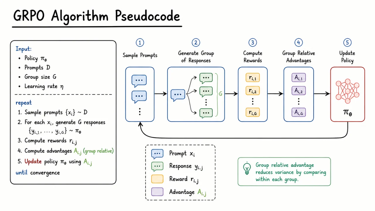
Having formalized the GRPO loss with its clipped surrogate and optional KL penalty, the natural next step is to ask: how do we actually run this optimization loop in practice? PPO famously requires an additional learned value function (the critic) to estimate advantages, which doubles the model size and introduces its own training instability, especially in the high-dimensional token-generation setting. GRPO sidesteps this entirely by replacing the value network with a simple, powerful idea—relative normalization across groups of responses sampled for the same prompt. The algorithm that emerges is streamlined, easy to implement, and retains the stable monotonic improvements PPO is known for, but without the critic’s baggage.
The GRPO algorithm operates in a classic on‑policy fashion, iteratively collecting experience and updating the policy. For each update step, we sample a batch of prompts from the dataset. For every prompt in the batch, we generate complete responses using the current policy . This yields response–reward pairs per prompt, where the reward for each response comes from a deterministic, rule‑based verifier (e.g., exact‑match accuracy, format compliance, or execution‑based unit tests). Crucially, these rewards are cheap to compute and need no human labelling, so large per‑prompt groups—often or higher—are feasible. The group constitutes the key statistical unit: all subsequent advantage calculations happen independently within each prompt’s group, not across the entire batch.
Once we have the group rewards, the algorithm computes group‑relative advantages. For a given prompt, let the rewards be . We compute the group mean and the group standard deviation . The relative advantage for the -th response is then:
with a small for numerical stability. This normalization acts as a robust, zero‑parameter baseline: responses better than the group get positive advantages, worse ones get negative advantages, and the scaling by standard deviation keeps gradients well‑behaved across prompts of varying difficulty. Because the group is generated with the same prompt, the relative comparison is meaningful—the prompt’s inherent difficulty is automatically cancelled out—and no value head needs to be trained to approximate expected future return.
With the advantages in hand, we can finally form the policy loss exactly as derived in the previous section: the clipped surrogate objective using these per‑token importance weights, plus the optional KL penalty term to keep the policy close to a reference model. The algorithm then performs a small number of gradient steps (often one full batch update) to maximise that objective, and then discards all sampled data—the whole process is strictly on‑policy. The loop repeats, each time sampling fresh responses with the latest policy parameters.
Compared to PPO–RLHF, GRPO trades a critic’s sample efficiency (since a value function can learn from old data) for algorithmic simplicity and stability. The per‑prompt group sampling may reuse many tokens for the same input, but because rewards are rule‑based, the additional cost is negligible relative to the LLM forward passes. In the domains where GRPO shines—mathematical reasoning, code generation, and other verifiable tasks—this trade‑off is overwhelmingly advantageous.
The visual summary that follows distills this algorithmic flow into a clean, Excalidraw‑style diagram. At the top you’ll see a prompt batch, which fans out into an iconic group of sampled responses. Each response gets a reward tag, and a central “Group‑relative norm” stage computes the standardised advantages inside a dashed box, highlighting the core insight. Arrows then converge into the policy update step, with a small callout reminding us of the clipped surrogate and optional KL penalty. The diagram is not a line‑by‑line replication of pseudocode, but a compact engineering sketch—exactly what you would want on a whiteboard to explain GRPO to a colleague. It reinforces the two-phase mental model: sample groups, normalise within them, then optimise, all without a critic in sight.
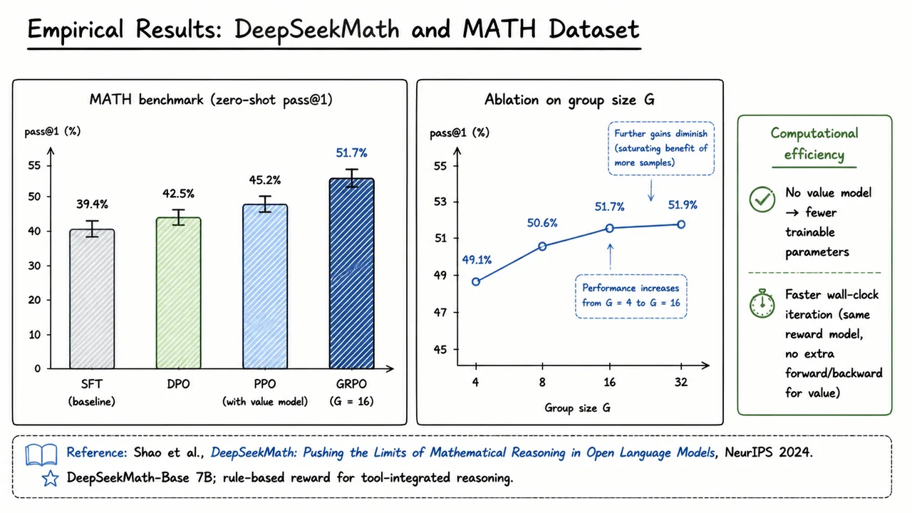
After stepping through the GRPO pseudocode, it is fair to ask whether this value‑free design actually delivers competitive alignment in practice. The answer comes from Shao et al. (2024), who applied GRPO to fine‑tune a 7‑billion‑parameter base model—DeepSeekMath‑Base 7B—on the challenging MATH benchmark. MATH is a collection of high‑school mathematics competition problems, and zero‑shot pass@1 accuracy on this dataset has become a standard measure of an LLM’s genuine mathematical reasoning ability. The fine‑tuning setup used a rule‑based reward that simply checks whether the final answer produced by the model’s chain‑of‑thought (which may include Python code executed in a sandbox for “tool‑integrated reasoning”) matches the ground‑truth answer. This deterministic, per‑response reward signal avoids the need for a learned reward model and makes the evaluation of RL algorithms particularly clean: improvements come entirely from better policy shaping under the same reward.
The head‑to‑head comparison on zero‑shot pass@1 tells a clear story. A pure supervised fine‑tuning (SFT) baseline on the MATH training set reaches 39.4%. Direct Preference Optimization (DPO) manages 42.5%, while standard PPO with a learned value model (using the same rule‑based reward) achieves 45.2%. GRPO with a group size of attains 51.7%—a jump of more than six percentage points over PPO and over twelve points above SFT. That GRPO not only matches but substantially surpasses PPO while eliminating the value model is remarkable. It suggests that the per‑group relative advantage computation is a more reliable signal for policy updates than a separately trained value function, at least in settings where the reward is deterministic and per‑sample rewards can be contrasted directly.
The computational savings amplify the appeal. Because GRPO discards the value head, the number of trainable parameters shrinks by roughly half compared to a typical PPO setup with a critic of comparable size. More importantly, wall‑clock iteration time drops because there is no additional forward/backward pass for the value model, no need to store value‑target buffers, and no reward‑model‑rollout orchestration beyond the existing on‑policy sampling. The same rule‑based reward function is used; the only extra cost is generating responses per prompt instead of a single rollout per PPO update. Yet, as the ablation on group size reveals, this cost is well‑modulated.
The second key empirical result is an ablation on group size . When is increased from 4 to 16, MATH pass@1 climbs steadily—from roughly 49% at to the peak 51.7% at . Beyond the curve flattens; the benefit of additional on‑policy samples saturates. This pattern is consistent with the idea that a handful of sampled responses are enough to form a reliable relative advantage estimate. Further samples add little new information about the typical reward distribution for a prompt, so policy updates stop improving. Saturation at a moderate also implies that GRPO can operate efficiently without needing the huge batch sizes that pure rejection‑sampling methods sometimes demand. In practice, or is often sufficient, keeping the sampling overhead manageable.
These results together validate the core hypothesis behind GRPO: for deterministic, rule‑based rewards, a value‑free policy gradient that uses per‑prompt groups of sampled responses to estimate advantages can provide stronger and more stable learning signals than PPO with a learned value function, all while being faster and simpler.
The accompanying figure consolidates these findings into a single, clear visual argument. The left panel is a bar chart with methods—SFT, DPO, PPO, GRPO ()—on the x‑axis and pass@1 accuracy on the y‑axis, where the tall dark‑blue bar for GRPO immediately dominates. The right panel shows a line plot of group size against pass@1; the curve rises steeply from to and then levels off, visually capturing the saturation effect. A caption anchors the figure: “DeepSeekMath‑Base 7B; rule‑based reward for tool‑integrated reasoning.” Looking at the graphic, the reader can absorb at a glance that GRPO not only beats strong baselines but does so with a bounded, efficient sampling budget. This empirical evidence sets the stage for a practical discussion of when to prefer GRPO over PPO and related methods.
The success of DeepSeekMath on the MATH dataset—where correctness can be checked unambiguously by a rule-based verifier—confirms that GRPO thrives on deterministic, sparse rewards. But before adopting GRPO wholesale, we need to understand when its value‑free design provides an advantage and when the classic PPO recipe with a learned value function remains the safer bet. The answer hinges on three practical dimensions: the noisiness of the reward signal, the need for token‑level credit assignment, and the inference budget.
First, recall the core difference in how the two algorithms compute advantages. In PPO, a separate value network is trained to predict the expected cumulative reward from state . The advantage used in the policy update is then (possibly with GAE for smoother estimates). This learned baseline reduces the variance of the policy gradient estimator, which is critical when rewards fluctuate unpredictably—exactly the case for probabilistic reward models like a preference predictor that outputs a noisy scalar score. By subtracting an estimate of the expected return, PPO separates the signal into whether the actual reward was better or worse than what the current policy would normally achieve, so rare high rewards or occasional low rewards do not dominate the update.
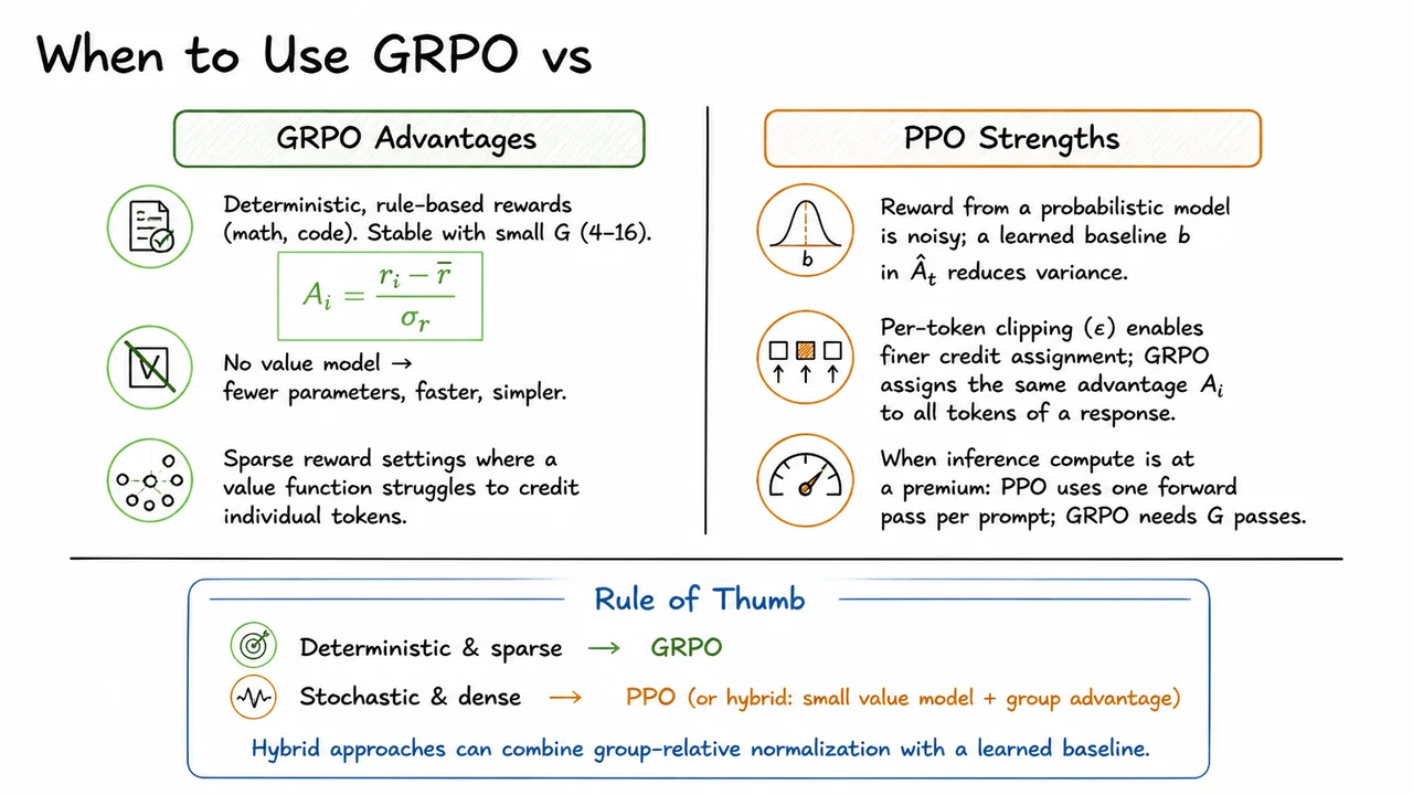
GRPO sidesteps the value function entirely. For each prompt it samples a group of complete responses, computes the scalar outcome reward for each response (e.g., 1 if the final answer matches the ground truth, 0 otherwise), then assigns the same group‑relative advantage to every token of response : where and are the mean and standard deviation of the rewards within that prompt’s group. This normalisation behaves as a crude approximate baseline: responses that score above the group average receive a positive update, those below receive a negative update, and the scale of the update is controlled by the within‑group dispersion. Because there is no separate value head to train, the implementation is simpler, the number of parameters grows more slowly, and there is no risk of value‑network collapse or overfitting. Empirically, for deterministic rewards like a math‑correctness checker, is remarkably stable even with a small (4–16), because the reward variance across responses is naturally small—most wrong answers are clearly wrong, and most correct answers are unambiguously right.
The trade‑off becomes clearer when we consider credit assignment. PPO can, in principle, vary the advantage per token if the reward model provides token‑level information or if the value function learns to predict intermediate goodness. More commonly, even with only a final scalar reward, the learned baseline acts as a “how good is this prefix” score, so tokens that lead to better completions are differentiated from those that do not. The per‑token clipping ratio in PPO’s surrogate objective further refines the update, preventing a single token from moving too far from the old policy regardless of the advantage magnitude. GRPO, by contrast, broadcasts the same advantage to every token of the response. If a response is successful overall, every token is reinforced equally; if it fails, all are penalised equally. This can be inefficient when some tokens are clearly responsible for the outcome—for example, an early logical mistake that dooms the rest of the answer—but in sparse, deterministic settings the outcome is often an all‑or‑nothing function of the final answer, so the uniform credit signal is not a major handicap.
Inference cost also tips the scales. PPO requires only a single forward pass per prompt during generation (the value network runs alongside the policy at a small extra cost). GRPO demands independent generations for each prompt, which multiplies the inference compute by . If generating a single long response is already expensive, this factor can be prohibitive. On the other hand, if inference is cheap and the reward signal is deterministic, GRPO’s group sampling can be amortised over the training run, and the rapid training (no value‑network updates) may still be competitive in overall wall‑clock time.
These characteristics lead to a simple decision heuristic: use GRPO when rewards are deterministic and sparse (math, code execution, structured output verification) and the extra inference cost is acceptable; use PPO, or a hybrid, when rewards come from a noisy probabilistic model (learned preference scorer, human feedback with high variance) or when token‑level credit is essential.
The visual below translates this reasoning into an at‑a‑glance decision guide. Its left column enumerates the key strengths that make GRPO appealing—no separate value model, stability with small groups, perfect fit for rule‑based rewards—while the right column highlights where PPO retains an edge: a learned baseline that tames noise, per‑token control via clipping, and lower inference overhead. At the bottom, a centred “Rule of Thumb” box offers the crisp takeaway: Deterministic & sparse → GRPO and Stochastic & dense → PPO / Hybrid. The diagram is not a prescriptive flowchart but a compact reminder that the best algorithm depends on the nature of the reward signal and the available resources, and it invites the practitioner to think about hybrids that could, for instance, combine a small value model with group‑relative normalization to get the best of both worlds.
The decision to use GRPO rather than PPO hinges on understanding what each algorithm removes, what it adds, and what it implicitly assumes about the reward landscape. After weighing the practical guidelines in the previous section, it is worth distilling the comparison into concrete, side‑by‑side contrasts that operate at the level of the training algorithm itself. Doing so reveals that the two methods differ not merely in implementation effort but in fundamental design principles—principles that echo early debates in reinforcement learning about value‑free policy gradients.
At the heart of the distinction is how each method estimates advantages. PPO, as typically deployed in RLHF, retains a learned value function to compute generalized advantage estimates (GAE):
This pipeline requires maintaining an extra model (the critic) and tuning the bias–variance trade‑off via . GRPO sidesteps all of that by exploiting group‑based relative advantages. For each prompt, the policy samples a batch of responses, each receiving a scalar reward from a (usually deterministic) reward function. No value function is needed because the advantage for response is computed by standardizing the rewards within the group:
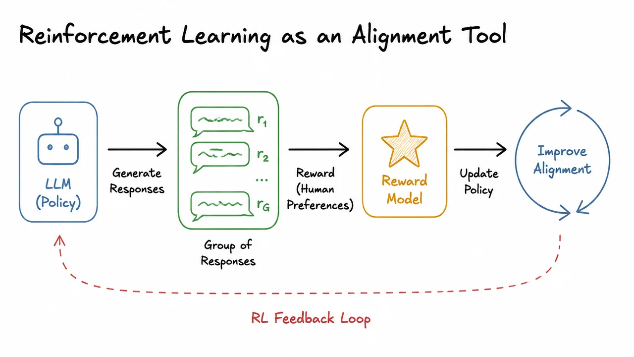
This simple formula already delivers a relative comparison: a response earns a positive advantage if its reward is above the group mean, negative otherwise. The scheme is reminiscent of policy gradient baselines that subtract the mean return but goes further by also normalizing with the standard deviation, which stabilizes training when reward scales vary across prompts. However, the normalization critically depends on the group statistics being informative. With deterministic, rule‑based rewards (common in math or code tasks) the group mean is a robust centroid; with noisy, learned reward models the standard deviation can become inflated and the advantage signal loses reliability. This is precisely why GRPO’s best‑case performance aligns with rule‑based settings, whereas PPO’s value‑function baseline can smooth out noisy reward signals over many episodes.
The presence or absence of a value model cascades through every other practical dimension. PPO’s critic reuses collected data to bootstrap value estimates, making it more sample‑efficient in terms of the number of forward passes through the policy per prompt. GRPO, on the other hand, must issue independent responses for each prompt and cannot share value information across prompts; this multiplies the number of forward passes, but the total computation may still be acceptable because a single forward pass through a large language model is often the dominant cost anyway. Implementation complexity tilts strongly in GRPO’s favor: one network, one loss function, no delicate tuning of the GAE parameters, and no risk of the value model diverging. PPO requires orchestrating the training of both policy and critic, managing the dual replay buffer, and often doubling the memory footprint—a burden that can be prohibitive for very large models.
These trade‑offs naturally map onto different use cases. When the reward signal is a learned preference model (as in RLHF), the implicit noise and drift make a learned baseline invaluable, so PPO remains the flexible workhorse. Conversely, when the reward is a compiler signal, an automatic math‑equality checker, or a unit test result, GRPO’s simplicity and stability become compelling. The compact comparison table that follows captures these contrasts at a glance. It lines up the two algorithms across the key dimensions—advantage source, extra model requirement, compatible reward types, sample efficiency, implementation complexity, and typical deployment scenarios—so that after reading the prose, you can quickly refresh the criteria that guide your choice. The takeaway line underneath the table, GRPO removes the value model by using group‑based relative advantages, offering a simpler and scalable alternative for rule‑based reward tasks; PPO remains more flexible when learned reward models are noisy, restates the central lesson in one sentence, exactly the kind of heuristic you want to carry into your next alignment project.