KV Caching in Autoregressive Transformers
1. Why Decoding Becomes Slow
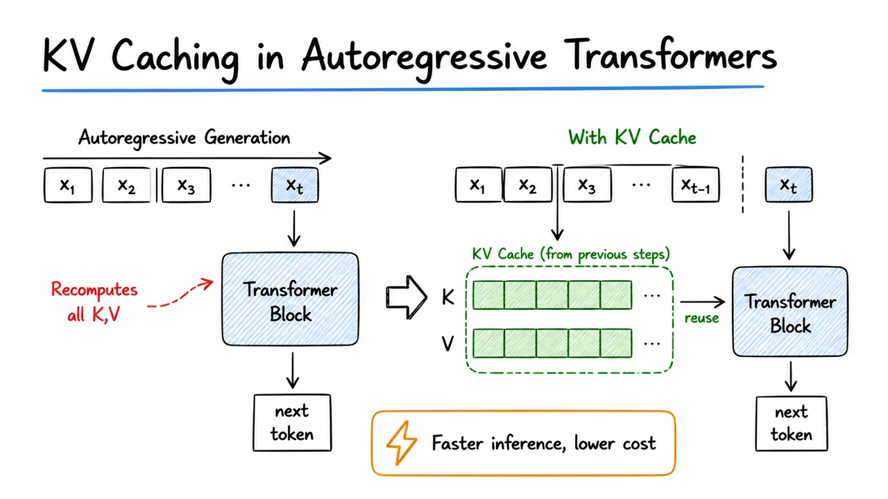
When a transformer is used for generation, the model does not predict an entire sequence in one shot. It advances one token at a time: at step , it consumes the prefix and produces a distribution for . That seems innocent enough, but it hides an important computational trap: if we run the transformer from scratch at every step, then every new token forces us to revisit all earlier tokens again.
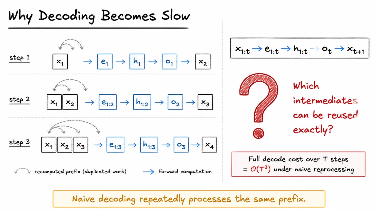
Formally, the decoding pipeline looks like Here are token embeddings, are the hidden states after the transformer layers, and is the output used to sample the next token. The problem is that most of this work for positions does not change when we move from step to step . Yet the naive procedure recomputes it anyway.
The key reason this becomes slow is that causal self-attention is prefix-based. For token , the hidden state depends on all earlier tokens . So when the prefix grows by one token, the model must produce the new hidden state for the fresh position, but under naive decoding it also rebuilds the representation of the entire prefix, including the same queries, keys, values, and intermediate activations that were already computed one step ago. In other words, the model is repeatedly paying for old context as if it were new.
This redundancy is easiest to see by comparing successive steps. Suppose we decode up to length . At step 1, the model processes a length-1 prefix. At step 2, it processes a length-2 prefix. At step 3, it processes a length-3 prefix, and so on. If the cost of processing a prefix of length scales roughly like because attention compares each token against all previous tokens, then the total cost over all decoding steps is That cubic growth is not a typo—it is the cumulative price of repeatedly reprocessing prefixes whose earlier parts are identical. In practice, constants and implementation details matter, but the asymptotic message is clear: naive decoding wastes a lot of compute on duplicated work.
There is a subtle but crucial distinction here. We are not saying the model’s output is redundant; each next-token prediction genuinely depends on the full prefix. The redundancy lies in the intermediate quantities used to obtain that output. If a tensor is a deterministic function of the prefix and the prefix has not changed, then that tensor should not need to be recomputed. This is exactly the opening for KV caching: we want to identify the internal states that can be reused exactly without altering the model’s answer.
The intuition becomes sharper if you think in terms of what attention actually needs. To score a new query against previous tokens, the model needs the previous tokens’ keys and values; it does not need to rebuild them from scratch every time. So the expensive part is not the mere act of appending one token, but the repeated reconstruction of everything the prefix already established. This is why decoding cost is dominated by prefix growth rather than by the one-token increment itself.
The visual below condenses that story into a compact sequence of three growing prefixes. Each panel shows the same earlier tokens reappearing, with faded looping arrows indicating that naive decoding revisits them again and again. The repeated blocks for embeddings, hidden states, and outputs are not there to suggest new computation; they serve as a reminder that the same pipeline is being run over an expanding prefix even though most of the prefix has not changed.
The red question mark is the real point of the slide: which intermediates can be reused exactly? Once we answer that, the whole decoding story changes. The next step is to separate what must be recomputed for the newest token from what can be stored and carried forward, turning repeated full-prefix evaluation into incremental inference.
2. Naive vs Cached Decoding
To see why KV caching matters, it helps to separate the mathematics of the model from the mechanics of decoding. In an autoregressive transformer, generating token requires predicting from the prefix . If we were to implement that naively, each new step would rerun the transformer over the entire prefix, even though almost everything in the prefix is unchanged from one step to the next. That is the core inefficiency: the model’s output at time depends on the same earlier context, but the implementation keeps rebuilding the same intermediate quantities again and again.
The expensive part is self-attention. For a query at position , the relevant output is
Notice what this equation actually needs: the new query , and the collection of past keys and values , . The earlier queries are not needed to compute . Yet in naive decoding, we still recompute them because the implementation typically processes the whole prefix through each layer from scratch. That means the same hidden states are repeatedly transformed into the same and over and over, even though these quantities do not change once token has been produced.
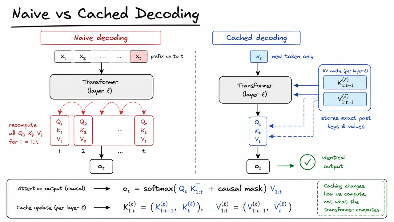
KV caching fixes exactly that redundancy. At step , we compute only the new activations for the fresh token : its query, key, and value at each layer. Then we append those to the stored prefix:
The important subtlety is that the cache stores exactly the past keys and values, not an approximation. So the transformer is not being changed into a cheaper model; it is the same model evaluated more efficiently. Because causal attention at position only looks backward, reusing the old and tensors gives the same that a full recomputation would have produced. In other words, caching changes how we compute, not what we compute.
That distinction is why KV caching is such a practical win. Without caching, decoding cost grows with the prefix length because each new token triggers redundant work over all earlier tokens. With caching, the work per step is concentrated on the new token and its interactions with the stored history. The tradeoff is straightforward:
- Less compute during decoding,
- More memory to store cached states for every layer and every past position,
- Identical outputs under the same model and causal mask.
This also explains a common failure mode: if you accidentally invalidate the cache by changing sequence order, switching batch composition, or applying a transformation that changes the hidden states, then the stored and no longer correspond to the current prefix. In that case, the outputs are no longer guaranteed to match naive decoding. So caching is only safe when the prefix and model state are exactly preserved; it is an optimization layer, not a mathematical shortcut.
The visual below condenses this idea into two parallel decoding graphs. The left side makes the redundancy visible: every new step reconstructs the full prefix and repeats the same projections over and over. The right side isolates the one genuinely new computation, while the cache box makes it obvious that earlier keys and values are simply being carried forward.
If you read the diagram as a comparison of work done rather than model behavior, the point becomes crisp: both paths end at the same attention output . The difference is that one path throws away previously computed state, while the other preserves it and reuses it. That is the entire logic of KV caching, and it is why the technique is now standard in production inference systems.
3. Self-Attention in Autoregressive Form
Building on the cached-decoding picture, the next step is to make the autoregressive attention rule completely explicit. Once we write the computation at a single time index , the caching story becomes almost inevitable: some tensors are ephemeral, because they are only needed to form the current output, while others are persistent, because future steps will reuse them verbatim.
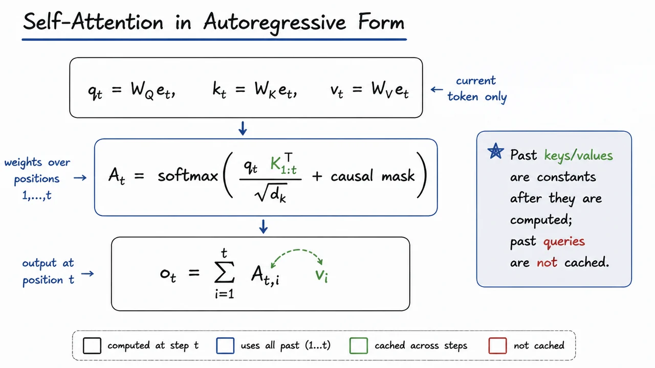
For a single-head causal attention layer, the current token embedding is projected into a query, key, and value: These three vectors play different roles even though they come from the same input. The query is the “question” posed by position ; the keys encode what each past position offers for matching; and the values are the information content that will be mixed into the output. In causal decoding, position is only allowed to attend backward, so the score for the current step is computed against the prefix keys , not the entire sequence.
The attention weights are then and the output is This is the crucial asymmetry: the query is consumed immediately to produce , while the keys and values are looked up repeatedly by every future query. Put differently, once and have been computed for a past token , they become read-only memory for the rest of decoding. There is no need to recompute them unless the model parameters change or the hidden state itself is being revised.
That asymmetry is exactly what makes KV caching correct. Caching does not alter the function computed by the transformer; it only stores the intermediate tensors that would otherwise be regenerated by reprocessing the same prefix. The model output remains identical because every future attention score still uses the same dot products , and every output still mixes the same values . What changes is the work schedule: instead of rebuilding from scratch at each time step, we append the newest to the cache and reuse everything else.
It is helpful to be precise about what can and cannot be cached:
- Cacheable: keys and values for each past token, because future queries will need them.
- Not cacheable in the same way: the current query , because it is only relevant for the current decoding step.
- Implicitly recomputed each step: the softmax weights , since they depend on the new query.
- Never reused directly: the output , because the next step will form a different output from a different query.
This also reveals a subtle failure mode: caching is only valid if the prefix representation is unchanged. If you drop tokens, change the prompt, rescale the sequence, or alter the hidden states through some nonstandard intervention, then the old keys and values no longer correspond to the current model state. In that case, reusing the cache would silently produce the wrong distribution. The correctness guarantee comes from a strict invariant: for every prefix token that remains in the context, its stored key and value must be exactly the ones the model would have recomputed.
From a computational standpoint, this layer-level decomposition explains why decoding without caching is so expensive. At step , naive autoregressive inference re-embeds the whole prefix and re-derives for all , even though only the newest query is needed to make the next prediction. Caching breaks that redundancy by turning the prefix into persistent memory. The tradeoff is obvious but important: we exchange extra memory bandwidth and storage for much less repeated matrix multiplication.
The visual below condenses that logic into a compact equation-centric view. The stacked formulas make the separation of roles visible: the top block shows the per-token projections, the middle block emphasizes that the attention scores are formed by querying the stored prefix keys, and the bottom block shows the weighted sum over cached values. The highlighted and are the tensors that survive across steps, which is exactly the part of the computation KV caching preserves.
4. A Two-Token Toy Example
Now that we have the autoregressive attention pattern in mind, the simplest way to see why KV caching matters is to shrink the problem to just two generated tokens. This toy setting is small enough to inspect by hand, but it already contains the essential redundancy that appears in long-form decoding.
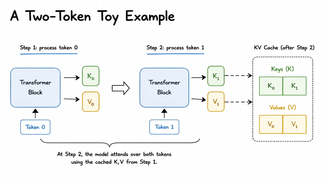
Suppose the model has already processed a prompt and produced hidden states for the first generated token, then it is about to generate the second one. In a naïve implementation, the model runs a full forward pass for the entire prefix again. That means the representations for token 1 are recomputed from scratch even though nothing about the earlier context has changed. The only genuinely new work is the contribution of token 2. Everything else is repeated arithmetic.
The key observation is that self-attention is asymmetric in decoding. When predicting the next token, the query for the current position must compare against all previous keys , but those earlier keys and values do not need to be recalculated. If the hidden state for token has already been computed once, then its projected key and value vectors can be stored and reused. In other words, for a single attention layer, each past token contributes two reusable objects: At the next step, we only compute the new query and append the new to the cache.
For two tokens, the contrast between naïve recomputation and cached decoding becomes almost embarrassingly clear. Without caching, the second step rebuilds the attention inputs for token 1 and token 2 together, even though token 1’s and are already known from the previous step. With caching, token 2 performs just one new projection into , then attends over the stored plus its own newly appended pair. The attention output is unchanged; only the amount of work differs.
This is the central compute-memory tradeoff. Caching reduces repeated matrix multiplications and avoids reprocessing the entire prefix, which is crucial because decoding is sequential and latency-sensitive. But the saved compute is bought with extra memory, since every layer must keep a growing record of past keys and values. For a two-token example the storage is tiny, but the scaling law is already visible: if each token adds one key and one value vector per layer, then memory grows linearly with generated length.
A subtle but important point is that the cache is not a generic shortcut for all transformer state. It works because causal self-attention only needs past keys and values to compute the next output. The queries are not cached in the same way, because a query is specific to the current position and is used immediately. That asymmetry is exactly what makes the optimization possible:
- Cache what is reusable: keys and values from previous positions
- Recompute what is position-specific: the current query
- Do not cache redundant activations unless a later layer truly needs them
Even in this minimal setting, a few failure modes are worth keeping in mind. The cache must stay perfectly aligned with the token order; if tokens are inserted, truncated, or reordered, stale entries will corrupt attention. Precision choices also matter: many systems store cached tensors in reduced precision to save memory, which is usually safe but can introduce numerical drift if the approximation is too aggressive. And in multi-layer transformers, each layer maintains its own cache, so a bug in one layer’s indexing can silently distort the whole generation process.
The visual below is useful because it condenses all of that into a single compact comparison. A two-token sequence makes the redundancy visible: the second step reuses token 1’s stored key and value rather than rebuilding them. That is the whole idea of caching in its smallest nontrivial form. Once that picture is clear, it becomes much easier to generalize to many tokens and many layers, where the same reuse pattern is repeated at scale.
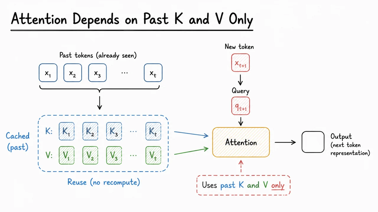
5. Attention Depends on Past K and V Only
After the two-token toy example, the broader pattern becomes easier to see: autoregressive self-attention does not need to revisit the entire hidden history as hidden states. What each new token really needs from the past is not the raw previous activations, but the keys and values produced from them. The query for the current position compares against past keys to decide where to attend, and then uses the corresponding past values to assemble the output. That separation is the core reason KV caching works.
For a single attention layer at time step , the computation is conceptually followed by attention over all earlier positions: The important asymmetry is that the new query depends only on the current token, while the keys and values from prior tokens are already sufficient summaries of what the model needs from the past. Once and have been computed for token , they can be reused for every later step. Recomputing them during decoding is mathematically redundant.
This is exactly where naive decoding wastes work. If you generate tokens one by one and, at each step, recompute attention over the whole prefix from scratch, then every previous token gets projected again into keys and values at every future step. The model is not learning anything new about those past tokens; it is merely redoing the same linear maps and the same memory reads. The redundancy is especially painful because attention cost grows with sequence length: at step , a naive implementation may pay work per layer just to rebuild information that was already known at step .
KV caching turns that observation into an implementation strategy. Instead of recomputing and , we store them and append only the fresh for the new token. The current query is still computed, and attention still scans over all cached keys and values, but the expensive projections for the old tokens disappear. In other words, the cache changes what is recomputed:
- naive decoding: recompute past and repeatedly,
- cached decoding: compute each token’s and once, then reuse them.
The subtle assumption here is that the model is strictly autoregressive and causal. That is what makes past keys and values immutable summaries: future tokens cannot alter them. If the architecture or decoding mode breaks that assumption—bidirectional attention, prefix edits, speculative rollbacks, or dynamic prompt rewriting—the cache can become invalid and must be refreshed or partially discarded. Caching is therefore not just an optimization; it is an optimization that relies on a very specific causal contract.
The same idea extends cleanly to multi-layer transformers, but with one important refinement: each layer has its own cache. The hidden representation entering layer at time differs from the one entering layer , so each layer produces distinct keys and values. During incremental decoding, the token’s representation is propagated forward through the stack once, and every layer appends its own new and to that layer’s cache. This is why production systems often speak of a “KV cache” as a collection of per-layer tensors rather than a single global memory.
The payoff is large, but so is the memory footprint. Caching trades compute for memory: you avoid repeated matrix multiplications, but you must keep all cached keys and values resident for the active context. For long contexts, batch decoding, or large models, this becomes the dominant inference cost. In practice, the cache is often the bottleneck before arithmetic is. That tension explains why systems engineers care so much about layout, precision, paging, quantization, and eviction policies: they are all attempts to keep the cache usable without letting it dominate device memory.
There are also practical failure modes that are easy to miss if you only think in equations. A cache must stay aligned with the exact token sequence used to produce it; any mismatch in tokenization, truncation, beam branching, or prompt editing can silently corrupt generation. Mixed precision can introduce small numerical differences, and multi-request batching can complicate how cached entries are packed and indexed. So the conceptual rule “attention depends only on past and ” is simple, but the systems rule is stricter: the cache must faithfully represent the exact causal history for each layer and each sequence position.
The visual below condenses that logic into a compact diagram: the current token produces a fresh query, while the past contributes cached keys and values that are simply reused. That makes the causal dependency explicit without redoing the entire derivation. It is also a useful bridge to the next idea, because once you accept that only the newest token needs new projections, the remaining question is how to write the recurrence so decoding can advance one step at a time with minimal recomputation.
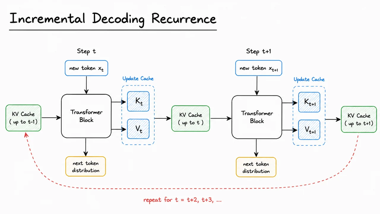
6. Incremental Decoding Recurrence
Once we accept that, during autoregressive generation, the model only needs the past keys and values, the next question is how to turn that observation into a usable recurrence. The answer is simple in spirit: instead of recomputing the entire prefix at every step, we treat decoding as a stateful process. At time step , the model consumes the new token , produces its query , and appends the newly computed key and value to a growing memory of all earlier positions. The recurrent state is therefore not a hidden vector in the RNN sense, but a pair of tensors containing all prior attention ingredients.
For a single attention layer, this gives a very compact update rule. If and are the cached key and value matrices for the prefix, then decoding step forms The new query attends against this expanded cache to produce the output at position . The key point is that the recurrence is append-only: nothing from earlier positions changes, so previously computed projections can be reused exactly. This is why incremental decoding avoids the quadratic waste of naive recomputation, even though the final attention result at each step is the same.
The subtlety is that this recurrence is not a magical shortcut around attention itself; it is a bookkeeping identity. The expensive part of standard decoding is that when we generate token , a naive implementation re-derives and from scratch even though those tensors depend only on old tokens. With caching, the per-step work changes from “reprocess the whole prefix” to “project one new token and perform one new attention query.” In other words, the compute drops from repeatedly revisiting the past to merely reading the past.
This also makes the memory tradeoff explicit. A cache saves FLOPs because it stores the prefix activations, but it costs memory proportional to sequence length. For one layer and one sequence of length , the cache stores roughly numbers for keys and another for values, where is the head dimension times the number of heads, up to implementation details. In practice, the hidden cost is not just raw bytes; it is also bandwidth. During decoding, each new token must stream through all cached and , so long contexts can become memory-bound even when arithmetic is cheap.
The recurrence becomes more interesting in a multi-layer transformer. Each layer has its own key-value cache , because the inputs to layer depend on the outputs of layer . So the update happens layer by layer:
- compute the new hidden state at layer ,
- project it into ,
- append those tensors to that layer’s cache,
- move upward to the next layer.
This is why production systems often describe KV caching as a stack of per-layer memories rather than one global buffer. The recurrence is simple, but it must be applied consistently across layers, heads, batch elements, and variable-length sequences. Any mismatch in indexing or masking breaks exactness immediately.
There are also important failure modes to keep in mind. Caching is exact only when the model’s past computations are unchanged. If you alter the prefix through editing, speculative rollback, beam search pruning, prefix sharing, or certain forms of positional remapping, the cache may become invalid or require careful reindexing. Similarly, implementation bugs often come from off-by-one errors in the causal mask, incorrect token alignment, or reusing a cache across sequences that no longer share the same prefix. The recurrence is mathematically straightforward, but operationally it is unforgiving.
That is why incremental decoding is best understood as the bridge between theory and deployment. The transformer is still computing the same causal attention function, but it does so in a streaming way that exposes the algorithmic structure of generation: append one token, update one layer after another, and never revisit what the model already knows. The visual below compactly organizes that logic into a single left-to-right flow, so you can see the cache growing step by step rather than imagining attention as a full recomputation at every token.
It also helps separate the two layers of meaning in the recurrence. The arrows capture the dataflow of a new token through the network, while the cached blocks summarize the persistent state that survives across time. That distinction is exactly what makes KV caching useful: the visual memory of the past is not the whole prefix re-run, but the minimal sufficient state needed to make the next causal attention computation exact.
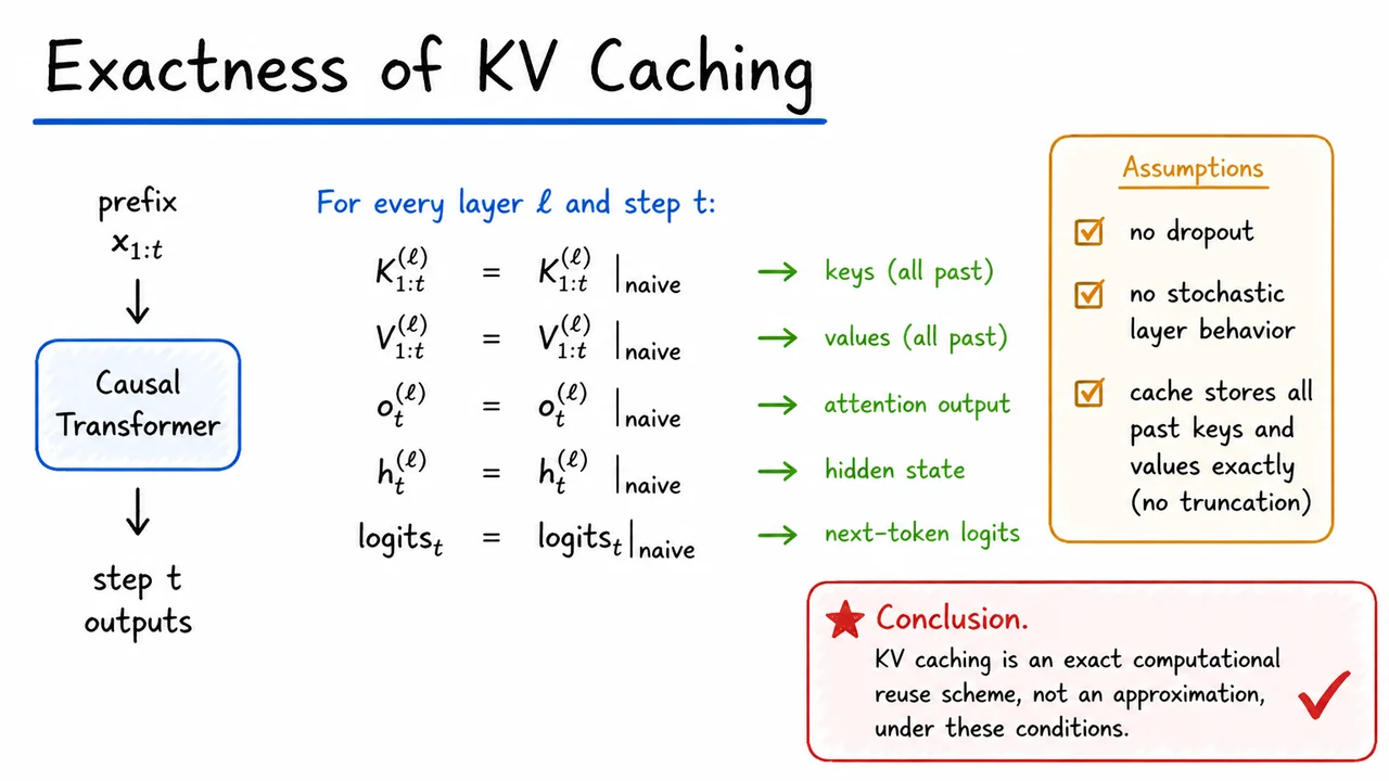
7. Exactness of KV Caching
After the recurrence for incremental decoding, the natural question is whether the cache is merely a speed trick or something deeper. The answer is surprisingly strong: if we store every past key and value exactly, caching does not change the model’s computation at all. It only changes how we arrive at the result. The transformer still evaluates the same causal function on the same prefix ; it simply avoids redoing work that was already determined at earlier steps.
The cleanest way to state this is as an equality of internal states. For each layer and time step , the key and value tensors produced by cached decoding match those from naive recomputation on the entire prefix: Once those match, the rest of the network follows by causality. The attention weights at step depend only on the query at and the stored past keys, so the attention output must match as well: In other words, exactly the same prefix, exactly the same parameters, exactly the same output.
What makes this work is the transformer’s causal structure. At step , the computation of the representation for position does not depend on future tokens, only on . The cached algorithm preserves this dependency graph: past positions contribute only through their already-computed keys and values, while the new token contributes a fresh query, key, and value. There is no approximation hiding in the reuse. If the cache contains the full history, then the cached run and the naive run are two ways of evaluating the same recurrence.
This exactness relies on a few subtle assumptions that are easy to gloss over in implementation but crucial in theory:
- No dropout or stochastic layers during inference.
- No cache truncation, eviction, or compression.
- No numerical perturbation beyond the usual deterministic arithmetic of the chosen backend.
- Fixed parameters and identical tokenization / positional encoding conventions.
Once any of these are relaxed, exact equality can fail. Truncating the cache changes the function being computed; approximating keys or values changes the attention logits; stochastic inference introduces randomness that can break step-by-step equivalence. So the theorem is not saying that “all caching methods are exact,” but rather that full, faithful KV caching is exact.
This distinction matters because it tells us how to reason about inference correctness. The cache is not part of the model in the semantic sense; it is a memoization mechanism for intermediate tensors. That means we can use the cached algorithm to accelerate decoding without changing the model’s output distribution, provided we preserve the full causal state. The practical payoff is enormous: we replace repeated recomputation over the prefix with incremental updates, while keeping the same logits, the same generated tokens, and the same layerwise activations.
It is also worth noticing what exactness does not claim. It does not say the cached version is cheaper in every dimension; it trades compute for memory. Nor does it say the cache is robust to every engineering shortcut. Quantization, sliding windows, speculative cache eviction, and paged or compressed variants may be very useful in production, but they are no longer the same theorem. They introduce controlled approximations or altered execution rules, and then exactness has to be re-evaluated separately.
The visual below compresses this idea into a compact theorem-style summary: the central equalities assert that the cached and naive tensors coincide, while the boxed assumptions remind us why the proof goes through. The small conclusion “Cache = exact reuse” is intentionally terse, because that is the conceptual endpoint of the argument: caching is not changing the computation, only avoiding redundant work.
Seen this way, the diagram is not a replacement for the proof; it is a mnemonic for it. The equalities in the center encode the inductive invariant we will use next, and the assumptions box marks the boundary between exact theory and approximate systems engineering.
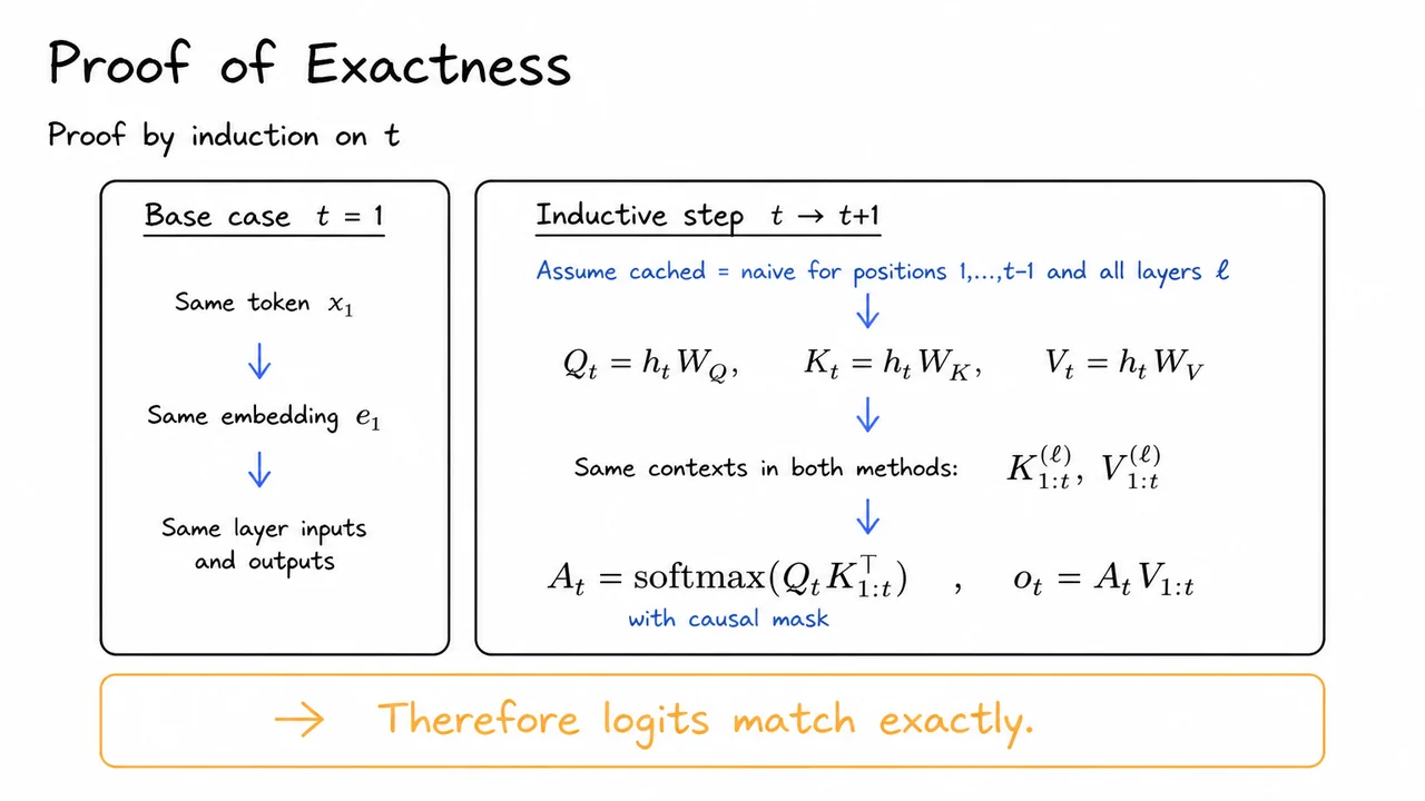
8. Proof of Exactness
We are now ready to turn the informal intuition into an actual proof. The key claim is stronger than “caching seems to work”: it says cached decoding is exactly equivalent to naive recomputation at every decoding step, so long as we are comparing the same model, the same parameters, and the same causal mask. In other words, caching is not an approximation to autoregressive inference; it is a reorganization of the same computation.
The cleanest way to prove this is by induction on the decoding step , with a nested argument over layers . That structure matches the computation graph of a transformer: each new token is processed by the stack one layer at a time, and each layer depends only on the current hidden state and the accumulated past keys and values. The proof therefore needs to show that if all earlier prefixes were processed identically, then the next step also stays identical.
Start with the base case . Both naive recomputation and cached decoding begin from the same first token , so they form the same embedding , the same layer input, and therefore the same hidden states, keys, values, and logits. There is no room for divergence yet: the cache is either empty or freshly populated, but in both implementations the first forward pass is the same function of the same input. This base case matters because it anchors the entire induction in a concrete shared state rather than a bookkeeping assumption.
Now assume the inductive hypothesis: for all positions and for every layer , the cached and naive methods have produced identical hidden states. Equivalently, the stored key and value tensors for the prefix are identical in the two implementations. This is the only nontrivial assumption we need, and it is exactly what makes caching safe: the cache is not allowed to invent new activations or stale ones; it must simply preserve the ones that naive recomputation would have produced.
At step , both methods receive the same current layer input . Therefore their linear projections agree: This is where the proof becomes almost mechanical. Since the current token’s hidden state is the same, the query, key, and value generated from it are the same. Combined with the inductive hypothesis that all previous and entries also match, both implementations assemble the same causal attention context.
That means the attention weights are identical: The causal mask is doing important work here. Without it, future positions could influence the attention distribution, and the stepwise equivalence would fail because the “current” computation would depend on tokens that have not been generated yet. Under the causal constraint, however, the output at time depends only on the shared prefix and the current token’s own projections, which are equal by construction.
Once the attention output matches, everything downstream in that layer matches as well: residual connections, normalization, feedforward transformations, and then the next layer’s input. So the argument repeats layer by layer. This is why the proof is naturally phrased as an induction over inside the induction over : equality at one sublayer propagates forward through the remainder of the stack, and equality at the final layer gives the same next-token logits.
The practical conclusion is simple but powerful:
- Same inputs same projections
- Same stored prefix same attention context
- Same attention output same hidden states
- Same hidden states same logits
So the cache changes how we evaluate the model, not what function the model computes. That is why KV caching can be trusted in production inference systems: it removes redundant work while preserving exact autoregressive semantics.
The visual below is a compact version of this proof. The base-case box anchors the induction at , while the inductive-step box shows the chain of equalities that carries the argument forward: identical hidden state, identical , identical causal context, identical attention output, identical logits. Read as a proof sketch, the diagram is not merely decorative; it is evidence that the cached path and the naive path are computing the same mathematical object in two different ways.
9. Multi-Layer, Multi-Head Cache Layout
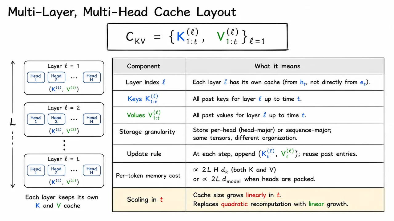
Building on the exactness argument, the key point is that a cache is not a single shared memory for the whole transformer. It is a layerwise collection of per-token key and value tensors, because each layer transforms the representation before producing its own attention projections. In other words, the cache must preserve exactly the information each future attention computation will need, and that information is different at every depth.
Formally, for a sequence observed up to time , the cache is This notation matters: the superscript reminds us that layer owns its own history, while the subscript says we keep all past positions. The cache is therefore not “the last hidden state,” nor a compressed summary of the prefix; it is the complete set of keys and values that causal attention may query later.
A subtle but important assumption is that the keys and values at layer are computed from that layer’s hidden states , not directly from the token embedding . So if we want exact decoding, we cannot reuse one layer’s cache for another layer, even if the same token is being processed at the same timestep. Each layer has a different representation space, a different query, and therefore a different set of attention logits: If we changed or omitted any past or , we would change the attention output and break exactness.
With heads, each layer’s cache is really a stack of head-specific tensors. One can store this in head-major form, where the head index is contiguous, or in sequence-major form, where time is contiguous. These layouts are implementation choices, not mathematical ones: they contain the same tensors arranged differently. That distinction becomes important in practice, because memory coalescing and kernel design depend on layout, but the underlying object remains the same per-layer cache.
The update rule is simple but powerful: when a new token arrives, compute once for every layer , append them to the layer’s cache, and reuse everything older without recomputation. This is the whole reason KV caching changes decoding from repeated quadratic work to linear growth in sequence length. Instead of recalculating all past projections at step , we pay only for the fresh token.
The tradeoff is memory. Since every token contributes both keys and values in every layer and head, the storage cost grows like or equivalently when the head dimensions are packed into the model dimension. The factor of 2 comes from storing both and ; the factor of comes from one cache per layer; the factor of is the per-layer projection width across heads. This is why production systems often talk about KV cache bandwidth and capacity as first-class constraints: the cache is what makes fast decoding possible, but it is also what consumes most of the memory.
The practical takeaway is a clean one:
- Exactness requires preserving every past key and value.
- Layerwise separation is unavoidable in multi-layer transformers.
- Multi-head storage can be reorganized, but not reduced without approximation.
- Linear growth in is the price of avoiding repeated recomputation.
The visual below is a compact way to make those abstractions concrete. The stacked layers emphasize that each layer owns its own cache, while the table organizes the same idea from two angles: what is stored, and why it scales the way it does. The key/value color split reinforces that both are necessary, and the final row makes the central engineering fact impossible to miss: caching saves compute by trading it for memory that grows linearly with sequence length.
10. Layerwise Cache Update in a Tiny Transformer
Once we move from the abstract cache definition to an actual decoder, the key question becomes: what exactly changes when the next token arrives? The answer is deceptively simple, but it is the entire mechanism behind efficient autoregressive inference: a new token does not refresh one global store, it extends a separate cache inside each layer.
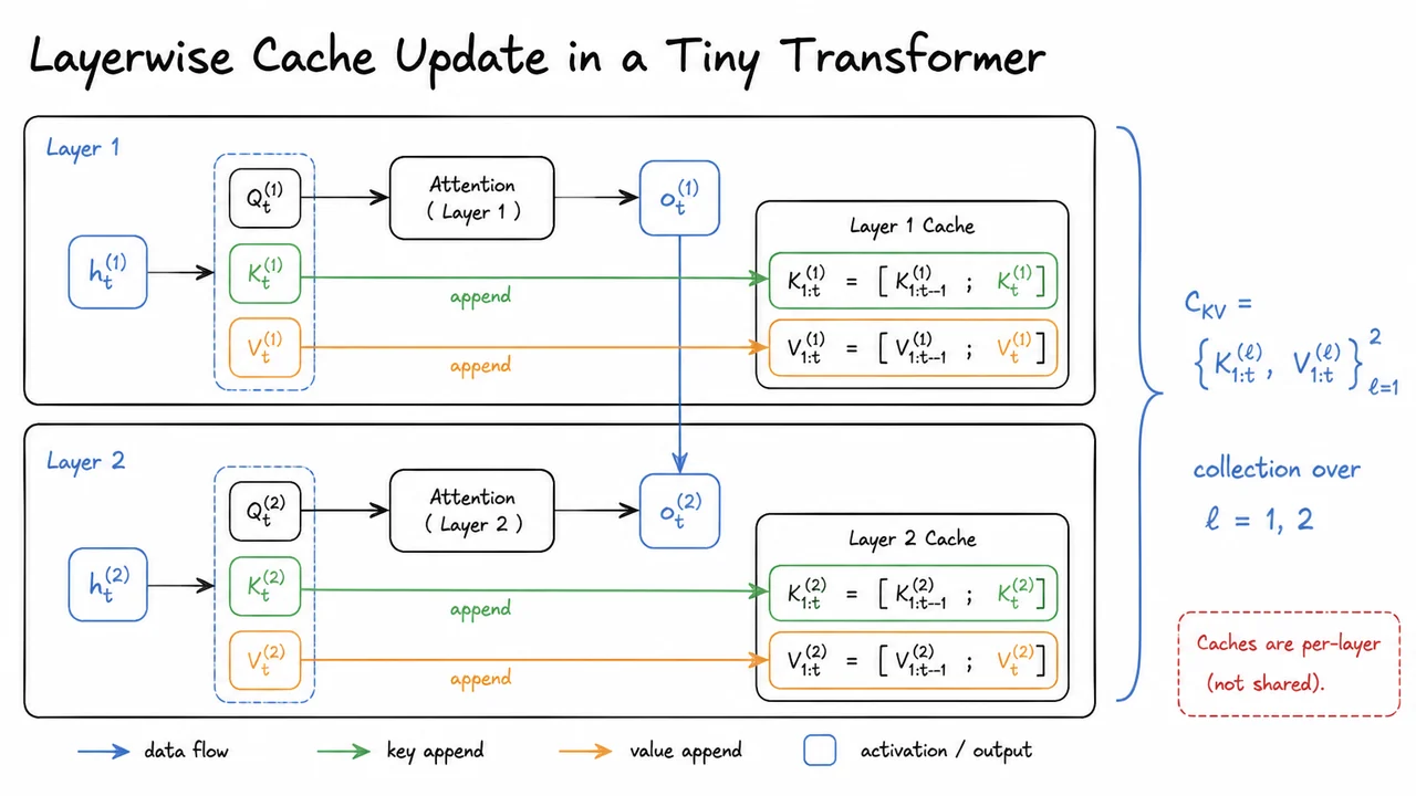
Consider a tiny decoder with two layers. At decoding step , layer 1 sees its own layer input and produces the usual projections . The new key and value are then appended to the layer-1 cache, Nothing exotic is happening here: the cache is just an append-only history of what this layer has already computed for earlier tokens. The crucial point is that this history belongs to layer 1 only.
That layer-specific cache is then used to compute the current attention output, This is the usual causal attention formula, except now the matrix multiplication only needs the cached past keys and values rather than a full recomputation over the whole prefix. In other words, caching changes what gets stored, not the mathematics of attention itself. The decoder still attends over all previous positions; it simply reuses the previously computed and tensors instead of rebuilding them from scratch.
The output is then passed upward as the input to layer 2, where the same logic repeats with different parameters and a different hidden state . So layer 2 forms its own , appends them to its own cache, and computes its own attention output from that local store. The same token index appears in both layers, but that does not mean the stored tensors are shared. Each layer has its own evolving sequence of keys and values because each layer has its own representation space.
This is the subtle failure mode that often trips people up: if you imagine a single cache for the whole model, you implicitly assume that a key produced in one layer could be reused in another. But keys and values are layer-dependent projections of different hidden states, so they are not interchangeable. A cache is only valid for the layer that created it. That is why the full decoder cache is best written as the collection which is really a stack of independent append-only stores, one per layer.
A few practical consequences follow immediately:
- Updates are local: when token arrives, every layer appends exactly one new key and one new value to its own cache.
- Reuse is layerwise: decoding at step can reuse the entire prefix, but only within the same layer.
- No cross-layer sharing: the cache is not a single tensor bank; it is a family of per-layer histories.
The visual below is useful because it compresses this logic into a tiny two-layer decoder. It makes the independence of the two caches obvious: the same token index flows through both layers, yet each layer performs its own projection, appends to its own and , and computes attention from its own stored history.
It also highlights why the cache is described as append-only. Nothing in the past is rewritten; the model just adds one more row to each layer’s key/value store. That simple invariant is what makes incremental decoding correct, efficient, and easy to reason about when we later compare the compute saved by caching against the memory it consumes.
11. Compute vs Memory Tradeoff
Once we cache keys and values, the central question stops being whether decoding is faster and becomes what we pay for that speed. Autoregressive generation is a streaming problem: at time step , the model only needs the next token, but it must still attend over all previous tokens . Without caching, every new token would force us to recompute the full key and value projections for the entire prefix, even though those prefix states have not changed. The cache removes that redundancy, but it does so by storing intermediate activations in memory instead of recomputing them in compute.
That exchange is easiest to see in the attention cost. For a single layer with hidden size , each new token produces a query, key, and value. In naive decoding, the model repeatedly forms and from scratch for every step, so the work for prefix tokens is paid over and over again. With caching, the computation for an old token is done exactly once, and only the new token’s and are appended. The attention score computation still scales with context length because the new query must compare against all cached keys, but the expensive linear projections over the prefix disappear.
This gives a very clean tradeoff:
- Compute decreases because we avoid redundant and projections for past tokens.
- Memory increases because we must retain all cached and tensors for every layer and every generated token.
- Latency improves most during decode, when sequence length is growing one token at a time and recomputation would otherwise dominate.
- Memory pressure grows linearly with context length, number of layers, and batch size.
A useful way to think about it is that caching turns attention into a classic time-for-space optimization. The model pays a one-time cost to store enough information to make future steps cheap. If the cache were free, this would be a pure win. In practice, the cache becomes the dominant memory consumer in long-context inference, especially for large models with many layers and wide heads. For a batch of requests, the total KV footprint can quickly rival or exceed the model weights themselves.
For a multi-layer transformer, this tradeoff compounds. Each layer has its own key and value tensors, so the cache is not a single buffer but a stack of per-layer histories. If layer stores keys and values of shape roughly , then over layers the memory scales like with the factor of 2 coming from keys and values. The exact constant depends on dtype and layout, but the important point is the same: longer contexts are not just more compute, they are more memory. That is why practical systems often care as much about cache layout, paging, and eviction as they do about raw FLOPs.
The failure mode here is also instructive. If the cache is too large for device memory, decoding can stall, spill, or force smaller batch sizes, which may erase the throughput gains from caching in the first place. If the cache is aggressively compressed or truncated, the model may lose long-range information and degrade quality. So KV caching is not an unconditional optimization; it is a budget allocation problem where compute, memory, and fidelity are all coupled.
This is also why production inference systems distinguish between different cache variants. Some systems use static preallocation for predictable shapes, others use paged or block-based caches to reduce fragmentation, and some apply quantization or precision reduction to lower the memory footprint. Each variant changes the balance slightly: less memory per token usually means more bookkeeping, more irregular access, or a small accuracy risk. The best choice depends on whether the bottleneck is bandwidth, capacity, or latency.
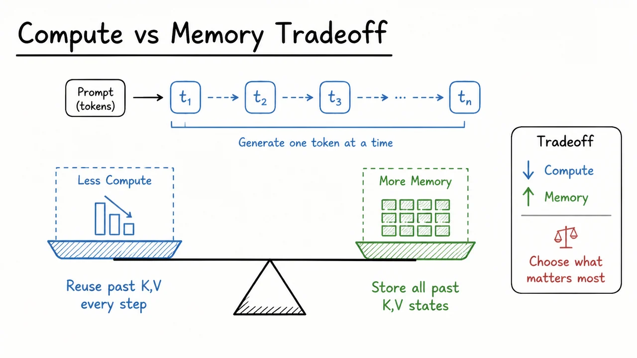
The visual below is useful because it compresses that balance into a single picture: the left side emphasizes repeated compute when we do not cache, while the right side emphasizes the growing memory footprint when we do. That contrast is the real lesson. KV caching is not merely an implementation detail; it is the mechanism that shifts autoregressive decoding from redundant recomputation toward a memory-resident incremental algorithm.
Seen this way, the diagram is not just illustrating an efficiency trick. It is summarizing the core systems insight of transformer inference: decode speed is bought with state retention. Once that mental model is clear, the next step is to measure how much of the benefit survives in practice, which is exactly where prefill versus decode benchmarks become informative.
12. Micro-Benchmark: Prefill vs Decode
After we understand the asymptotic story, the next question is more practical: where does the wall-clock time actually go during generation? In an autoregressive transformer, a serving system almost never spends all of its time in one homogeneous phase. It spends a large, parallelizable burst of work on the initial prompt, and then a much longer sequence of small, sequential steps while tokens are emitted one by one. That split is exactly what makes KV caching operationally useful, because it separates the expensive construction of context from the cheap reuse of it.
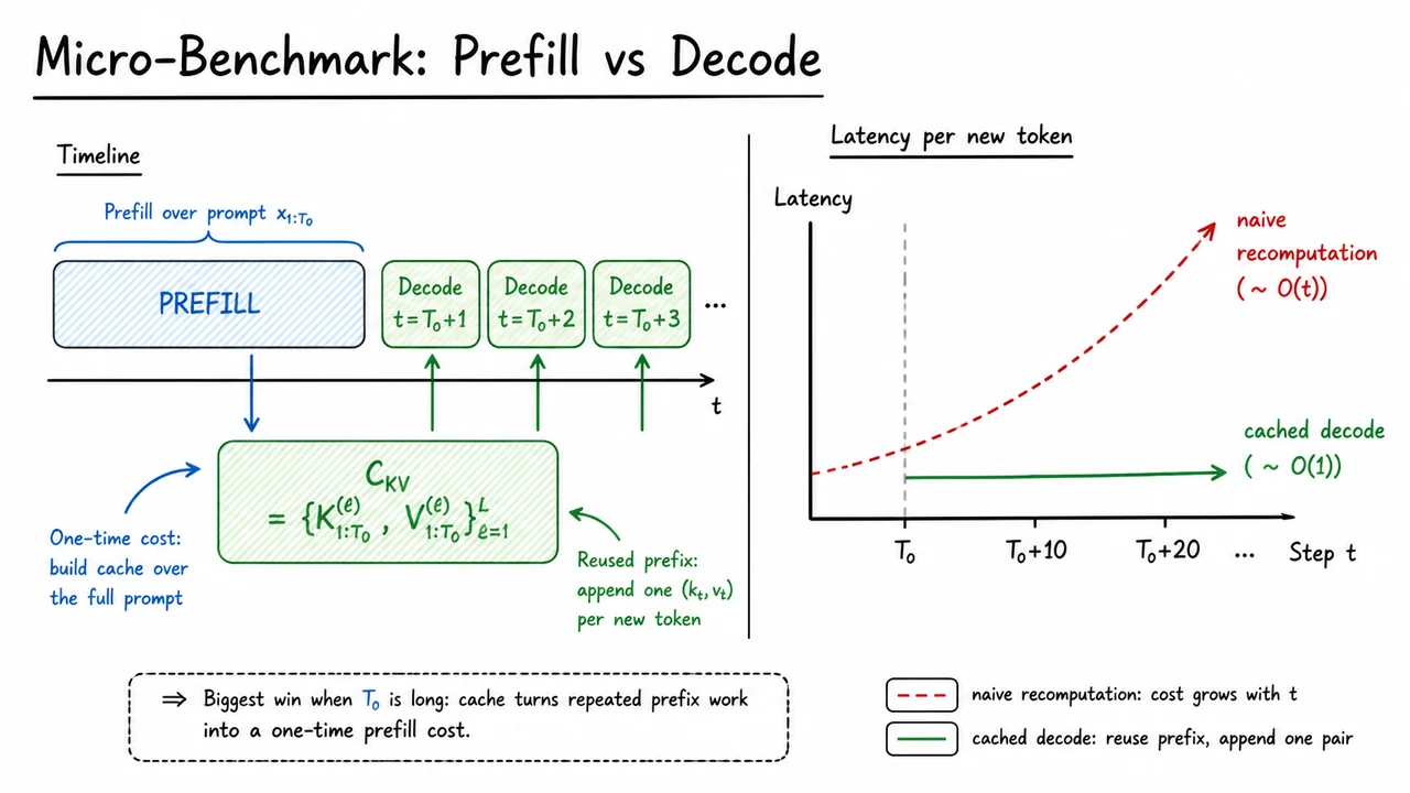
The key idea is to treat inference as a two-phase pipeline. During prefill, the model reads the prompt in parallel and computes all per-layer key and value tensors for that prefix. Collecting these tensors gives the cache This object is not just an optimization detail; it is the state that lets decoding avoid reprocessing the entire prompt at every step. Once the prefix has been encoded, every future token only needs the new query and the cached prefix keys and values.
That means the attention computation changes shape. Instead of re-evaluating all prefix projections and attention scores from scratch, we compute where the cache supplies and , and we append the new pair after processing the current token. The subtle but important point is that the attention itself is still exact; caching does not approximate the model. It simply avoids recomputing the prefix projections and the prefix contributions to attention.
This is why the compute profile changes so dramatically. In the naive implementation, step attends over an ever-growing prefix and also pays to rebuild all of that prefix state, so the work per step scales like . With caching, the incremental update is effectively for the new cache entries, while the remaining attention over the stored prefix is limited to the unavoidable lookup and scoring against existing keys. In practice, that makes decode sequential but stable, whereas naive recomputation becomes increasingly expensive as the generated sequence grows.
A useful way to think about the benchmark is as a micro-economy of latency:
- Prefill: high work, high parallelism, one-time cost.
- Decode: low per-step work, low parallelism, repeated many times.
- Naive recomputation: pays the prefill-like cost again and again.
- Cached decode: pays once, then reuses the prefix.
This tradeoff also explains why cache benefits grow with prompt length . If the prompt is short, the one-time prefill is not especially expensive, and the savings from caching are modest. But when the prompt is long, repeated prefix recomputation dominates the naive path, so turning that repeated work into a single prefill pass yields a large throughput win.
There is an important systems nuance here: the prefill phase is usually compute-heavy but highly parallel, while decode is sequential but cache-efficient. That means a benchmark that reports only total tokens per second can hide the real bottleneck. If you want to understand serving latency, you need to separate the two regimes, because the same model can look fast in aggregate yet still feel sluggish when prompt processing or per-token decode is the limiting factor.
The visual below is a compact summary of that story. The left side captures the pipeline view: a long prefill block over the prompt, a shaded cache that stores the prefix state, and then a chain of decode steps that reuse that prefix rather than rebuilding it. The right side turns the same idea into a latency sketch: the naive curve rises with step index, while the cached curve stays much flatter. Together they make the central message concrete — KV caching does not remove the sequential nature of generation, but it converts repeated prefix work into a one-time cost.
13. Implementation Details That Matter
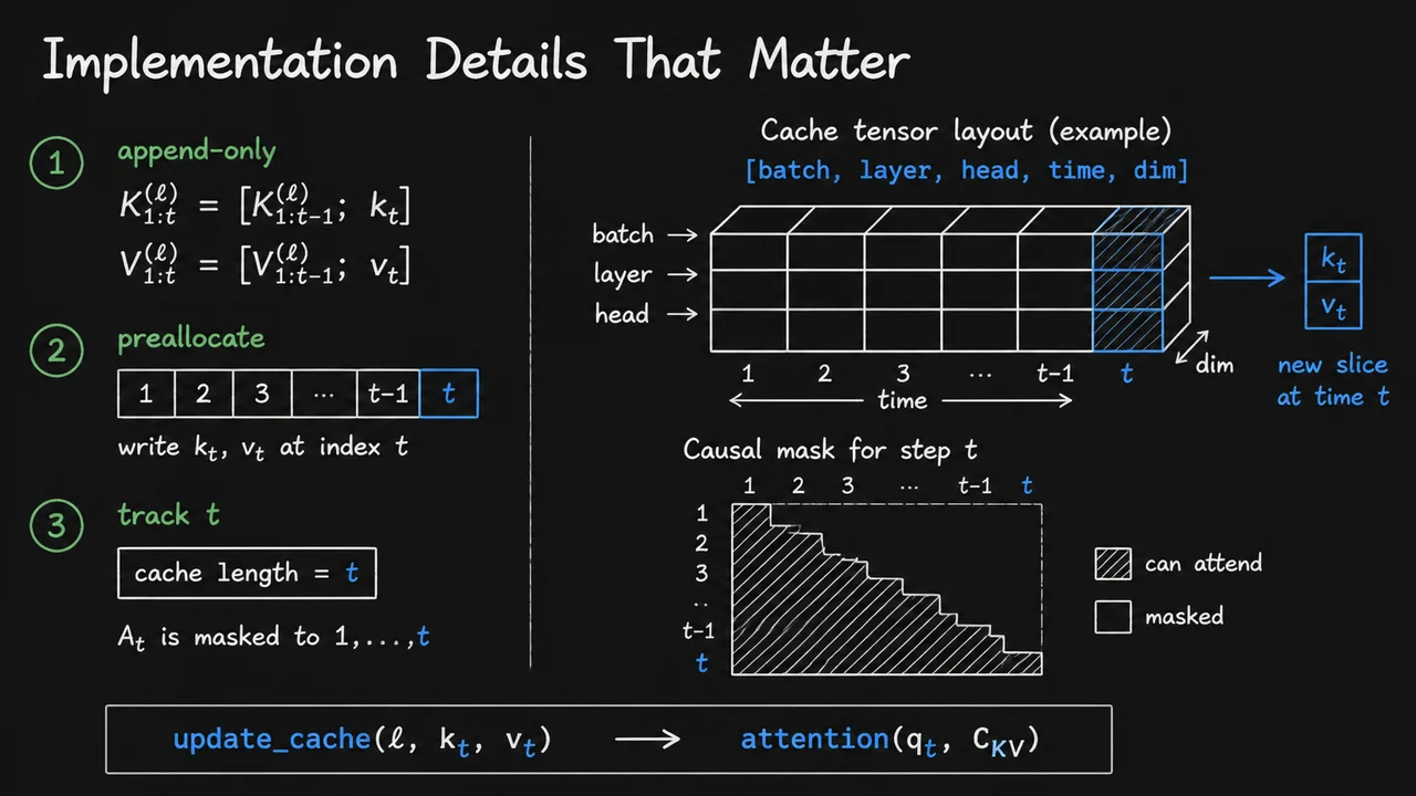
Building a KV cache into a decoder is not conceptually difficult, but the implementation details are what decide whether the idea becomes a speedup or a source of bugs. The mathematical update is simple: at step , each layer appends the newly computed key and value to its running prefix, What makes this practical is that the cache is append-only from the model’s point of view: past entries are never rewritten, because their values already correspond to earlier positions and earlier queries. If we were to recompute them every decoding step, we would lose the whole point of caching; if we were to mutate them in place incorrectly, we would silently break equivalence with the original autoregressive model.
The first design choice is whether the cache grows dynamically or lives in a fixed block of memory. In an append-only growth implementation, each step concatenates the new and onto the existing tensors. This is straightforward conceptually, but naïve concatenation can be expensive if it triggers repeated reallocations or copies. In a fixed-capacity preallocation scheme, the system reserves a tensor of maximum length up front and simply writes the new slice at index . That version is usually preferred in production because it makes memory usage predictable and avoids fragmentation, but it requires the model to know or bound the maximum decode length.
The cache length itself is not implicit; it must be tracked explicitly. At step , the valid prefix length is and the causal attention mask must agree with that fact. The query at position is allowed to attend only to positions , never beyond them. This sounds obvious, but it is one of the easiest places to introduce an off-by-one bug: if the mask is built for the wrong length, the model may either attend to uninitialized memory or incorrectly hide a valid token. In other words, the cache and the mask are a coupled pair; changing one without the other breaks the decoder’s semantics.
The memory layout also matters more than it first appears. A typical cache tensor is arranged as , or a close variant of it, because decoding repeatedly reads past keys and values along the time dimension. That layout is chosen for locality: the model does not need to scan the whole tensor structure to find the next token’s history. Instead, it can stream through the cached prefix in a way that is friendly to batched GPU kernels. The main tradeoff is familiar from systems work:
- better locality and throughput usually require more careful layout choices;
- more flexible tensor abstractions are often easier to write, but slower to execute;
- fixed-dimensional cache blocks are efficient, but demand disciplined indexing.
Another subtle but crucial point is that positional information is applied when , , and are formed, not by modifying stored cache entries later. Once a key or value has been written into the cache, it should represent the exact transformed feature vector for that time step. If the model uses rotary embeddings, learned position embeddings, or another positional scheme, those transformations are baked into the tensors before caching. Trying to “fix up” positions afterward introduces consistency issues, especially in multi-layer settings where each layer’s cached representation must remain aligned with the layer’s own attention computation.
That is why production code often looks like an update-and-read pipeline rather than a pure function from token to output. A useful mental model is The cache is updated first, and then the current query reads the stored prefix. This sequencing matters because the attention computation at step must see the latest prefix , including the newly generated token if the implementation includes self-attention over the current position. Getting this order wrong can produce subtle semantic shifts that are hard to detect from speed benchmarks alone.
The visual below compresses all of those moving pieces into one layout. The left side summarizes the three operational choices that govern a real decoder: whether the cache grows by append, whether memory is preallocated, and whether a separate counter tracks the current length . The right side makes the memory picture concrete by showing the 5D cache block, the highlighted time axis, and the new slice being written into position . The small causal triangle is there to reinforce the masking rule: the model may only read the prefix that has actually been built.
Read together, the diagram and the update rule make the same point from two angles. The equation tells you what must happen mathematically; the tensor sketch tells you how it is made to happen in a real system. That connection is the whole lesson of implementation detail: caching is not just about storing past activations, but about storing them in a layout, order, and mask discipline that preserves autoregressive correctness while making decode fast enough to matter.
14. Common Cache Variants and Failure Modes
After we understand the basic cache idea, the next question is not whether to cache, but what exactly to cache and when the cached state can stop being valid. In practice, real inference systems rarely use a single “canonical” cache. They choose among several variants that trade memory, flexibility, latency, and implementation simplicity in slightly different ways. That is where many of the subtle bugs live.
The baseline scheme is straightforward: during autoregressive decoding, each new token only needs to attend to the prefix that came before it. Instead of recomputing the entire prefix attention at every step, we store the previously computed keys and values and append the new ones. For a single layer with sequence positions , we keep and at step we compute only the new , then form attention against the cached prefix. In a multi-layer transformer, this becomes a per-layer cache: each layer stores its own and . That layered separation matters because the hidden states differ by layer, so there is no single shared cache that can be reused across all blocks.
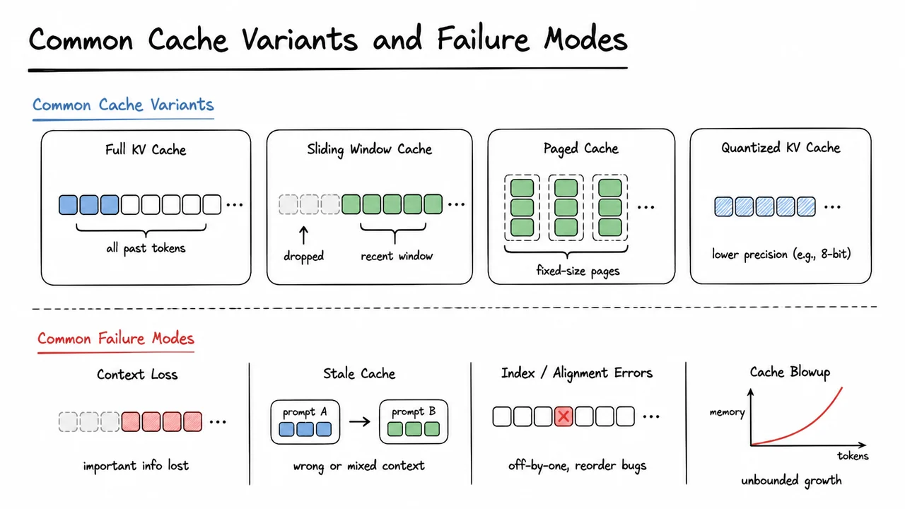
But once you move from “toy correctness” to production decoding, the cache stops being a single obvious object. One common variant is a prefill + decode split: the prompt is processed in a batched prefill phase that fills the cache for the entire context, and then generation proceeds token by token using only incremental updates. Another variant is paged or block-based caching, where memory is managed in fixed-size chunks so that variable-length sequences can grow without costly contiguous reallocation. There are also systems that use sliding-window caches, keeping only the most recent tokens to bound memory, which is an approximation rather than an exact implementation of full-context attention.
These variants exist because the cache creates a sharp compute–memory tradeoff. Caching removes redundant attention work, but it also stores tensors whose size grows with context length, number of layers, heads, and head dimension. Roughly speaking, for layers, heads, head dimension , and context length , the cache footprint scales like That scaling is why long-context decoding becomes memory-bound long before it becomes mathematically difficult. In other words, caching makes generation faster by avoiding recomputation, but it does so by spending the very resource—device memory—that is often most constrained at inference time.
The key practical insight is that a cache is only useful if its assumptions match the decoding regime. Autoregressive decoding assumes the prefix is fixed. If the prefix changes, the cache is stale. This happens more often than beginners expect:
- Prompt editing or truncation: removing or inserting tokens invalidates later cached states.
- Batching with heterogeneous sequence lengths: each sequence needs its own valid cache region.
- Speculative or branchy decoding: a rejected draft path must not leak into the committed cache.
- Sliding-window attention: older cache entries may be intentionally dropped, but then the model’s behavior changes by design.
A related failure mode is shape or layout mismatch. Many inference kernels assume a specific memory layout for the cache, such as contiguous head-major or block-packed storage. If the implementation silently permutes dimensions, reuses buffers incorrectly, or confuses layer order with token order, the model may still run while producing numerically plausible but wrong outputs. These bugs are especially dangerous because they do not always crash; they just degrade generation quality in a way that looks like “the model got worse.”
There is also a semantic failure mode: some cache variants are exact, while others are approximations. A full cache preserves the exact attention distribution of naive decoding, but a truncated or compressed cache does not. That difference matters when evaluating systems. A faster cache that changes the model’s output distribution is not merely an optimization; it is a different inference algorithm. Production systems often accept this tradeoff only when the lost context is unlikely to matter, or when latency constraints dominate exactness.
The visual below condenses these ideas into a small set of contrasting cache variants and the failure modes they invite. The goal is not to memorize every implementation detail, but to internalize the organizing principle: every cache design is a promise about reuse, and every failure mode is a violation of that promise. Once you see the variants side by side, it becomes easier to reason about why a system chooses one layout over another, and why seemingly minor changes—like truncation, block sizing, or reordering—can have outsized effects on correctness and speed.
15. KV Caching: Equivalent Views and Practical Takeaways
Once we move from “why caching is exact” to “how we actually deploy it,” the right mental model is no longer a single implementation trick but a family of equivalent views of the same computation. That matters because KV caching is often described differently in code, papers, and production systems, yet these descriptions are all trying to preserve one invariant: under causal attention, the token at time only needs the keys and values from positions , never from the future.
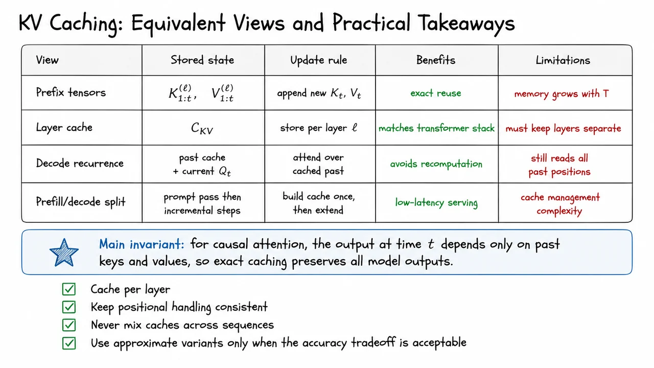
The simplest view is to treat each layer’s cache as a growing prefix tensor. For layer , when a new token arrives, we append its key and value: This formulation is almost embarrassingly direct, which is precisely why it is useful. It makes the exactness argument transparent: if the attention for position is causal, then recomputing old prefixes is pointless, because the new output only depends on the new query and the cached past . The catch is that the cache grows with sequence length , so the memory footprint can become the bottleneck long before arithmetic does.
A second view is the layer cache perspective: This emphasizes that a transformer is not one monolithic attention block but a stack of layers, each with its own hidden-state history. That distinction is not cosmetic. Keys and values from different layers live in different representation spaces, so they must be stored separately and indexed consistently with the layer that produced them. A common failure mode in implementation is to treat the cache as if it were a generic buffer, when in fact layer identity is part of the state.
A third equivalent view is the decode recurrence: at time , compute the current query , fetch the past cache, and form attention against cached history rather than reprocessing the entire prefix. Algebraically, this changes the organization of computation, not the function being computed. The model still performs the same softmax over the same eligible keys and values; it simply avoids repeating the projection work for earlier tokens. In practical terms, this is the reason autoregressive serving can be fast enough to feel interactive instead of quadratic in the length of the generated continuation.
The final operational view is the prefill/decode split. During prefill, the prompt is processed once to build the cache; during decode, each new token extends that cache incrementally. This split is the basis of low-latency inference systems because it separates the expensive one-time prefix computation from the much cheaper token-by-token loop. But it also introduces systems complexity: cache allocation, sequence bookkeeping, eviction policies, and batching all become part of the correctness story, not just the performance story.
What unifies these views is the exactness invariant. If attention is causal, then all of these formulations preserve the model’s outputs because they reuse only the information that the full forward pass would have used anyway. The reason this works is subtle but fundamental: attention is a function of the query at the current position and the historical key-value pairs, so caching is not an approximation to the model; it is a memoization of its past internal state. Where this breaks down is equally important:
- if positional handling changes between prefill and decode, the cache no longer aligns with the model’s notion of order;
- if caches from different sequences are mixed, the model may attend to чужой history and produce garbage;
- if one uses compressed, quantized, or truncated variants, the output may remain useful but is no longer guaranteed exact.
That is why production systems treat KV caching as both an algorithmic optimization and a state-management problem. The main tradeoff is simple to state but hard to engineer around: time goes down, memory goes up. The more aggressively you optimize decode latency, the more carefully you must manage cache layout, lifetime, and isolation across requests.
The visual below condenses these equivalent formulations into one compact summary. A table is especially effective here because the point is not that the views are different, but that they are the same computation seen through different engineering lenses: what is stored, how it is updated, what benefit it provides, and what limitation remains. The invariant callout reinforces the real reason caching is exact, while the checklist reminds you of the deployment rules that keep the mathematics intact in practice.