LoRA Fine-Tuning: Low-Rank Adaptation of Large Neural Networks
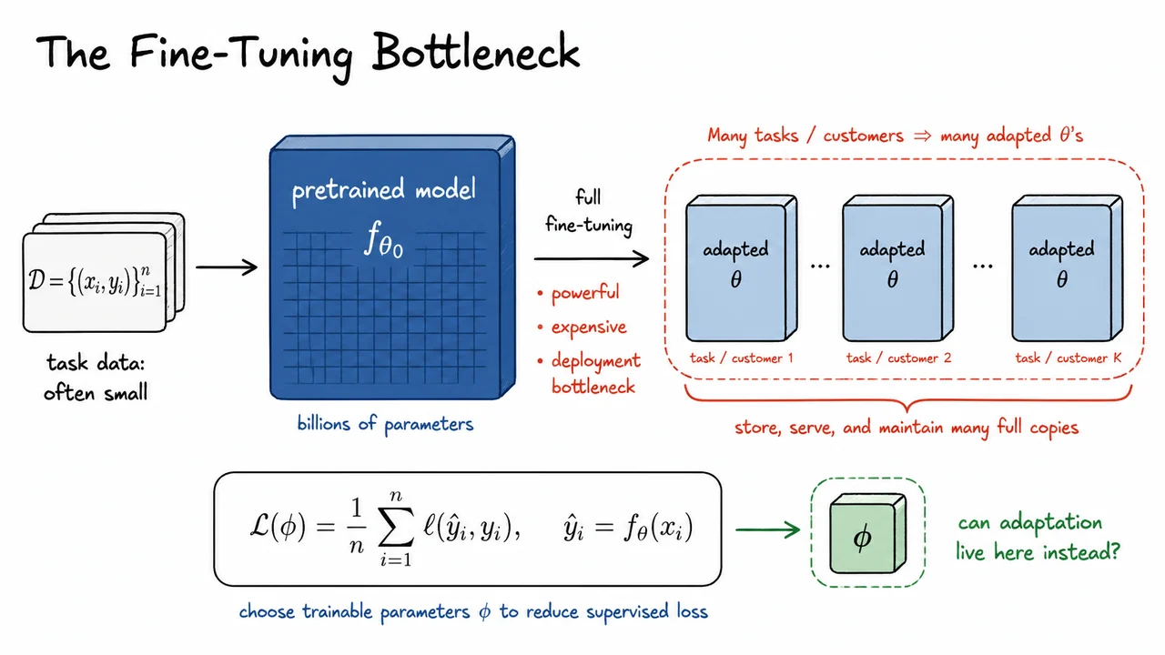
Before we get to LoRA itself, it is worth slowing down on the pressure point that made methods like LoRA necessary. Modern pretrained models are powerful precisely because they concentrate enormous general-purpose knowledge into a parameter vector . But that same scale turns the most obvious adaptation strategy—just fine-tune everything—into a systems problem as much as a learning problem.
Suppose we start with a pretrained model and a supervised downstream dataset
For a task such as sentiment classification, medical extraction, instruction following, or customer-specific generation, adaptation means changing something about the model so that its predictions better match the desired outputs . Abstractly, we choose some trainable parameters and minimize the empirical loss
The important detail is that does not have to be the entire model. It simply denotes whatever parameters we decide are allowed to move during adaptation. In full fine-tuning, we make the maximal choice: initialize , set , and optimize every parameter of the pretrained model.
This is a very strong baseline. Full fine-tuning gives the optimizer direct access to every layer, every attention projection, every MLP weight, every embedding table, and every normalization parameter. If the downstream task needs a subtle redistribution of features throughout the network, full fine-tuning can in principle make those changes. That flexibility is one reason it often performs well when we have enough data, compute, and careful regularization.
The bottleneck is that flexibility is expensive. A model with billions of parameters is not just expensive to pretrain; it is expensive to repeatedly copy, optimize, store, serve, version, and audit. During training, full fine-tuning typically requires optimizer state for every trainable parameter. With Adam-like optimizers, that can mean storing the parameter, its gradient, and multiple moment estimates. The memory footprint can become several times larger than the model weights alone.
The deployment cost is even more direct. If we fine-tune a separate full model for each task or customer, then each adaptation produces another full-sized parameter vector:
Even if each differs only slightly from the original , naive full fine-tuning stores every adapted copy independently. For a 7B, 13B, or 70B parameter model, this quickly becomes impractical. The problem is not merely training one model once; the problem is supporting many adapted models.
There is also a statistical subtlety. Downstream datasets are often much smaller than the pretraining corpus. When is small and has billions of trainable degrees of freedom, the model has enough capacity to memorize idiosyncrasies of the task dataset. Good fine-tuning practice therefore relies on learning-rate schedules, regularization, early stopping, validation sets, and sometimes freezing parts of the network. Full fine-tuning is powerful, but it is not automatically data-efficient or operationally convenient.
This motivates the central question behind parameter-efficient fine-tuning:
> Can we keep the pretrained weights frozen, while letting a much smaller set of parameters carry the task-specific adaptation?
If the answer is yes, then we can reuse one large shared model and store only a small task-specific delta for each downstream use case. Instead of maintaining many full copies of , we maintain one base model plus many compact adaptations. LoRA will instantiate this idea by restricting the update to certain weight matrices and forcing that update to have low rank, but the motivation starts here: most of the pretrained model should remain a reusable shared asset.
A useful way to frame the trade-off is:
The visual below compresses this argument into a left-to-right bottleneck: a small task dataset feeds into a huge pretrained model, full fine-tuning produces separate large adapted models, and the cost grows with the number of tasks or customers. The key asymmetry is that the task data and desired behavioral change may be small, while the object being duplicated is enormous.
The small placeholder in the diagram points toward the idea LoRA will develop next. Instead of asking every parameter in to move, we will ask whether adaptation can live in a much lower-dimensional space—small enough to store and train cheaply, but expressive enough to recover much of the performance of full fine-tuning.
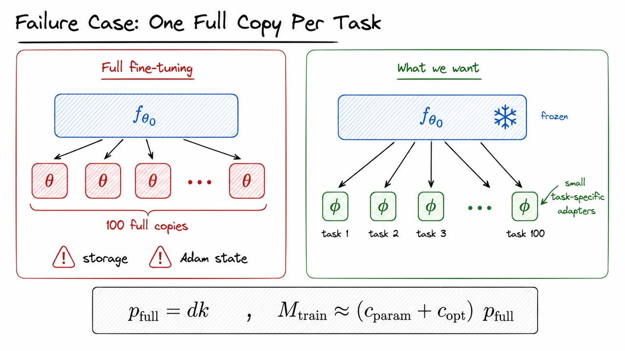
The optimization view from the previous section makes full fine-tuning look deceptively simple: start from a pretrained parameter vector , optimize the downstream loss, and obtain an adapted parameter vector . Conceptually, that is clean. Operationally, however, it hides the main scaling problem: after fine-tuning, is no longer a universal shared object. It is now task-specific.
If we adapt the same pretrained model to one downstream task, this may be acceptable. But the whole point of large pretrained models is that they are reused across many tasks: summarization, code generation, retrieval-augmented QA, domain-specific chat, instruction following, classification, extraction, and so on. With full fine-tuning, adapting one base model to 100 downstream tasks gives 100 distinct full model checkpoints. Each checkpoint contains a complete copy of the model parameters, even if the actual task-specific change from is small.
For a single dense weight matrix , full fine-tuning treats every entry as trainable. The number of trainable parameters in that matrix is therefore
This looks harmless at the matrix level, but modern transformers contain many such matrices: attention projections, MLP projections, embeddings, output heads, and normalization-related parameters. Full fine-tuning scales with the size of the entire model, not with the amount of information needed to specialize the model to the task.
The training memory cost is even worse than the checkpoint size suggests. During training, we do not only store the parameters themselves. We also store gradients, activations needed for backpropagation, and optimizer state. For Adam-like optimizers, each trainable parameter typically carries additional moment estimates, often the first and second moments. Abstracting away implementation details, the memory footprint associated with trainable parameters can be summarized as
where accounts for storing trainable weights and related parameter-level quantities, while accounts for optimizer state. The important point is not the exact constant; it is the scaling. If every parameter is trainable, Adam allocates optimizer state for every parameter.
This creates a practical failure mode that is easy to underestimate. The base model may be shared in theory, but full fine-tuning destroys that sharing in deployment. Each task now needs its own full checkpoint. Serving many variants requires model routing, checkpoint loading, memory residency decisions, version management, and duplicated storage. If the base model has billions of parameters, even “just one more fine-tuned task” can become expensive.
The key inefficiency is that full fine-tuning assumes the task-specific solution must be represented as an entirely new point in the full parameter space. But empirically, many downstream adaptations appear to require only a comparatively small change in behavior. We would like to capture that change without rewriting and storing the entire model. In other words, the desired pattern is:
This is the motivation behind parameter-efficient fine-tuning. Rather than asking, “How do we find a new full model for each task?”, we ask, “Can we represent the task-specific update compactly?” LoRA will answer this by constraining updates to certain weight matrices to have low rank, but before getting there, it is important to see the failure case clearly: full fine-tuning pays the full model cost even when the useful adaptation may be much smaller.
The visual below compresses this contrast into two patterns. On the left is the full fine-tuning regime: one shared pretrained model gives rise to many separate full checkpoints, with storage and Adam state growing with the full parameter count. On the right is the parameter-efficient goal: keep frozen and shared, while attaching small task-specific parameters .
The equation at the bottom anchors the intuition mathematically. For a fully trainable matrix, , and the training footprint scales like . The rest of the lecture is about replacing that scaling law with something much smaller, while preserving most of the quality benefits of fine-tuning.
The “one full copy per task” failure mode suggests a natural repair: stop treating every downstream task as a reason to duplicate the whole model. If the pretrained parameters already encode broadly useful linguistic, visual, or multimodal structure, then perhaps task adaptation should be a small correction rather than a complete rewrite. This is the core motivation behind parameter-efficient fine-tuning: keep the base model frozen, and learn only a comparatively tiny set of task-specific parameters .
In abstract form, most PEFT methods follow the same pattern:
This changes the economics of fine-tuning. Instead of storing and serving a separate full model for each task, we store one shared pretrained backbone plus many small task modules. Training also becomes cheaper because gradients, optimizer states, and parameter updates are needed only for , not for the full . For very large models, this distinction is not cosmetic: optimizer states alone can multiply memory requirements several times over the raw parameter count.
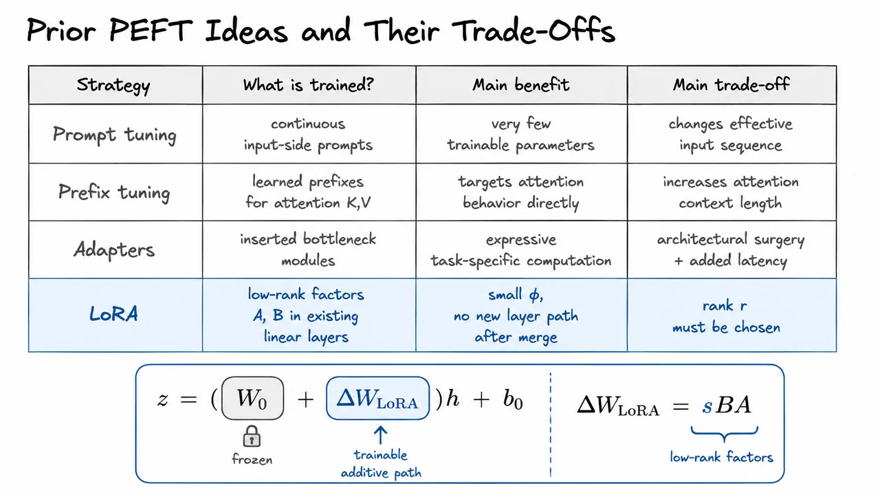
But “freeze the model and train something small” is not a complete algorithm. The hard question is where to put the small trainable object so that it has enough influence over the computation. Different PEFT methods answer this question differently, and their trade-offs are mostly about the location and form of .
Prompt tuning puts the trainable parameters at the input side. Instead of updating the transformer weights, we prepend learned continuous prompt vectors to the input embeddings. This can be extremely parameter-efficient because the trainable object is just a small collection of vectors. However, it also means the model is adapted indirectly: the only way the task signal can affect the network is by changing the effective input sequence. That can be elegant, but it may be too weak for tasks requiring deeper internal changes, and it consumes part of the model’s context budget.
Prefix tuning is more targeted. Rather than adding learned vectors only at the input embedding layer, it learns prefix states that are injected into attention, often as additional key/value vectors. This gives the task parameters a more direct handle on attention patterns: the model can attend to learned task-specific memory at each layer. The cost is that these prefixes increase the effective attention context length, which can add computation and memory overhead during inference. The base weights remain frozen, but the runtime attention path is now larger.
Adapters take a different route: they insert small neural modules inside the network, commonly bottleneck MLPs placed between or within transformer sublayers. A typical adapter maps a hidden state down to a low-dimensional space, applies a nonlinearity, maps it back up, and adds the result residually. This is more expressive than input-side prompt methods because it creates new task-specific computation throughout the model. The downside is architectural surgery. The model’s forward graph now contains extra modules, which can introduce latency and complicate deployment, especially when we care about highly optimized inference kernels.
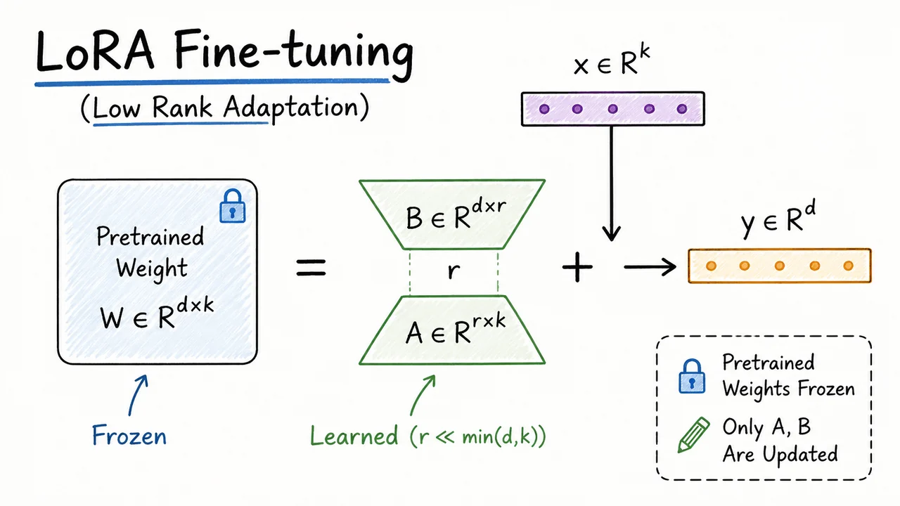
LoRA belongs to this PEFT family, but its design choice is more surgical: instead of changing the input sequence, extending attention context, or inserting new nonlinear modules, it modifies the effective weights of existing linear layers. The pretrained weight is frozen, but the layer behaves as though it had received an additive update:
The crucial constraint is that this update is not a full dense matrix. LoRA parameterizes it as a low-rank product:
where and are trainable low-rank factors and is a scaling factor. If , then a full update would require trainable parameters. LoRA instead uses something like
for a total of
trainable parameters. When , this is dramatically smaller than a dense update.
This design gives LoRA an important deployment advantage over many earlier PEFT methods: after training, the learned update can often be merged into the frozen weight by replacing with . At inference time, the layer can remain an ordinary linear transformation. There is no extra prompt length, no additional attention prefix, and no new adapter branch that must be executed separately. The trade-off is that LoRA’s expressiveness is controlled by the rank . If is too small, the update may be unable to represent the adaptation the task needs; if is too large, we lose some of the parameter-efficiency and memory benefits.
So the PEFT landscape can be summarized by a simple comparison:
The visual below consolidates this comparison. The first three methods all preserve the frozen pretrained backbone, but they attach task-specific capacity in different places: before the model, inside attention state, or as inserted modules. LoRA is highlighted because it keeps the computation closest to the original linear layer while still allowing a learned task-specific correction.
The equations underneath the comparison are the key transition into the next idea. LoRA is not merely “another small module”; it is a hypothesis about the geometry of fine-tuning itself: perhaps the useful update does not need to occupy the full matrix space. If task adaptation lives in a low-dimensional subspace, then the factorization is not just a memory trick — it is a structured constraint on how the pretrained model is allowed to move.
The tension with earlier PEFT methods is that they save parameters by adding something around the pretrained model: prompts, adapters, extra bottlenecks, or task-specific modules. That can work well, but it raises an important question: do we really need to alter the architecture or insert new computation paths, or can we express task adaptation as a small change to the weights that are already there?
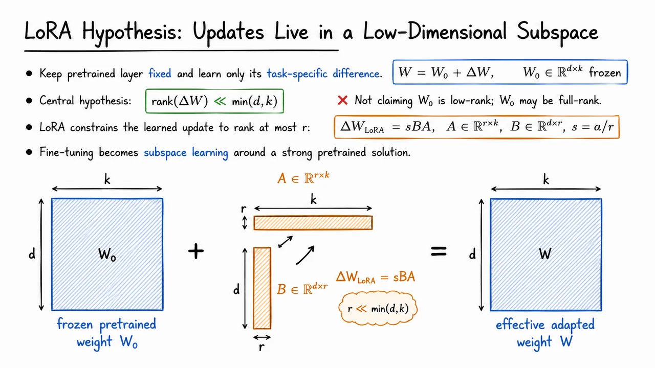
LoRA starts from a very direct view of fine-tuning. Suppose a pretrained linear layer has weight matrix . In ordinary full fine-tuning, we replace it with a new learned matrix . Equivalently, we can write the final weight as the pretrained matrix plus a task-specific displacement:
This decomposition is conceptually useful because it separates two roles. The pretrained matrix already contains broad linguistic, visual, or multimodal structure learned from large-scale pretraining. The downstream task does not usually require relearning all of that structure from scratch. Instead, it may only need to steer the pretrained transformation in a relatively small number of directions.
The central LoRA hypothesis is therefore not that the pretrained weight itself is simple. may be full-rank, dense, and highly expressive. The claim is about the update induced by downstream fine-tuning:
In words: although has the same shape as , the meaningful change needed for a task may lie in a much lower-dimensional subspace. This is plausible in large pretrained models because many downstream tasks are not asking the model to invent entirely new representations; they are asking it to recombine, emphasize, suppress, or redirect features that already exist.
A useful geometric picture is to think of full fine-tuning as allowing movement in every direction in the -dimensional weight space. LoRA assumes that the useful displacement from lives near a much smaller manifold or subspace. Rather than learning every entry of independently, we restrict to have low rank by factorizing it:
Here is the LoRA rank, usually chosen much smaller than or . The matrix projects the input into an -dimensional adaptation space, and maps that low-dimensional signal back into the output dimension. The scalar controls the scale of the update, making the adaptation strength easier to tune across different ranks.
This factorization immediately gives the rank constraint. Since is the product of a matrix and an matrix,
So LoRA does not merely hope that the update will be low-rank; it enforces that constraint by construction. The learned update cannot use more than independent directions, no matter how large the original matrix is.
The parameter savings follow from the same structure. A full update would require trainable parameters. LoRA learns only and , requiring
parameters. When , this is dramatically smaller than . For example, if and , a full update has over 16 million parameters, while the LoRA update has only parameters for that layer.
The subtle but important point is that LoRA turns fine-tuning into subspace learning around a strong pretrained solution. We are not training a small model instead of a large one. We are using the large model as a fixed base and learning a compact task-specific displacement. This is why LoRA can often preserve the capabilities of the pretrained model while adapting efficiently: the expressive burden remains mostly in , and the trainable part only needs to encode the difference.
There are also failure modes hidden inside the hypothesis. If a task genuinely requires many independent changes to a layer, a very small rank may underfit. If the inserted LoRA modules are placed in layers or projections that are not important for the task, the low-rank update may be parameter-efficient but ineffective. And if the downstream distribution is far from pretraining, the assumption that adaptation is a small low-dimensional displacement may become weaker. LoRA is powerful precisely when the pretrained representation is already close and the task mostly needs targeted steering.
The visual below can be read as a compact summary of this idea. The large frozen matrix represents the stable pretrained transformation. The small low-rank branch, formed by and , represents the lightweight trainable update . The adapted weight is not a completely new matrix learned from scratch; it is the frozen base plus this constrained task-specific correction.
The key contrast is visual as much as mathematical: remains large and expressive, while the learned update is deliberately narrow. The annotation captures the LoRA bet: most of the useful downstream movement can be expressed through a small number of adaptation directions.
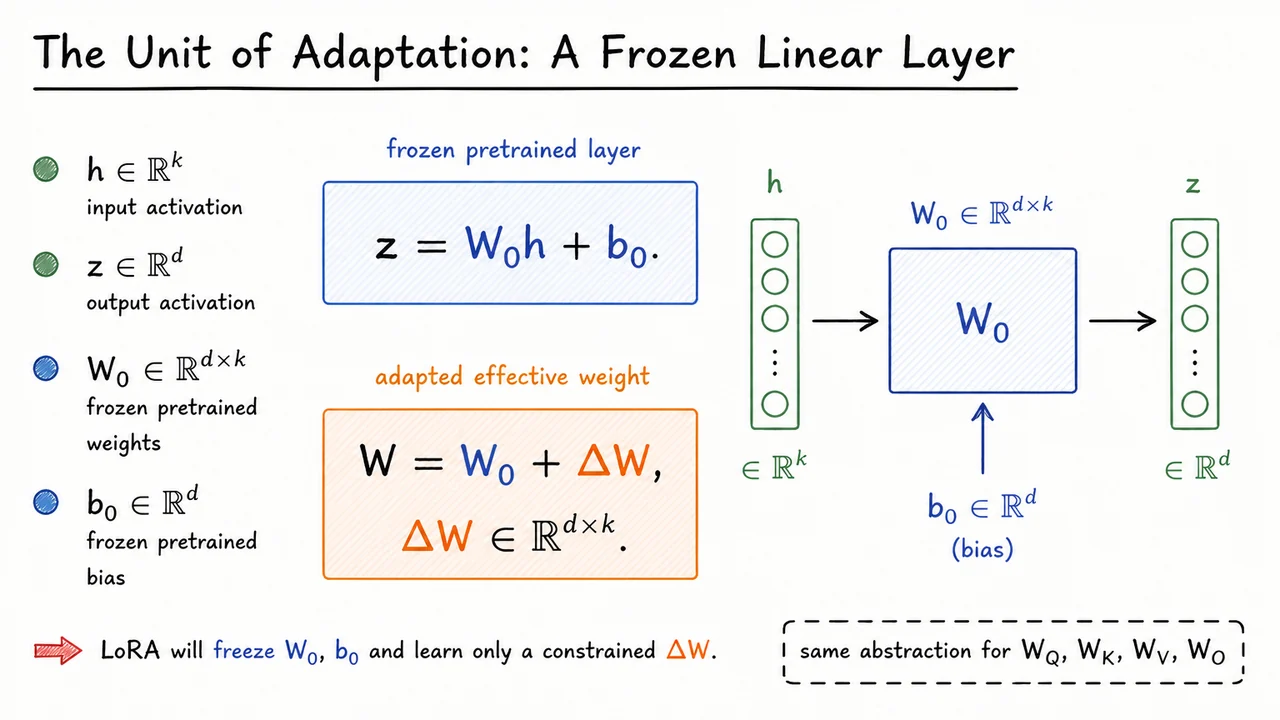
Having argued that task-specific changes may live in a much smaller subspace than the full parameter space, we now zoom in to the smallest object where LoRA actually acts: one linear layer. This is the right level of abstraction because transformer blocks are built from many affine maps—query, key, value, output projections, MLP projections—and fine-tuning ultimately changes the matrices inside those maps.
Consider a pretrained linear layer receiving an activation vector and producing an output vector . Before any adaptation, the layer computes
where is the pretrained weight matrix and is the pretrained bias. The subscript is important: it reminds us that these parameters come from pretraining and are treated as the reference point around which adaptation happens.
Full fine-tuning would simply allow and to move freely during task training. But LoRA begins from a different framing. Instead of saying “we learn a new weight matrix,” we say: the adapted model uses an effective weight
Here, is the task-specific correction to the pretrained matrix. If , we recover the original model exactly. If is unrestricted, this is just another way of writing ordinary weight fine-tuning. The key move in LoRA will be to keep fixed and learn only a structured version of .
This additive view is more than notation. It separates two roles that are entangled in full fine-tuning:
That distinction is what makes parameter-efficient fine-tuning possible. We do not need to rewrite the pretrained model from scratch; we need to learn a correction that steers its existing computation toward a new task or distribution.
There is also a subtle but useful assumption here: LoRA treats adaptation as a perturbation around a strong pretrained solution. That assumption is usually reasonable when the downstream task is related to the model’s pretraining distribution, but it can fail when the new task demands behavior far outside the pretrained model’s capabilities. In such cases, a small or low-rank may not have enough expressive power, and full fine-tuning—or a larger adaptation mechanism—may be necessary.
At this point, is still a full matrix. So we have not yet saved parameters. We have only changed our perspective from “learn the whole weight” to “learn an update to a frozen weight.” The next step will be to constrain to have low rank, but the additive decomposition itself is the core abstraction:
In LoRA, and typically remain frozen during training. Gradients flow through the layer as usual, but only the parameters used to construct are updated. This preserves the pretrained matrix exactly, reduces optimizer state, and allows multiple task-specific adaptations to be stored separately while sharing the same base model.
The same abstraction applies directly to transformer projection matrices such as , , , and . Each is just a linear map from one activation space to another. LoRA does not require a special transformer-specific derivation at this stage; it only requires identifying which linear maps should receive learned additive updates.
The visual below condenses this idea into one frozen affine layer and its adapted counterpart. The blue components represent the pretrained computation , while the orange update marks the only part that will later become trainable under LoRA’s low-rank parameterization.
Read it as a bridge between standard fine-tuning and LoRA: first define the effective adapted weight ; then, in the next step, restrict the shape of so that adaptation becomes dramatically cheaper without discarding the pretrained layer.
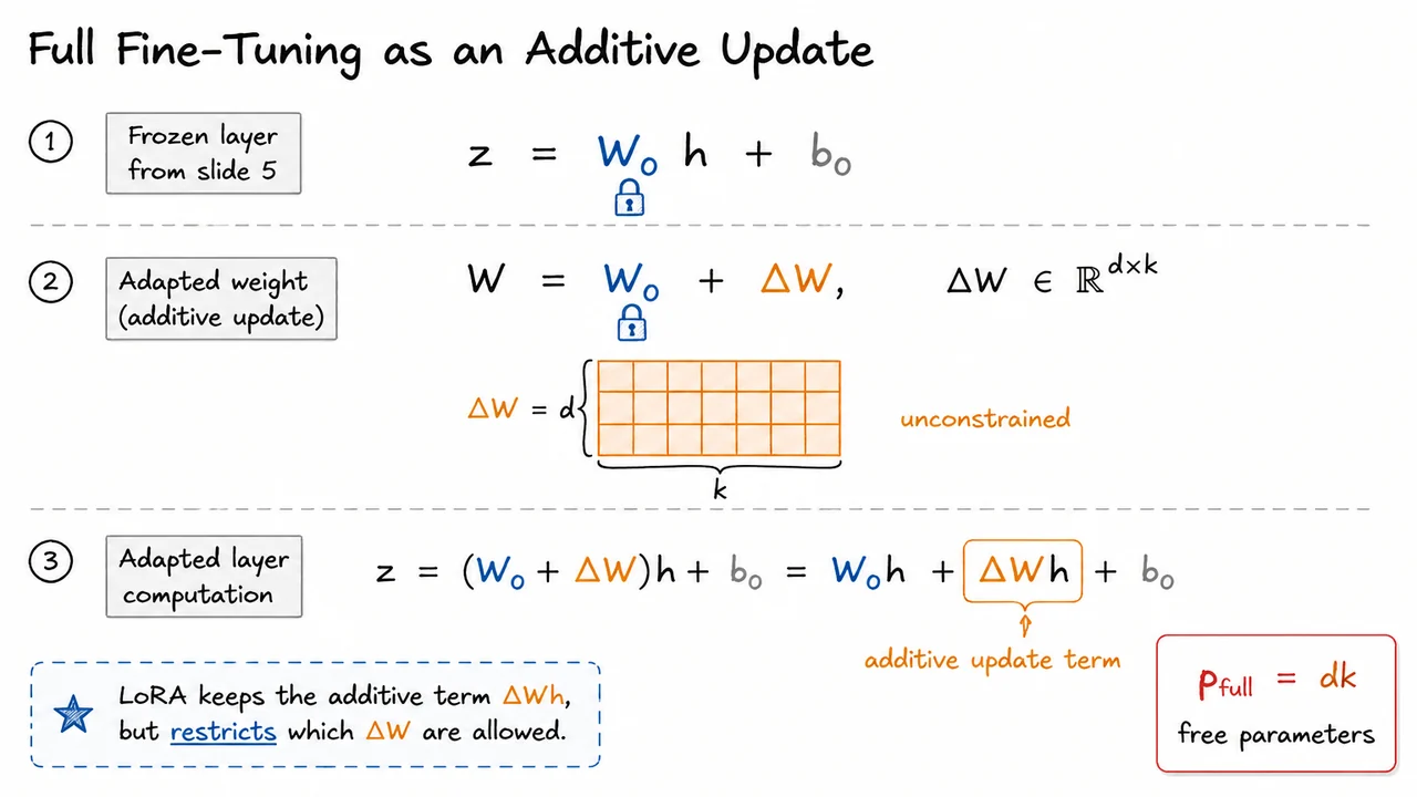
Now that we have isolated a single frozen linear layer, the next step is to ask what full fine-tuning actually changes at that layer. The usual description says that fine-tuning “updates the weights,” but for LoRA the more useful viewpoint is slightly different: full fine-tuning learns an additive correction to the pretrained matrix.
Start from the frozen layer
where , , and . The matrix is the pretrained weight we inherited from the base model. During full fine-tuning, we replace it by a new adapted matrix . But any such adapted matrix can always be written as
This is not yet an approximation or a LoRA assumption. It is just algebra. Given any final fine-tuned weight , the difference
is the update that full fine-tuning has learned relative to the pretrained model.
Substituting this decomposition back into the layer gives
By distributing over , we get
This expression is the key abstraction. The adapted layer can be understood as the original pretrained computation , plus an additional task-specific correction . In other words, fine-tuning does not need to be viewed as replacing the pretrained model wholesale. At the level of one linear layer, it is equivalent to keeping the pretrained transformation and adding a learned residual transformation.
Under full fine-tuning, however, the update is completely unconstrained. Since has the same shape as , it contains
free parameters for this layer alone. Every entry of the matrix may move independently. If the layer maps a -dimensional activation into a -dimensional output, full fine-tuning allows an arbitrary linear correction from to .
That flexibility is powerful, but it is also expensive. In modern transformers, the major weight matrices are large, and there are many of them. Updating all of their entries means we must:
The subtle point is that LoRA does not begin by removing the additive correction . It keeps exactly this residual-update interpretation. What LoRA changes is the space of matrices that is allowed to occupy. Full fine-tuning says: “learn any matrix .” LoRA will say: “learn a structured, low-rank matrix that is much cheaper to represent.”
This distinction matters because it explains why LoRA can be inserted into an existing pretrained model without changing the basic forward computation. The layer still produces the frozen pretrained contribution , and it still adds an adaptation term. The efficiency gain comes from parameterizing that adaptation term more carefully, not from inventing a new kind of layer.
The visual below compresses this logic into three pieces: the original frozen layer, the decomposition , and the adapted computation where the correction appears explicitly as . The color separation is important: pretrained quantities remain frozen, while the update matrix is the trainable object.
It also highlights the cost of doing this without constraints. The orange block represents an unconstrained update matrix with free parameters. This is the baseline LoRA will improve upon: not by denying that full fine-tuning learns an additive update, but by restricting that update to a much smaller low-rank family.
Having written full fine-tuning as a frozen pretrained map plus an additive correction, the natural next question is: how expressive does that correction really need to be? If a layer originally computes
then full fine-tuning replaces by , so the adapted layer becomes
The key observation is that, for this layer, all task-specific adaptation enters through the vector . We do not directly care about as an abstract matrix; we care about the directions in activation space that it can add to the frozen pretrained computation.
A completely unrestricted can represent any linear correction from the input activation space to the output activation space . Geometrically, this means the update may use as many as independent output directions. That is powerful, but expensive: it requires learning new degrees of freedom for a single weight matrix. In large transformers, many such matrices are enormous, so repeating this across attention and MLP layers quickly becomes the dominant storage and optimization cost.
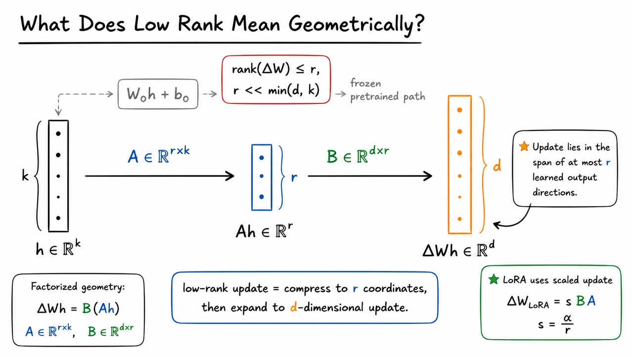
LoRA’s central bet is that useful downstream adaptation often lives in a much smaller subspace. Instead of allowing to be arbitrary, we constrain it to have low rank:
This is not merely a parameter-count trick. It is a geometric restriction on what kinds of changes the model can make. A rank- matrix can only map inputs into an output subspace of dimension at most . So although is still a vector in , as varies it can only move within at most learned directions inside that -dimensional output space.
The most useful way to see this is through factorization. Any rank-at-most- update can be represented as the product of two thinner matrices:
where
Then the update applied to an activation becomes
This equation is the geometric heart of LoRA. The matrix first compresses the original -dimensional activation into coordinates:
Then expands those coordinates back into a -dimensional update vector:
So the update is forced through an -dimensional bottleneck. The model can still produce a full-sized correction vector, but that correction must be assembled from at most learned basis directions: the columns of . The compressed vector supplies the coefficients for combining those directions.
This also clarifies both the strength and the limitation of LoRA. If the task-specific change really is concentrated in a low-dimensional subspace, then a small can capture it efficiently. But if adaptation requires many independent directions — for example, if the downstream task demands a broad reorganization of the layer’s representation — then too small a rank may underfit. In that case, the bottleneck is not just saving parameters; it is actively preventing certain updates from being represented.
LoRA usually adds one more scaling factor:
The scalar controls the magnitude of the low-rank branch relative to the frozen pretrained path. This matters because the matrices and are trained from initialization, while already contains a large amount of pretrained structure. The scaling helps make the injected update numerically stable and comparable across different choices of rank .
A compact way to remember the whole construction is:
The visual below consolidates this idea as a flow: the input activation is first passed through , producing a narrow -dimensional bottleneck , and then through , producing the full output update . The frozen pretrained computation remains in the background, while the colored low-rank branch shows exactly where adaptation is being inserted.
The important thing to notice is not just that the middle vector is smaller. The bottleneck is what enforces the rank constraint. Since every update must pass through coordinates before being expanded, the final correction can only span an -dimensional family of output movements. That is the geometric meaning of “low rank” in LoRA: compress to a small learned coordinate system, then expand into a controlled task-specific update.
The geometric picture of low rank gives us the right intuition: a low-rank matrix can only move inputs through a small-dimensional subspace before expanding them back out. LoRA turns that intuition into a concrete parameterization for fine-tuning. Instead of learning an arbitrary dense update , we force the update to pass through an -dimensional bottleneck.
For a pretrained weight matrix , full fine-tuning would replace it by
where has the same shape as and contains trainable parameters. LoRA keeps frozen and constrains the trainable update to have the factorized form
Here
The multiplication order is important. An input vector in is first projected down by into , then projected back up by into . The scalar controls the magnitude of the LoRA update; it does not change the rank or the number of trainable parameters. It is best understood as a scaling convention that helps make different choices of comparable during optimization.
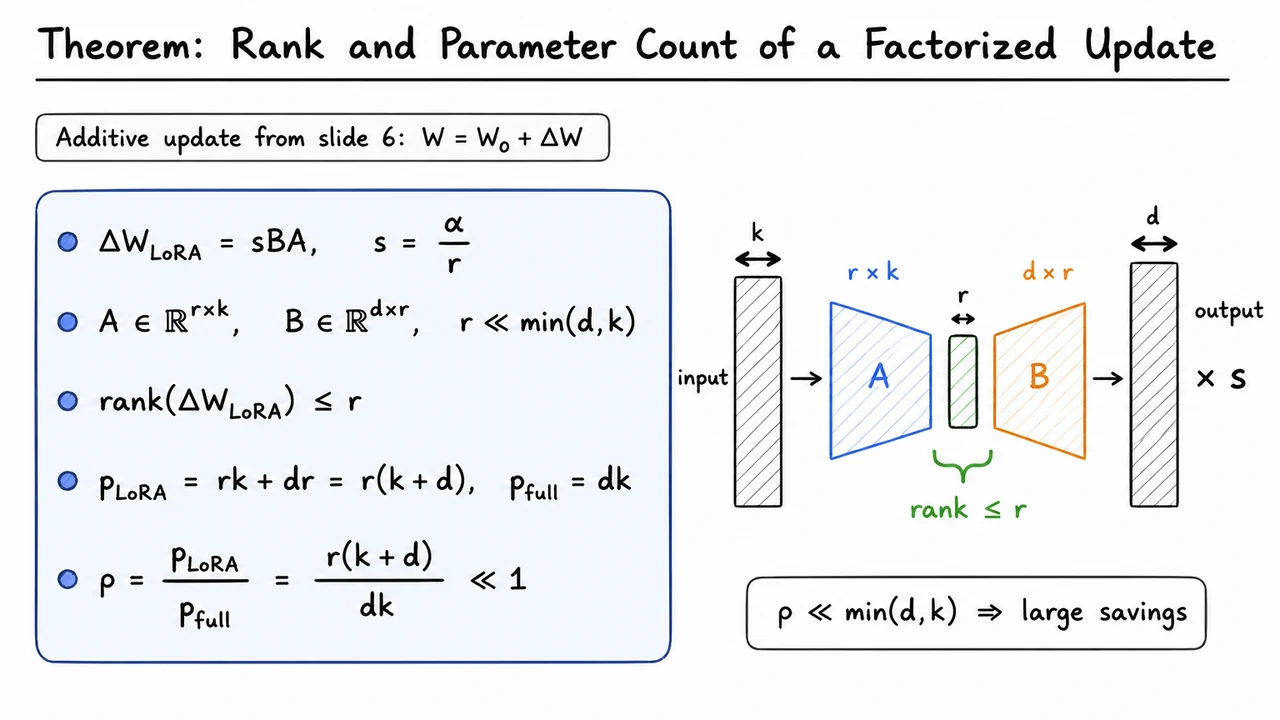
The key theorem is simple but powerful:
This is the formal version of the bottleneck story. No matter how large and are, the product cannot have rank larger than the intermediate dimension . The update may live inside a huge matrix, but its degrees of freedom are constrained to flow through an -dimensional channel.
That constraint is exactly what makes LoRA parameter-efficient. Instead of training all entries of , we train only the entries of and :
By contrast, a full update would require
So the trainable-parameter fraction is
When , this ratio can be very small. For example, if and , then full fine-tuning uses over 16 million trainable parameters for that matrix, while LoRA uses only . That is about of the full parameter count for the layer.
There is a subtle but important distinction here: LoRA is not saying the weight matrix itself is low rank. The pretrained matrix remains full-size and may be full-rank. LoRA only constrains the change applied during adaptation:
This matters because the model can still use the rich representation already stored in . LoRA merely assumes that the task-specific correction needed for fine-tuning lies in a much smaller subspace than the original model weights.
This assumption can fail. If a new task requires many independent directions of change in a layer, then a very small may underfit. Increasing gives the update more expressive capacity, but also increases memory, optimizer state, and potential overfitting. The practical appeal of LoRA comes from the empirical observation that many adaptation tasks do not require a full-rank update everywhere; a modest bottleneck often captures most of the useful task-specific movement.
The visual below compresses the theorem into one picture: an unconstrained dense update is replaced by two thinner matrices, and , with a narrow -dimensional passage between them. The green bottleneck is the reason for the rank bound, while the separate parameter counts remind us why the method is attractive computationally.
It is useful to read the diagram from left to right as a computation and from top to bottom as a theorem. Computationally, inputs pass through , then , then the scalar . Mathematically, the same factorization guarantees and reduces the number of trainable parameters from to .
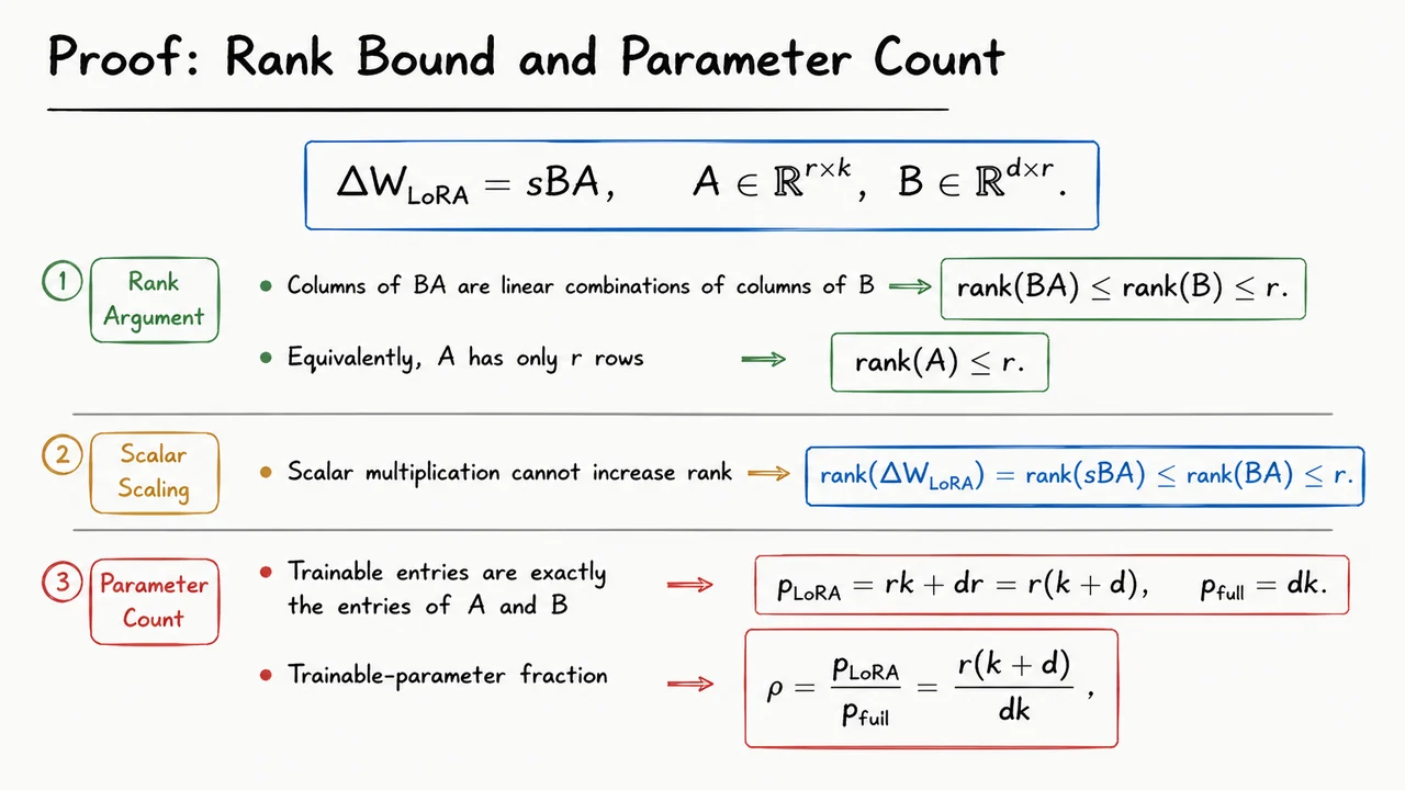
The theorem gives us the punchline; now we should make the proof feel almost inevitable. LoRA’s efficiency is not a mysterious property of transformers or attention layers. It comes from a simple linear-algebra fact: if we force an update matrix to factor through a small -dimensional bottleneck, then the update cannot have rank larger than , and the number of trainable parameters is the size of the two skinny factors rather than the size of the full matrix.
Suppose a pretrained layer contains a frozen weight matrix . Full fine-tuning would learn an arbitrary update , so the adapted weight would be
LoRA restricts the update to the factorized form
Here is the LoRA rank, usually chosen much smaller than both and , and is a scalar scaling factor. The important structural point is that the update does not map directly from to with a fully flexible matrix. Instead, it first passes through an -dimensional intermediate space via , and then maps back up to dimensions via .
That bottleneck immediately limits the rank. One way to see this is column-wise. The product has columns, and each column is obtained by multiplying by the corresponding column of . Therefore every column of lies in the column space of . Since has only columns, its column space has dimension at most . Thus
Equivalently, we could reason from the other side: has only rows, so , and the rank of a product cannot exceed the rank of either factor. Both perspectives say the same thing: the factorization forces the update to move within a low-dimensional subspace of possible full updates.
The scalar does not change this conclusion. If , multiplying by rescales every singular value but does not create new nonzero singular values. If , the update becomes the zero matrix, whose rank is even smaller. So in all cases,
This is the rank-bound half of the proof: LoRA is not merely encouraging a low-rank update; it parameterizes the update so that low rank is guaranteed.
The parameter-count argument is just as direct. In full fine-tuning, the update has one trainable parameter for every entry of a matrix:
In LoRA, the original matrix is frozen. The only trainable entries are those in and . Matrix contributes parameters, and matrix contributes parameters, so
The trainable-parameter fraction is therefore
When , this fraction can be tiny. For square matrices with , it becomes approximately
so the savings grow as the layer width grows. This is precisely why LoRA becomes more attractive for large models: the full matrix scales quadratically in width, while the factorized update scales linearly in width for fixed .
There is a subtle but important trade-off hiding inside this proof. The low-rank constraint reduces memory, optimizer state, checkpoint size, and communication cost, but it also restricts the set of updates the model can represent. LoRA works well when the task-specific adaptation can be captured by a relatively low-dimensional change to the pretrained computation. It may struggle if the desired update genuinely requires high rank, or if LoRA is inserted into layers that are not responsible for the task-relevant behavior. The theorem does not say low rank is always enough; it says that if low rank is enough, LoRA gives a very efficient way to train it.
The visual below compresses the proof into two linked claims. The first claim is geometric: must live inside the column space supplied by , so its rank cannot exceed the bottleneck size . The second claim is arithmetic: instead of paying for all entries of a dense update, we pay only for the entries of the two thin factors, .
Read the final highlighted expressions as the reusable facts we will carry forward:
These two statements are the entire motivation for the LoRA parameterization that comes next: freeze the large pretrained matrix, learn only a small low-rank residual, and rely on the pretrained model to provide the high-dimensional representation that the low-rank update gently redirects.
Having proved that a product cannot have rank larger than its inner dimension , we can now turn that fact into a fine-tuning method. The key move in LoRA is not to invent a new kind of neural layer, but to reinterpret full fine-tuning as learning an additive correction to a pretrained weight matrix—and then restrict that correction to a low-rank family.
For a pretrained linear layer, suppose the original weight is
mapping an input activation to an output preactivation . In ordinary full fine-tuning, we update all entries of . Equivalently, after training we can write the adapted weight as
This is a useful conceptual shift. Instead of thinking “we train ,” we think “we keep the pretrained solution and learn a task-specific displacement .” Full fine-tuning places essentially no structural constraint on : it may be any matrix in . That expressiveness is powerful, but expensive, because it requires storing and optimizing trainable parameters for each adapted matrix.
LoRA asks whether we really need that much freedom. Empirically, many downstream adaptations appear to live in a much smaller “intrinsic” subspace than the full parameter space suggests. So instead of learning an arbitrary dense , LoRA constrains the update to be low-rank:
Here the two learned matrices have shapes
where
The product has the same shape as , namely , so it can be added directly to the frozen pretrained weight. But because it factors through an -dimensional bottleneck, its rank is at most . This is precisely the rank bound from the previous section made operational: LoRA does not merely hope for a low-rank update; it parameterizes the update so that low rank is guaranteed.
The scalar is usually written as
where is a scaling hyperparameter. This scaling is not just cosmetic. Since changing changes the size and behavior of the low-rank branch, helps keep the magnitude of the adaptation reasonably controlled across different ranks. In practice, gives the practitioner a knob for the strength of the LoRA update, while controls its capacity.
With this parameterization, the adapted linear layer becomes
By associativity, we can rewrite the same computation as
This second form is the one that reveals the implementation. We do not need to explicitly materialize the full matrix during training. Instead, the input first passes through the small matrix , producing an -dimensional intermediate representation . Then maps that small vector back to the output dimension . The result is scaled by and added in parallel to the frozen pretrained computation .
The trainable parameters are therefore only
for each selected weight matrix. The original pretrained parameters and remain frozen. This is the central efficiency gain: instead of training parameters for a full dense update, LoRA trains
parameters. When is small compared with and , this can be orders of magnitude smaller than full fine-tuning while still allowing a meaningful task-specific displacement.
There are a few subtle assumptions hidden in this elegant construction. LoRA works best when the useful downstream change can be approximated well by a low-rank update in the chosen weight matrices. If the task requires many independent directions of change, a very small may underfit. Conversely, increasing improves expressiveness but also increases memory, compute, and the risk of losing the parameter-efficiency advantage. The choice of where to insert LoRA also matters: in transformers, it is commonly applied to attention projections such as query and value matrices, and sometimes to key, output, or MLP projections depending on the task and budget.
The visual that accompanies this derivation condenses the entire idea into one flow: start from the full fine-tuning identity , replace the unconstrained update with the structured low-rank product , and then substitute that replacement into the layer’s forward pass. The important conceptual distinction is also encoded visually: and are frozen, while only and are trainable.
The matrix-shape sketch is especially useful because it makes the bottleneck concrete. A wide matrix maps from dimensions down to , and a tall matrix maps from back up to . Their product has the right shape to behave like a full update, but it is forced to pass through the narrow rank- channel. That is LoRA in one sentence: full fine-tuning’s additive update, restricted to a scaled low-rank form, with only the factors trained.
Once we have committed to the LoRA parameterization, the next question is operational: what actually happens during the forward pass? The key point is that LoRA does not replace the pretrained layer with an entirely new trainable layer. Instead, it keeps the original computation intact and adds a small trainable correction in parallel.
Start with a frozen affine layer from the pretrained model. If the input activation is , the original layer computes
where and . In full fine-tuning, we would directly update , turning it into . LoRA instead freezes and restricts the update to a low-rank form:
with
Substituting this into the layer gives the forward computation
This equation is the practical heart of LoRA. The model output is the sum of two paths:
The trainable path is deliberately narrow. If , then
So the input activation is first projected down into an -dimensional bottleneck, then expanded back to the layer output dimension by . When , this path has far fewer parameters than a dense update. Instead of learning every entry of , LoRA learns only
parameters for that layer.
The scaling factor is also important. Without scaling, changing the rank would change the typical magnitude of the LoRA branch, making hyperparameters harder to transfer across ranks. The parameter acts like a LoRA-specific gain, while division by normalizes the contribution as the bottleneck width changes. In practice, this helps make the low-rank branch behave like a controlled residual update rather than an unstable perturbation to the frozen model.
A useful way to think about the forward pass is that LoRA is not asking the small matrices and to re-learn the original layer. The pretrained matrix already contains the general-purpose representation learned during pretraining. The LoRA branch only needs to learn a directional correction in weight space: a low-dimensional adjustment that nudges the frozen model toward the downstream task.
This also explains why LoRA can fail when the required adaptation is not well captured by a low-rank update. If the downstream task requires many independent changes across the full weight matrix, a small rank may be too restrictive. But when the task-specific shift is concentrated in a low-dimensional subspace—which is often empirically true for adapting large pretrained models—then the bottleneck is a feature, not a bug. It forces parameter efficiency while still allowing meaningful movement in function space.
Many implementations also apply LoRA dropout to the input of the trainable branch:
The dropout mask affects only the LoRA path, not the frozen base computation. This is a subtle but important design choice: the pretrained model remains deterministic and intact, while the adapter branch is regularized. During training, dropout discourages the LoRA branch from depending too heavily on specific activation coordinates; during inference, the dropout is disabled just as in standard neural network layers.
The visual below compresses this forward pass into a computation graph. The input splits into two parallel routes: the gray frozen route through and , and the blue trainable route through the two small matrices and . The narrow middle activation makes the low-rank bottleneck explicit.
It is worth reading the diagram as an implementation recipe as much as a mathematical identity. In training, gradients flow through and , while and remain fixed. At inference time, the two-branch computation can either be evaluated directly as , or merged into the base weight as for a standard single-matrix forward pass.
Now that the forward pass has been reduced to “a frozen linear layer plus a small parallel correction,” the next important question is not mathematical but operational: what exactly is being trained? LoRA is easy to describe as an extra branch, but its practical value comes from treating the pretrained model as a fixed computational substrate while letting only the low-rank adapter carry task-specific change.
For a pretrained weight matrix , the LoRA-augmented layer behaves like
where the update is represented indirectly by two small trainable matrices. The key implementation decision is that remains frozen. It is still used in the forward pass, and it still shapes the activations that later layers see, but the optimizer is not allowed to modify it.
That distinction matters. Freezing does not mean removing it from the computation. The base model still provides the pretrained function: all of its attention patterns, feature extractors, and learned representations remain active. LoRA simply adds a trainable residual direction on top of that function. In this sense, LoRA fine-tuning is closer to learning a task-specific correction field than relearning the model.
A useful way to think about the training graph is:
This is also why LoRA can be parameter-efficient without being computationally invisible. During training, activations still need to flow through the full network, and backpropagation still needs to propagate error signals across layers. What is saved is not the need to run the model, but the need to store and update optimizer state for every pretrained parameter.
That saving is large. In standard full fine-tuning, each parameter typically needs not only its value but also gradients and optimizer statistics, such as Adam’s first and second moment estimates. LoRA avoids this cost for the frozen base weights. The pretrained matrices remain present in memory for inference and forward computation, but they do not accumulate gradients or optimizer state. The trainable state is concentrated in the small adapter matrices.
There is a subtle implementation failure mode here. If we merely “freeze everything” too aggressively—especially by wrapping large portions of the model in a no-gradient context—we can accidentally prevent gradients from reaching adapters in earlier layers. A frozen module should usually mean its parameters do not receive gradients, not that its computation is detached from the graph. The network still needs a differentiable path through the frozen operations so that downstream loss signals can reach upstream LoRA modules.
So the clean mental model is not “turn off the model and train LoRA.” It is:
This is the separation that makes LoRA modular. The base model can be shared across tasks, while each task stores only its lightweight adapter. Later, the adapter can be loaded dynamically, swapped for another one, or merged into the base weights for deployment.
The visual below compresses this idea into a single training-flow picture: a large frozen route carries the pretrained computation, while a much smaller trainable route runs in parallel and contributes the learned correction. The important takeaway is the asymmetry: both routes affect the forward output, but only the adapter route is seen by the optimizer.
It also sets up the next issue naturally. If LoRA begins as an additive branch, then its initial behavior must be chosen carefully. Before fine-tuning starts, we usually want the adapted model to behave exactly like the pretrained model—not approximately, but functionally unchanged at step zero. That requirement leads directly to the initialization scheme used for the two LoRA matrices.
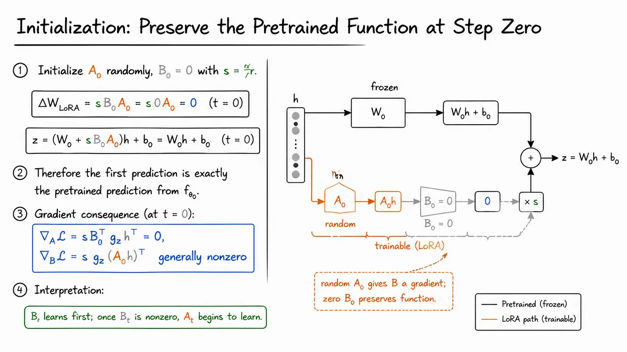
Before deciding where to insert LoRA modules in a transformer, it is worth getting one small but crucial detail right: how the LoRA parameters are initialized. This detail is easy to overlook because LoRA is often summarized as “freeze , train a low-rank update.” But if the update is initialized carelessly, the model’s behavior can change immediately before any learning has happened, destroying one of the main advantages of adaptation from a pretrained model.
Recall the LoRA parameterization for a frozen linear layer:
with
Here and are frozen pretrained parameters, is the layer input, , , and is the LoRA rank. The scalar controls the magnitude of the adaptation, often written as , so that changing the rank does not automatically make the update scale explode.
The desired behavior at the beginning of training is simple: the LoRA-augmented model should compute exactly the same function as the pretrained model at step zero. That is, before observing any task-specific gradients, we do not want the adapter to perturb the logits, hidden states, or attention projections. The pretrained model is already a highly optimized solution; LoRA should begin as a function-preserving reparameterization, not as random noise injected into a delicate computation graph.
LoRA achieves this by using an asymmetric initialization:
Then the low-rank update at initialization is exactly zero:
Therefore the layer output is also exactly the pretrained output:
This is stronger than saying the perturbation is “small.” It is not merely small in expectation, nor small under a variance calculation. It is identically zero for every input . The entire network, with LoRA modules inserted, initially represents the same function as the frozen pretrained model.
The asymmetry raises a natural question: if , have we accidentally blocked learning? The answer is no, but the gradient flow is staged. Let be the gradient arriving at the output of this linear layer. For the LoRA branch,
The gradients with respect to and are
while
which is generally nonzero as long as is not always zero and the loss gradient is nonzero.
So the first update goes into , not . This is the important subtlety: random creates nonzero features for to learn from, while zero prevents those features from affecting the model output at initialization. After one or more optimization steps, becomes nonzero, and then the gradient to ,
also becomes nonzero. In other words, learns first; once opens the path, begins to adapt as well.
This also explains why initializing both factors to zero would be a bad idea. If
then the update still preserves the pretrained function, but now
Both factors would receive zero gradient at step zero, and the LoRA branch would be stuck. Conversely, initializing both and randomly would allow gradients to flow immediately, but it would produce a random nonzero , perturbing the pretrained function before training begins. The LoRA initialization is therefore a careful compromise:
The visual summary emphasizes exactly this “safe start” structure. The frozen pretrained branch carries through and produces the original contribution . In parallel, the LoRA branch computes , but because the next factor is , the entire scaled adaptation vanishes. The two branches recombine, yet the output remains
The key intuition to keep in mind is that LoRA does not begin by changing the model. It begins by adding a trainable path whose output is exactly silent, but whose parameters are arranged so that gradients can wake it up. That is what makes LoRA a stable fine-tuning method rather than just a low-rank random perturbation of a pretrained network.
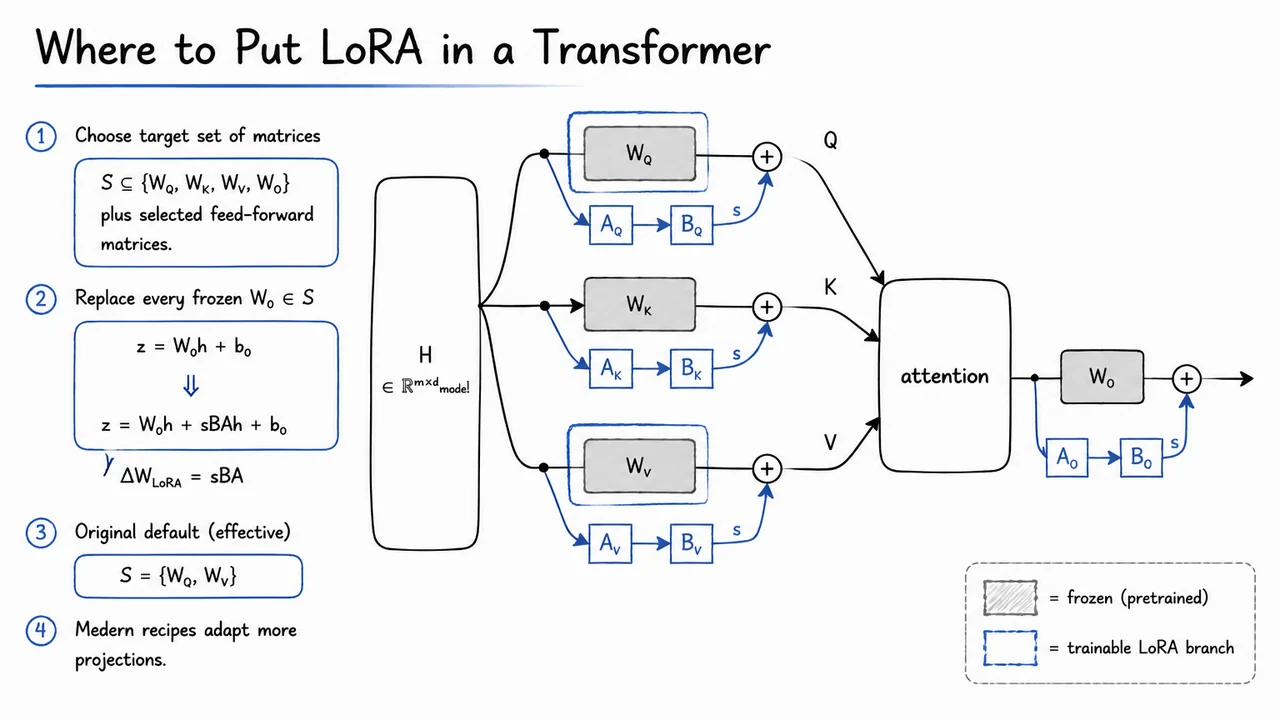
With the initialization story in place, the next question is not how to add a LoRA branch to one linear layer, but which linear layers should receive one. A transformer block contains many affine maps, and LoRA is not a new kind of transformer layer; it is a local replacement rule applied repeatedly to a chosen set of existing matrices. The practical art is choosing that set so that the adapter has enough expressive power to steer the model, without turning parameter-efficient fine-tuning back into something close to full fine-tuning.
Recall the single-layer LoRA modification. For a frozen pretrained linear map,
LoRA keeps and fixed and learns a low-rank residual update:
Here projects the input representation into a rank- adapter subspace, projects it back to the output dimension, and is a scaling factor, often written as . The key point is that this rule is matrix-local: wherever the transformer has a linear map , we can decide independently whether to attach a LoRA branch.
In a self-attention block, the most visible candidates are the four attention projections. Given hidden states , the model forms queries, keys, and values through learned projections , then applies another projection after the attention aggregation. Abstractly, LoRA asks us to choose a target set
For each , we replace the frozen map by the LoRA-augmented one:
For matrices outside , nothing changes: they remain exactly frozen and receive no trainable low-rank branch.
This choice matters because different projections control different aspects of the computation. Roughly speaking, influences what each token asks for, influences how tokens are matched, influences what information is carried forward once attention weights are chosen, and determines how the attended information is mixed back into the residual stream. Feed-forward matrices, meanwhile, often carry much of the model’s nonlinear feature transformation capacity. Adapting these locations gives LoRA different routes for changing behavior.
The original LoRA paper found that adapting only queries and values,
was often a strong default. This is intuitively appealing: modifying queries changes the attention pattern, while modifying values changes the content being routed. However, this is not a universal law. Many modern fine-tuning recipes adapt more projections, such as , and sometimes the MLP up/down/gate projections as well. The larger the target set, the more expressive the adapter becomes—but also the more parameters, memory traffic, and possible overfitting pressure it introduces.
A useful way to think about the design space is:
There is also a subtle failure mode: if is too restrictive, increasing the rank may not solve the problem. A high-rank update to the “wrong” matrices can still be less useful than a modest-rank update to the matrices where the task needs control. Placement and rank interact. LoRA’s low-rank assumption is about the needed update at a chosen location; it does not say that every downstream adaptation can be well represented by perturbing only one or two projections.
The visual below consolidates this idea as a transformer attention block with LoRA branches attached only to selected frozen projections. The gray boxes represent pretrained matrices that remain fixed. The blue side branches represent the trainable low-rank path , which runs in parallel with the frozen map and is added back to its output.
Notice especially the highlighted and projections: they mark the common original LoRA default. The same construction could be extended to , , or feed-forward matrices by adding identical low-rank side branches there too. In other words, LoRA placement is not a new derivation each time—it is the repeated application of the same constrained update rule over a chosen target set .
Once we know where LoRA is typically inserted in a Transformer—often in attention projections such as , , and sometimes or MLP matrices—the next question is more fundamental: why should a low-rank update be a reasonable restriction at all? Full fine-tuning allows every entry of a weight matrix to move independently. LoRA, by contrast, insists that the learned update must factor through a small bottleneck dimension . That is a strong constraint, so we need a mathematical reason to believe it can preserve the important part of adaptation.
Recall the contrast. In full fine-tuning, a pretrained weight matrix is changed to
where can be any matrix of the same shape. LoRA freezes and learns only a structured update
where , , and is a scalar scaling factor. Because this update passes through an -dimensional inner space, its rank is limited:
So LoRA is not merely “using fewer parameters.” It is asserting that the useful task-specific movement in weight space can be expressed, or at least well-approximated, by a matrix whose action lives in only a few dominant directions.
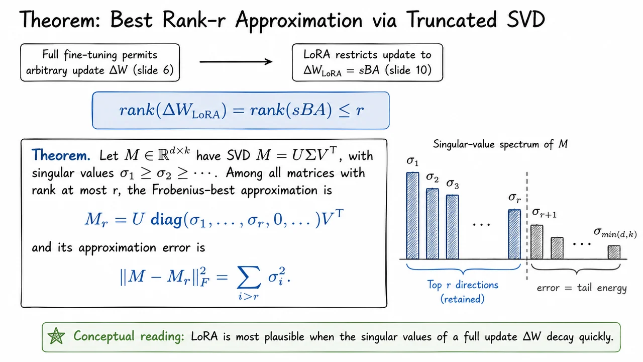
The relevant theorem is the Eckart–Young–Mirsky theorem, specialized here to the Frobenius norm. Let be any matrix, with singular value decomposition
where the singular values satisfy
The singular values measure how much “energy” or variation the matrix has along orthogonal input-output directions. Large singular values correspond to directions in which the matrix has a strong effect; small singular values correspond to weaker directions.
The theorem says that if we are allowed to approximate using only a matrix of rank at most , then the best possible approximation in Frobenius norm is obtained by keeping only the top singular values and discarding the rest:
Moreover, the approximation error is exactly the energy of the discarded tail:
This is the key bridge to LoRA. Suppose we imagine performing full fine-tuning and obtaining some update . If the singular values of decay quickly, then most of the update’s Frobenius energy is concentrated in a small number of directions. In that case, a rank- approximation may capture nearly all of the meaningful movement:
LoRA does not explicitly compute the SVD of the full fine-tuning update during training. Instead, it directly optimizes a low-rank factorization . But the theorem tells us why this is a plausible parameterization: if the true useful update is approximately low-rank, then there exists a low-rank matrix that is close to it.
There is an important subtlety here. The theorem is an approximation theorem, not a guarantee that LoRA will always match full fine-tuning. It says that low-rank approximation works well when the spectrum decays. If the desired update has many equally important singular directions, then the tail energy
may remain large, and a small-rank LoRA adapter may underfit. This is one reason the choice of rank , target modules, dataset size, and task difficulty all matter in practice.
The theorem also clarifies what LoRA is betting on:
The visual below compactly organizes this logic. The upper equation emphasizes the rank constraint imposed by the LoRA factorization . The theorem block then states the optimal low-rank approximation result: among all rank- matrices, truncated SVD gives the closest approximation in Frobenius norm.
The singular-value spectrum on the side is the conceptual heart of the result. The first bars represent the directions retained by the rank- approximation, while the gray tail represents discarded energy. When that tail is small, LoRA’s low-rank restriction is not a severe limitation; it is an efficient way to focus learning on the dominant adaptation directions.
The previous result told us what the optimal rank- approximation is: keep the top singular values and discard the rest. But for LoRA, the more important lesson is why this is true. LoRA will soon restrict a weight update to the form , which automatically has rank at most . So before we turn this into an algorithm, we want to understand the geometry of the constraint: if you are only allowed low-rank degrees of freedom, where should you spend them?
Let be the matrix we want to approximate, with singular value decomposition
where is diagonal with singular values . We compare against an arbitrary rank- candidate, written in factored form as . This notation is deliberately reminiscent of LoRA: if and , then
The proof begins with a change of coordinates. Instead of measuring the approximation error directly in the original basis, rotate both sides into the singular-vector coordinates of . The Frobenius norm is invariant under multiplication by orthogonal matrices, so
This step is powerful because it turns the target matrix into something extremely simple: a diagonal matrix . All the complexity of 's left and right singular vectors has been absorbed into the coordinate system. Meanwhile, the candidate approximation becomes . It may no longer look like a clean product , but its rank cannot increase under orthogonal rotations:
So the problem has been reduced to a more transparent one: approximate a diagonal matrix using any matrix of rank at most . In these coordinates, each diagonal entry represents the amount of energy in an independent singular direction. The Frobenius error adds squared entrywise errors, so leaving singular value unmatched costs .
The key intuition is that a rank- matrix can only fully capture independent directions. It cannot independently match all diagonal entries of if there are more than nonzero singular values. Therefore, the best strategy is obvious once we are in the right basis: spend the limited rank budget on the directions with the largest singular values, because those are the most expensive to ignore.
Formally, every rank- candidate must incur at least the squared tail energy of the singular values it cannot represent:
This inequality is the heart of the theorem. It says that no clever choice of and , no off-diagonal mixing, and no alternative coordinate trick can beat the tail energy left behind after the top singular directions are accounted for. The singular-vector basis is already the coordinate system in which the approximation problem is most clearly decomposed.
Equality is achieved by the truncated SVD approximation
for which
So the lower bound is not merely a pessimistic guarantee; it is tight. Truncated SVD attains the best possible Frobenius error among all rank- matrices.
This proof also clarifies a subtle but important point for LoRA. LoRA is not usually computing the truncated SVD of an optimal full update during training. Instead, it directly learns a low-rank update . But the SVD theorem tells us why such a parameterization can be reasonable: if the task-specific update mostly lives in a small number of dominant directions, then a low-rank factorization can capture most of its useful energy while using far fewer parameters.
The visual below compresses this argument into the essential chain: rotate into singular-vector coordinates, observe that the candidate still has rank at most , and then see the diagonal singular values split into “kept” directions and the unavoidable residual tail. The blue entries correspond to the rank budget being spent on the largest singular directions; the gray tail corresponds to the error term .
Read this picture as the bridge from linear algebra to LoRA: once updates are constrained to rank , the best possible use of that rank is to align with the most important directions of change. LoRA turns that mathematical constraint into a trainable parameterization.
Having argued that a best low-rank approximation is meaningful in the SVD sense, we can now turn that linear-algebra fact into an actual training algorithm. LoRA is not a mysterious new optimizer or a different learning objective. It is ordinary supervised fine-tuning with one structural constraint: instead of updating the pretrained weight matrix , we freeze it and learn a low-rank additive correction.
For a target linear map, suppose the pretrained layer computes
where is the input activation to that layer. Full fine-tuning would replace by , with unconstrained and the same shape as . LoRA restricts that update to factor through a small rank- bottleneck:
So the adapted layer becomes
Here projects the input activation into a low-dimensional adaptation space, and maps it back to the output dimension. The pretrained matrix remains fixed throughout training.
The scaling factor is a practical normalization convention. Since changing the rank changes the number of paths through the low-rank adapter, the scale helps keep the magnitude of the update reasonably controlled as varies. In practice, is often treated as a LoRA hyperparameter analogous to an adapter strength.
Training then minimizes the usual empirical risk over the trainable LoRA parameters , which collect all inserted factors:
The important distinction is not the loss, but the parameter set receiving optimizer updates. Gradients still flow through the network computational graph, because the LoRA factors may be deep inside a transformer block. But the optimizer state is allocated only for and , not for the original pretrained parameters .
A common initialization is asymmetric:
This makes the initial LoRA update exactly zero:
so the model begins training with precisely the pretrained function. That is a useful stability property: before seeing any task data, LoRA has not perturbed the base model at all. There is one subtle consequence: at the very first step, the gradient into is zero because it is multiplied by . The gradient into , however, is generally nonzero because is random. After moves away from zero, both factors can train normally.
The algorithm also depends on a choice of target modules . LoRA is usually not inserted into every matrix in the model. In transformer language models, common targets include attention projection matrices such as query and value projections, and sometimes key, output, or MLP projection matrices. This choice is a systems and modeling trade-off:
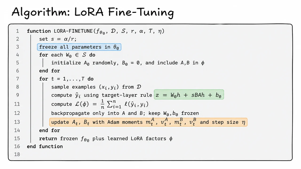
The core training loop is therefore simple. Freeze the pretrained model, attach low-rank trainable branches to selected matrices, compute predictions using the modified layer rule, evaluate the supervised loss, and update only the LoRA factors with Adam or another optimizer. The base model participates in the forward computation, but it does not accumulate trainable updates.
This is why LoRA is best understood as constrained fine-tuning, not as prompt tuning or retrieval augmentation. The model’s internal computations are genuinely modified, but only through a low-rank subspace of possible weight updates. Compared with full fine-tuning, LoRA dramatically reduces trainable parameters and optimizer memory. Compared with purely external methods, it still changes the effective network function in a task-specific way.
The visual below condenses this into the algorithmic skeleton: first freeze , then initialize one pair of low-rank factors for each selected target matrix , then run the ordinary supervised optimization loop. The highlighted layer equation
is the entire mechanism: the frozen pretrained path remains intact, while the trainable low-rank path learns the task-specific residual.
The key takeaway is that LoRA fine-tuning does not require a new learning objective or special gradient estimator. It is standard backpropagation with a carefully restricted parameterization. All of the efficiency gains follow from the fact that Adam moments, gradients, and trainable weights are maintained only for the small matrices and , while the large pretrained matrices stay fixed.
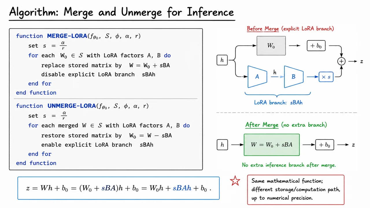
Once the adapter matrices and have been learned, LoRA has one more practical trick that is easy to miss: the trained adapter does not have to remain as a separate computational branch at inference time. During training, keeping the branch explicit is useful because stays frozen while only the low-rank factors are updated. But after training, the model only needs to compute the same function. It does not care whether the update is represented as two skinny matrices applied after , or as one already-added dense matrix.
Recall the LoRA layer during training. For a base weight , LoRA learns
with scaling
The forward pass is
Since has the same shape as , the adapter is simply an additive weight update:
So after training, we can define a merged weight
Then ordinary inference through the original linear layer gives
That equality is the entire reason merging works. The computation graph changes, but the mathematical function is the same, up to finite-precision arithmetic.
This distinction matters because LoRA’s training-time efficiency and inference-time efficiency come from different places. During training, LoRA saves optimizer state, gradient memory, and trainable parameters by freezing . During inference, however, an explicit LoRA branch would still require extra operations: compute , then , scale it, and add it to the base output. Merging folds those operations into the stored matrix once, so each future token uses the same linear layer implementation as the original model.
Operationally, the merge algorithm is almost embarrassingly simple:
set s = alpha / r
for each adapted matrix W_0:
    W = W_0 + s B A
    disable explicit LoRA branch
Unmerging reverses the operation:
set s = alpha / r
for each merged matrix W:
    W_0 = W - s B A
    enable explicit LoRA branch
Unmerging is useful when you want to continue training, swap adapters, evaluate multiple tasks on the same base model, or preserve the base model as a clean checkpoint. In practice, implementations usually track whether a layer is currently merged, because accidentally merging twice would add the adapter twice:
That kind of state bug is more common than the algebra suggests, especially when models are saved, reloaded, quantized, or wrapped by distributed training libraries.
There are also a few numerical caveats. In exact arithmetic, merge followed by unmerge restores exactly. In floating-point arithmetic, especially with low-precision weights, repeated additions and subtractions can introduce small drift. Quantized inference adds another wrinkle: if the base weight is stored in 8-bit or 4-bit form, merging may require dequantizing, adding , and possibly requantizing. That can slightly change the effective function compared with the explicit branch. The conceptual equivalence still holds, but the storage format determines how exact the implementation can be.
The key assumption behind merging is that the LoRA update is inserted as an additive linear update to a weight matrix. This is why the trick is so clean for attention projections and feed-forward projections: the adapted computation has the form
If an adaptation method inserts nonlinear operations, routing decisions, activation-dependent gates, or other input-dependent transformations, then it may not be possible to fold the adapter into a single static matrix. LoRA’s mergeability is a direct consequence of its low-rank linear parameterization.
The visual below compresses this idea into two equivalent views of the same layer. Before merging, the input flows through the frozen base path and a separate LoRA path, and their outputs are summed. After merging, the LoRA update has been absorbed into a single matrix , so inference uses the ordinary linear layer again.
The important takeaway is not merely that merging saves a few operations. It means LoRA can behave like a lightweight training-time modification while leaving behind a deployment artifact that looks like a normal dense model. That is why LoRA is attractive in production settings: adapters are cheap to train and store, but once selected for a task, they can be folded into the model so there is no extra inference branch after merge.
Once merging has made the inference story clean, the next question is the systems one: what exactly did LoRA buy us, and where did the costs move? The answer is not simply “fewer parameters” in the abstract. LoRA changes the accounting of trainable state, optimizer memory, and training-time compute, while leaving the merged inference path essentially identical to the original dense layer.
Consider one pretrained weight matrix . Full fine-tuning makes every entry trainable, so the number of trainable parameters for this matrix is
LoRA instead freezes and learns a low-rank update
where , , and . The number of trainable parameters is therefore
So the parameter fraction is
This ratio is the basic systems lever. When and are large and is small, can be tiny. For example, if and , then
or about of the dense matrix’s parameter count. That is the core reason LoRA can make adaptation of very large models practical: the fine-tuning problem no longer requires storing gradients and optimizer statistics for every pretrained weight.
The memory consequence is especially important because training memory is not just parameter memory. For each trainable parameter, we may store the parameter itself, its gradient, and optimizer state such as Adam’s first and second moments. Abstractly, we can write the trainable-state memory as
where is the number of trainable parameters, summarizes parameter and gradient storage, and summarizes optimizer state. Under full fine-tuning,
whereas under LoRA,
If the same precision and optimizer are used, the trainable-state memory fraction is again approximately .
There are a few assumptions hiding in this clean accounting. The frozen base weights still have to live somewhere during training; LoRA does not make the pretrained model disappear. Activations, attention caches, temporary buffers, communication overhead, and framework-level bookkeeping can dominate in some regimes. So is best understood as the reduction in trainable parameter state, not necessarily the exact reduction in total GPU memory. Still, for large models trained with optimizers like Adam, removing optimizer state for the frozen weights is often a major win.
Compute has a slightly different story. During training, LoRA usually evaluates the frozen dense path and the low-rank branch separately:
The base multiplication costs on the order of multiply-adds for one input vector . The LoRA branch can be evaluated as followed by , costing
additional multiply-adds. This is small relative to when is small, but it is not zero. LoRA saves dramatically on trainable state, while adding a modest training-time branch.
The merge operation is what prevents that branch from becoming an inference penalty. After training, we can form
and then compute the layer as the ordinary dense affine map
At that point, the deployed model no longer needs to explicitly compute , then , then add the result to . The adaptation has been absorbed into the dense weight. This is why LoRA is often described as having no additional inference latency after merging, assuming the merged matrix is materialized and served like any other weight.
The main takeaway is a separation of concerns:
The subtle failure mode is to confuse these three budgets. A method can be cheap in trainable state but still require the full frozen model in memory. It can reduce optimizer memory while leaving activation memory unchanged. It can add a branch during training but remove that branch at inference. Good systems accounting keeps these categories separate instead of collapsing them into a single claim like “LoRA is cheaper.”
The visual below compresses this accounting into two complementary views. The left side treats LoRA as a parameter and memory calculation: full fine-tuning pays for trainable entries, while LoRA pays for only , giving the fraction . The right side treats LoRA as a computation graph: during training, the input flows through both the frozen base path and the low-rank adaptation path.
The final part of the visual emphasizes the operational payoff of merging. Before merging, the LoRA factors and are explicit modules in the forward pass. After MERGE-LORA, the model serves a single dense matrix , so the low-rank branch is no longer on the inference path.
After accounting for parameters, memory, and latency, it is tempting to treat LoRA as “just add two small matrices.” Algebraically, that is almost true. Operationally, it is not. A LoRA layer is correct only if the frozen path, low-rank path, scaling convention, optimizer state, and merge state all agree with one another. Many failed LoRA runs are not failures of the low-rank hypothesis; they are bookkeeping errors that quietly change the effective model being trained.
For a pretrained linear map , LoRA replaces direct fine-tuning of with a constrained update
where , , and . The forward pass is therefore
The crucial implementation detail is that is not merely “not optimized in spirit”; it must be frozen in the computational graph and excluded from the optimizer. If accidentally receives gradients or optimizer state, then the model is no longer doing LoRA fine-tuning. It is doing full or partial fine-tuning plus a low-rank side update, which changes both the memory accounting and the experimental interpretation.
The scale is another small detail with large consequences. Without it, increasing the rank changes not only the expressivity of the update but also its typical magnitude. That makes rank comparisons misleading: a higher-rank adapter may appear better simply because it is allowed to produce larger updates. The usual convention keeps the effective update scale controlled as varies, so that changing more cleanly probes capacity rather than accidentally changing the learning dynamics.
Target selection also matters. LoRA is not automatically attached to every matrix in the network. One chooses a set of target matrices : for example attention query and value projections, sometimes key and output projections, and in some models MLP projections as well. Each adapted matrix with shape contributes
trainable parameters, so the memory cost scales linearly with the number and shapes of selected targets. A small rank applied broadly can cost more than a larger rank applied selectively. This is why LoRA design is partly an architectural choice, not only a numerical one.
Dropout introduces another subtle branch-specific distinction. If LoRA dropout is used, it is usually applied only to the adapter input, not to the frozen pretrained path:
This preserves the deterministic pretrained computation while regularizing the learned update. Applying dropout to the whole input , or to both branches, changes the behavior of the frozen model itself and can degrade the very prior that LoRA is trying to preserve.
Bias terms deserve similar care. In the basic LoRA formulation, the pretrained bias remains frozen along with . Some implementations optionally train biases, but then those biases are part of the trainable parameter set , and the method is no longer the minimal “only ” variant. That may be perfectly reasonable, but it should be a deliberate experimental choice rather than an accidental default inherited from a framework.
The optimizer should also be configured for the adapter parameters, not for the original model. Adam statistics, learning rates, weight decay, and precision handling should apply to and only, unless additional trainable parameters have been explicitly enabled. A common bug is to freeze gradients but still pass too many parameters to the optimizer, or to create optimizer state before freezing. In large models, that mistake can erase much of LoRA’s memory advantage even if the numerical updates to are zero.
Finally, merging requires exact state bookkeeping. During training or adapter-based inference, the computation uses the separate form . For deployment, one may merge the adapter into the base weight:
If we later want to resume adapter training or switch adapters, we must unmerge exactly once:
Merging twice, forgetting that a layer is already merged, or unmerging with a different adapter state can silently corrupt the base weights. A robust implementation therefore tracks whether each adapter is currently merged and treats merge/unmerge as inverse operations, not as informal convenience calls.
A good mental checklist for LoRA implementation is:
The visual below condenses these decisions into a comparison table: each row corresponds to a choice that looks minor in code but changes the mathematical object being trained. The highlighted scaling row emphasizes that and should be interpreted together, while the warning strip collects the most common implementation bugs: missing the scale factor, accidentally updating , and merging without consistent inverse bookkeeping.
Read the table as a systems-level companion to the formula . The equation defines the adapter; the implementation choices define whether the code actually realizes that adapter.
After all the implementation details—where to insert adapters, how to scale them, how to initialize them, and how to merge them—it is useful to step back and test the central LoRA claim in the cleanest possible setting. The claim is not merely that LoRA uses fewer parameters. The stronger claim is that, when the needed change to a pretrained model is intrinsically low-rank, LoRA can represent that change exactly once the chosen adapter rank is large enough.
Consider a synthetic linear adaptation problem. We start with a frozen pretrained weight matrix , and the data are generated by a true adapted model
Here is the input matrix, is the target output matrix, is the unknown task-specific update we wish we could apply to , and is noise. The important design choice is that has rank exactly . This makes the LoRA hypothesis testable: if the target adaptation is truly rank-2, then a LoRA adapter of rank should be expressive enough to recover it, up to noise and optimization error.
LoRA does not train directly. Instead, it freezes and learns a low-rank update
If , then typically
so has rank at most . The scalar controls the effective scale of the learned update, but it does not change the rank. Therefore the representational question is simple: can a rank- matrix equal the true update ?
When , the answer is no in general. Since
a rank-1 LoRA adapter can only capture one independent adaptation direction. But the ground-truth update has two independent directions. Even with unlimited data and perfect optimization, one component of must be left out. This is a representation error, not merely a training failure.
The best possible rank-1 approximation to is given by truncated SVD. If
has two nonzero singular values , then the optimal rank-1 approximation keeps only the top singular component. The unavoidable squared Frobenius error is
This equation is the cleanest way to see what rank mismatch costs. The rank-1 adapter is not “almost LoRA enough” unless the second singular value is tiny. If is substantial, the missing direction produces a visible loss gap.
Once , the situation changes qualitatively. Because itself has rank , there exists a factorization of through a two-dimensional bottleneck. For example, using the compact SVD , we can choose factors of rank so that
One valid construction is to absorb the singular values and scaling into the factors, such as
or any equivalent rescaling. More generally,
So in this synthetic example, LoRA’s expressivity becomes exact at . Increasing the rank beyond does not improve the best achievable noiseless fit, because there is no additional signal direction to capture.
That does not mean the training loss becomes zero. The data contain noise , so even the correct model class cannot explain every observed target perfectly. Once , the remaining error should be governed by the noise floor and by optimization details, not by the rank constraint. This distinction is important in real experiments too: a plateau in validation or training loss after increasing may indicate that rank is no longer the bottleneck.
This example also clarifies a common failure mode. If LoRA underperforms at small rank, that does not automatically mean the method is broken; it may simply mean the chosen rank is below the intrinsic rank of the needed update. Conversely, if increasing beyond some point yields little benefit, the task adaptation may already be well captured by a low-dimensional subspace, or other bottlenecks—data quality, optimization, regularization, placement of adapters—may dominate.
The visual below compresses this reasoning into a single experiment: generate data from a frozen plus a true rank-2 update , then fit LoRA adapters with ranks . The predicted curve is not gradual in the idealized setting. It should show a sharp drop when the LoRA rank reaches the true rank, followed by a plateau near the noise floor induced by .
The key takeaway is therefore very concrete: LoRA succeeds exactly in this synthetic setting once its rank reaches the true rank of the required weight update. Rank misses a direction; rank can represent the target update; larger ranks mostly add unused capacity unless noise, finite data, or optimization behavior makes them matter.
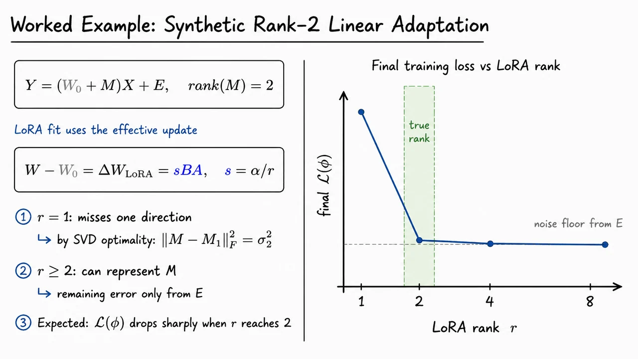
The synthetic rank-2 example was deliberately stripped down: one linear map, one desired low-rank correction, and a clean demonstration that LoRA can learn the update without touching the pretrained matrix. The same logic becomes more useful when we place it inside a transformer block, because transformer layers contain several large linear projections repeated many times across depth. The practical question is not merely can we write , but which matrices should receive so that the adaptation is expressive without becoming another form of full fine-tuning?
A common and effective choice is to adapt selected attention projections, especially the query and value projections. In a standard attention block, hidden states are projected into queries, keys, and values:
Here is the batch-and-sequence collection of hidden states, often represented as a row-vector matrix of shape roughly . The matrices map from the model hidden dimension into attention-space representations. LoRA does not change the fact that attention is computed from , , and ; it only changes how some of those projections are produced.
For this worked example, we choose the target set
That means and remain frozen pretrained matrices, but each receives its own trainable low-rank correction. The key projection , the output projection , the feed-forward layers, layer norms, residual connections, and attention softmax are all left structurally unchanged in this simplified placement rule. This is important: LoRA is not inserting a new transformer submodule. It is modifying selected linear maps by adding a parallel low-rank branch.
For the query projection, the adapted computation becomes
Similarly, for the value projection,
Strictly speaking, the and used for are distinct trainable parameters from the and used for . We often write the same symbols because the parameterization is the same, but each adapted matrix owns its own LoRA factors. The frozen matrix supplies the pretrained behavior; the learned product supplies the task-specific displacement; and the scalar , often , controls the scale of that displacement.
For a single token vector , the same idea is easier to read in column-vector form:
This expression reveals the computational structure. The token first follows the original frozen path . In parallel, it passes through a rank- bottleneck: maps the hidden vector into a smaller -dimensional space, and maps it back to the output dimension. The two paths are then added. Because has rank at most , LoRA can only express updates inside a low-dimensional subspace of all possible weight changes—but that constraint is precisely what makes it parameter-efficient and regularizing.
There are a few subtle implementation details worth keeping straight. First, adapting and changes the behavior of attention in different ways. A query update changes what each token asks for when attending to the sequence; a value update changes what information is carried back once attention weights have selected positions. This pairing often gives strong downstream performance because it can alter both the addressing mechanism and the retrieved content. By contrast, leaving fixed means the representation being matched against queries remains anchored to the pretrained model’s key space.
Second, LoRA preserves the surrounding computation graph. There are:
This matters operationally. During training, only the LoRA factors receive gradients. During inference, the low-rank update can either remain as a small side branch or be merged into the frozen weight by replacing with . After merging, the runtime computation is just an ordinary dense projection again.
The main failure mode to keep in mind is under-allocating rank or adapting too few modules. If the downstream task requires a broad reconfiguration of the representation space, a tiny low-rank correction on only and may not provide enough capacity. On the other hand, increasing the rank or adapting many more projections gradually trades away the parameter-efficiency advantage. LoRA’s empirical success comes from the observation that many useful task adaptations appear to occupy a much lower-dimensional subspace than the full parameter space would suggest.
The visual below consolidates this placement rule inside one attention block. The hidden states feed the usual projection matrices, but only and receive orange low-rank side branches. The key and output projections remain gray and unchanged, reinforcing the point that the transformer architecture is not being rebuilt around the adaptation.
The equation panel in the visual is the compact algebraic summary: for selected projections, replace by ; for unselected projections, keep the pretrained matrix as-is. In other words, LoRA’s intervention is local, additive, and low-rank: the base attention computation remains intact while the task learns small trainable corrections exactly where we choose to attach them.
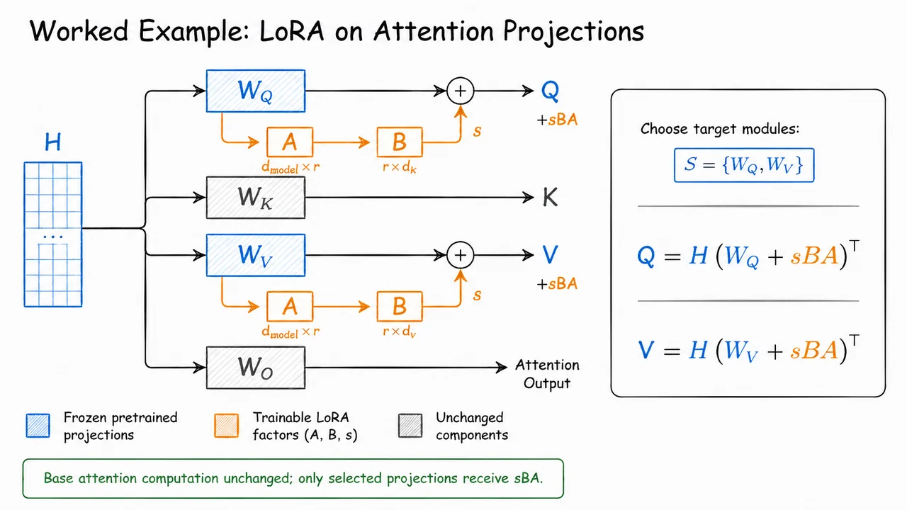
After working through a concrete attention-projection example, it is worth stepping back and noticing what LoRA really gives us: not merely a smaller set of trainable matrices, but a controlled adaptation budget. We freeze the pretrained model as the stable computational backbone, then decide where and how much freedom to give the model through low-rank residual updates.
That distinction matters because LoRA is not uniformly powerful everywhere. A low-rank update can only express changes that lie in a small-dimensional subspace. If the task mainly requires redirecting existing features—changing which tokens attend to which others, or slightly reshaping an already useful representation—then a small adapter can be surprisingly effective. But if the task requires learning entirely new internal features, new reasoning routines, or domain-specific transformations absent from pretraining, the low-rank constraint may become a real bottleneck.
In practice, a LoRA configuration is defined by a few coupled choices:
The most common insertion points are attention projections, especially and . This is not accidental. Query and value projections directly affect where information is retrieved from and what content is passed forward. For many instruction-following or task-adaptation settings, modifying these projections gives the model enough behavioral flexibility without touching every dense layer.
But this is also an assumption. If the adaptation requires changing token mixing, output composition, or feed-forward feature transformations, then limiting LoRA to and may underfit. Adding adapters to , , or MLP matrices increases capacity, but it also increases trainable parameters, optimizer memory, and potentially training instability. LoRA’s efficiency is therefore not just a theorem about low rank; it is an empirical design trade-off.
A useful way to think about the rank is that it controls the number of independent “directions of change” available to the update. Small ranks often work because fine-tuning gradients in large pretrained models are empirically structured: many useful adaptations appear to live in low-dimensional subspaces. However, this is not guaranteed. If is too small, the adapter cannot represent the needed update. If is too large, LoRA begins to lose its parameter-efficiency advantage and can overfit, especially on small datasets.
There is also an important deployment distinction. During training, the model computes the frozen path and the adapter path separately. At inference time, however, the adapter update can often be merged into the frozen weight, producing an effective weight matrix with no extra adapter computation. This is one reason LoRA is attractive operationally: it can behave like a lightweight fine-tuning method during training while still allowing ordinary dense inference afterward.
The main failure mode is forgetting that LoRA is a constrained update, not magic compression. Its success depends on the pretrained model already containing reusable structure. LoRA is strongest when the task is close enough to pretraining that adaptation can be expressed by recombining or redirecting existing capabilities. It is weaker when the task demands large architectural, representational, or domain shifts.
The visual below serves as a compact map of these ideas: the frozen model remains the center of gravity, while small trainable adapters are inserted only at selected locations. The key intuition is that LoRA lets us choose a thin path for learning through a very large network, rather than reopening every parameter.
It also prepares us for the next question: once we have this design space, which choices actually matter most? Rank, target modules, and inference latency are not independent details; they are the knobs that determine whether LoRA is merely cheap, genuinely effective, or both.
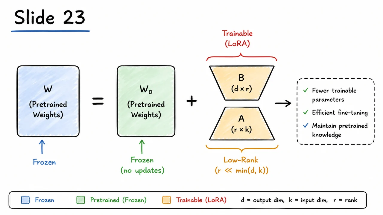
A useful way to make LoRA feel less like a trick and more like an engineering tool is to ask a practical question: if the adapter is cheap, how cheap should we make it? The low-rank update gives us a knob, the rank , but that knob does not behave like an ordinary “more is always better” hyperparameter. Empirically, LoRA often enters a regime where task quality has mostly saturated while cost continues to grow predictably. The art is to stop increasing capacity when the model has enough adaptation freedom, rather than when the adapter is as large as we can afford.
For a single adapted weight matrix , LoRA replaces a dense trainable update with a factorized update , where and . The number of trainable LoRA parameters is therefore
Here is the fraction of parameters trained relative to full fine-tuning of that matrix. The important structural fact is that LoRA cost grows linearly in , while the full matrix has degrees of freedom. When , the adapter is a small subspace of possible dense updates.
This linear dependence makes rank ablations especially interpretable. If we double , we roughly double the number of trainable adapter parameters for that matrix. We also roughly double the optimizer state associated with those parameters. A simple training-memory proxy is
where accounts for storing trainable parameters and accounts for optimizer state such as Adam moments. The frozen base weights still occupy memory, of course, but the additional trainable state scales with the LoRA adapter size. This is one of the main reasons LoRA is attractive: it decouples adaptation capacity from the full parameter count of the pretrained model.
The subtle point is that accuracy does not usually grow linearly with . A common empirical pattern is:
This is not guaranteed for every task, dataset, or model, but it is a strong practical prior. LoRA works best when the downstream adaptation is intrinsically lower-dimensional than the full weight space. If the task requires broad changes across many features, layers, or attention pathways, increasing may continue to help for longer. If the task is close to the pretraining distribution, small ranks can be surprisingly competitive.
The second ablation knob is where to insert LoRA. In Transformer attention blocks, a strong default is often
meaning that LoRA adapters are placed on the query and value projection matrices. This choice is popular because it gives the model direct control over what tokens attend to and what information is transmitted through attention, while keeping the adapter budget small. Expanding the target set to include more projections, such as
can improve performance on harder tasks, but it increases proportionally to the number and size of adapted matrices. The same trade-off applies if LoRA is added to MLP projections: more insertion points mean more adaptation capacity, but also more trainable parameters, optimizer state, and training compute.
This creates a useful diagnostic distinction. If performance is poor with a small rank and narrow target set, the model may be under-adapted. But the remedy is not always “increase rank.” Sometimes adding LoRA to additional modules is better than making the same modules higher rank. Rank controls the expressiveness of each local update; target-module selection controls where in the computation graph the model is allowed to change. A small adapter in the right place can beat a larger adapter in the wrong place.
Latency introduces a final practical wrinkle. During unmerged LoRA training, the forward pass through an adapted linear layer has two contributions: the frozen base projection and the low-rank residual. Schematically, the model computes both and , then adds them. That extra branch is usually acceptable during training, especially because is small, but it is still an additional computation.
At inference time, LoRA has a clean escape hatch: merge the adapter into the base weight. After merging, the adapted layer is just
This is algebraically equivalent to the unmerged computation, up to numerical precision, but it removes the separate adapter branch. The deployed model can therefore run like an ordinary dense model with modified weights. This is why LoRA can offer parameter-efficient training without necessarily imposing extra inference latency, provided the adapters are merged before serving.
The practical rule is simple: start small, then expand only when the ablation says you are underfitting. A reasonable workflow is:
The visual below compresses these ablation lessons into one picture. The central empirical pattern is the mismatch between the blue accuracy curve and the orange parameter-cost line: accuracy may rise quickly and flatten, while keeps increasing linearly with . That gap is exactly where LoRA’s efficiency decision lives. We are not looking for the largest adapter; we are looking for the smallest adapter that reaches the plateau.
The target-module bars summarize the second axis of the search: is the compact baseline, while adding more attention projections expands capacity at additional cost. The merge schematic captures the deployment story: unmerged LoRA is a two-branch computation during adaptation, but after merging it becomes the single dense expression . Together, these ablations support the core recipe: tune rank and insertion sites for accuracy, but merge for inference so that parameter-efficient training does not become unnecessary serving overhead.
The ablations make an important point that is easy to miss: LoRA is not a universally “small version” of full fine-tuning. It is a structured hypothesis about what kind of change the pretrained model needs. When the rank, target modules, and scaling choices line up with the task, LoRA can look almost magically efficient. When they do not, the same mechanism can become a bottleneck.
At the center of the limitation is the low-rank constraint itself. For a frozen pretrained weight matrix , LoRA replaces full fine-tuning of with
where
Because the update factors through an -dimensional bottleneck, its rank is bounded:
This is exactly why LoRA is parameter-efficient, but it is also exactly why it can fail. If the task requires a genuinely high-rank change to some weight matrix, then no optimizer can recover that update from a rank- parameterization. Increasing training time or tuning the learning rate will not remove the geometric constraint. The best LoRA can do is find a good low-rank approximation to the desired update.
This connects back to the rank-2 toy example: LoRA succeeds cleanly when the needed movement in parameter space is itself low-dimensional. In large pretrained models, this is often a reasonable assumption because many downstream tasks reuse most of the pretrained representation and only need to steer a relatively small number of features. But “often” is not “always.” Some tasks may require broad changes across many features, layers, or attention pathways. In those cases, a small rank may underfit even if the training loss appears stable.
A second failure mode is placing the adapter in the wrong part of the network. LoRA does not adapt every frozen weight unless we explicitly choose to insert it everywhere. We usually define a target set , such as the query and value projection matrices and in attention layers. If the task-relevant change lives mostly in , , MLP projections, embeddings, or later normalization-sensitive pathways, then adapting only and may leave performance on the table. In this sense, LoRA’s efficiency comes not only from low rank, but also from a sparsity assumption over which modules need to move.
There is also a more practical limitation: LoRA has fewer trainable parameters, but it does not eliminate the frozen model. At inference time we still need access to , either explicitly or after merging the update into it. For very large models, storing the frozen base can dominate the memory footprint. This is why LoRA is often paired with quantization: keep the large frozen backbone in low precision, and train or store the low-rank adapter separately. Methods in this family preserve LoRA’s adaptation efficiency while attacking the memory cost that LoRA alone does not solve.
The hyperparameters are another source of fragility. The scaling , adapter dropout , optimizer choice, learning rate , and initialization all influence the effective size and stability of the update. A common mistake is to treat LoRA rank as the only meaningful knob. In practice, rank, scale, dropout, and target modules interact. For example:
Finally, some extensions modify the parameterization itself. Standard LoRA writes the update as , which couples the direction of the update with its magnitude through the same learned factors. Decomposition variants try to separate or reweight these roles, or allocate rank adaptively across layers. The common theme is not to abandon LoRA’s frozen-base-plus-trainable-update template, but to relax one of its bottlenecks: fixed rank, fixed target modules, fixed scaling behavior, storage cost, or the particular factorization.
The visual below condenses these limitations into a comparison: each weakness of the basic LoRA recipe corresponds to a natural family of extensions. High-rank tasks motivate larger or adaptive ranks; poor target selection motivates expanding ; memory pressure motivates quantized frozen bases; sensitivity to , , and motivates systematic ablations rather than fixed defaults.
The key takeaway is that LoRA is powerful when the desired update is both low-rank and placed where the model needs to change. Its extensions are best understood as ways of making that assumption less brittle, while preserving the central advantage: most of the pretrained network remains frozen, and only a compact adaptation mechanism is trained.
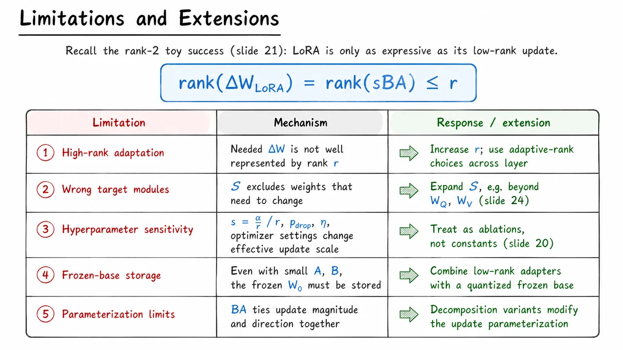
After looking at the limitations and extensions, it is useful to step back and name the common structure underneath all of these methods. The original problem was never merely that fine-tuning works poorly; full fine-tuning often works very well. The problem is that, for large pretrained models, it asks us to store and optimize a nearly complete copy of the model for every downstream task. If the base parameters are , full fine-tuning replaces them with task-specific parameters , and in each adapted linear layer we can write the change as
That equation is the organizing lens for the whole lecture. Fine-tuning says: “learn an unrestricted .” Parameter-efficient adaptation asks: “can we get most of the benefit of , while making the trainable object much smaller?”
For a single dense matrix , full fine-tuning trains every entry of the update. The adapted computation is ordinary linear inference:
and the trainable parameter count for that matrix is
This is maximally flexible, but it scales badly when we replicate it across many layers, many tasks, and many deployment variants. The inefficiency is not only storage; it also affects optimizer memory, checkpoint management, multi-task serving, and the operational burden of deciding which full model copy should be loaded for which request.
The alternatives differ mainly in where they place the small trainable object . Prompt and prefix methods keep the model weights frozen and instead alter the input-side or attention-side context. They can be extremely compact, but their adaptation is mediated through tokens or attention states rather than through the internal weight matrices themselves. This can introduce sequence-length or attention overhead, and the adapted behavior is not usually mergeable into the original weights.
Adapters choose a different compromise: they insert small trainable modules between frozen layers. These modules often use a bottleneck structure, so the number of trainable parameters remains modest. But the adapted computation is no longer exactly the original network graph. Even if the base model is frozen, inference now includes extra module calls, which can add latency and complicate deployment. Adapters are powerful because they introduce new nonlinear computation; they are less attractive when the goal is to preserve the original architecture and recover a single ordinary weight matrix at inference.
LoRA occupies a particularly elegant point in this design space. It keeps the full fine-tuning viewpoint that adaptation is an additive weight update, but restricts that update to a low-rank factorization. For selected matrices , LoRA uses
where , , and . The adapted computation becomes
The key is that LoRA does not need to train the full matrix. It trains only the two skinny factors, so the per-matrix trainable parameter count is
which is much smaller than when is small.
This is why LoRA is best understood not as a mysterious new module, but as a rank-constrained version of full fine-tuning. It says that the task-specific displacement in weight space does not need to point in an arbitrary -dimensional direction. Instead, useful adaptation often lies in a much lower-dimensional subspace. The assumption is empirical but plausible: pretrained models already contain rich features, so many downstream tasks may require coordinated changes along relatively few directions rather than independent changes to every scalar weight.
There are two important subtleties. First, low rank is a constraint on each adapted matrix update, not necessarily on the entire function learned by the network. When LoRA is inserted into many layers, the resulting functional change can still be expressive because these low-rank perturbations compose through the nonlinear transformer. Second, LoRA’s efficiency depends on choosing the insertion set wisely. Applying LoRA to attention projection matrices is common because those matrices strongly control routing and representation mixing, but different tasks and model families may benefit from adapting MLP projections, output projections, or additional layers.
The deployment story is what makes LoRA especially attractive. During training, we compute the frozen path and the low-rank residual . After training, however, the update can be merged:
Once merged, inference uses an ordinary dense matrix multiplication again. There is no extra adapter module, no extra prompt length, and no need to evaluate the low-rank branch separately unless we want to keep adapters dynamically swappable. This mergeability is one of LoRA’s defining practical advantages: it behaves like a compact training-time parameterization but can become standard weights at serving time.
The final comparison is therefore not “which method is universally best?” but rather “which compromise matches the constraint?” A useful summary is:
The visual summary that follows compresses this whole design space into one table. Each row answers the same questions: what is trained, how the forward computation changes, how many parameters are introduced, whether inference becomes more expensive, and whether the adaptation can be folded back into ordinary weights.
The LoRA row is the important synthesis. It connects the full fine-tuning equation to the constrained update , shows the parameter reduction from to , and highlights the merge operation . In one line, it captures the central takeaway of the lecture: LoRA is full fine-tuning’s additive matrix update, restricted to a trainable low-rank factorization that is cheap to optimize and recoverable as ordinary weights for inference.
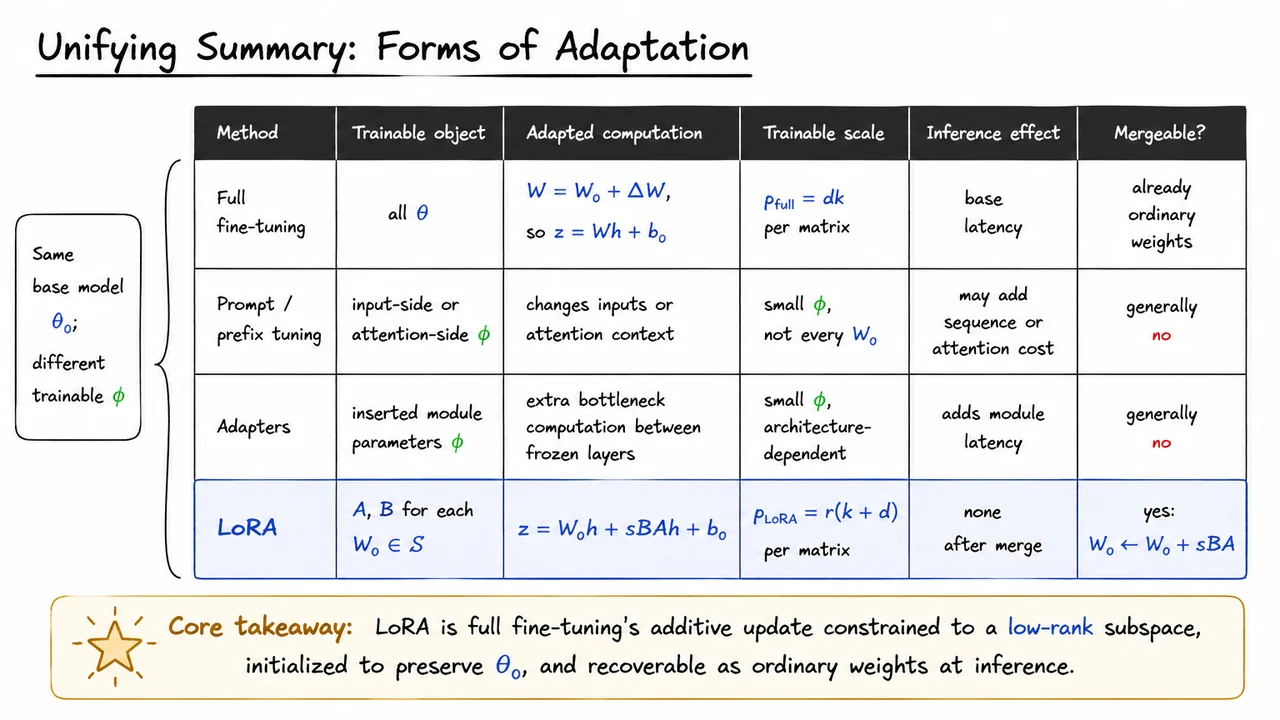
Before we get to LoRA itself, it is worth slowing down on the pressure point that made methods like LoRA necessary. Modern pretrained models are powerful precisely because they concentrate enormous general-purpose knowledge into a parameter vector . But that same scale turns the most obvious adaptation strategy—just fine-tune everything—into a systems problem as much as a learning problem.
Suppose we start with a pretrained model and a supervised downstream dataset
For a task such as sentiment classification, medical extraction, instruction following, or customer-specific generation, adaptation means changing something about the model so that its predictions better match the desired outputs . Abstractly, we choose some trainable parameters and minimize the empirical loss
The important detail is that does not have to be the entire model. It simply denotes whatever parameters we decide are allowed to move during adaptation. In full fine-tuning, we make the maximal choice: initialize , set , and optimize every parameter of the pretrained model.
This is a very strong baseline. Full fine-tuning gives the optimizer direct access to every layer, every attention projection, every MLP weight, every embedding table, and every normalization parameter. If the downstream task needs a subtle redistribution of features throughout the network, full fine-tuning can in principle make those changes. That flexibility is one reason it often performs well when we have enough data, compute, and careful regularization.
The bottleneck is that flexibility is expensive. A model with billions of parameters is not just expensive to pretrain; it is expensive to repeatedly copy, optimize, store, serve, version, and audit. During training, full fine-tuning typically requires optimizer state for every trainable parameter. With Adam-like optimizers, that can mean storing the parameter, its gradient, and multiple moment estimates. The memory footprint can become several times larger than the model weights alone.
The deployment cost is even more direct. If we fine-tune a separate full model for each task or customer, then each adaptation produces another full-sized parameter vector:
Even if each differs only slightly from the original , naive full fine-tuning stores every adapted copy independently. For a 7B, 13B, or 70B parameter model, this quickly becomes impractical. The problem is not merely training one model once; the problem is supporting many adapted models.
There is also a statistical subtlety. Downstream datasets are often much smaller than the pretraining corpus. When is small and has billions of trainable degrees of freedom, the model has enough capacity to memorize idiosyncrasies of the task dataset. Good fine-tuning practice therefore relies on learning-rate schedules, regularization, early stopping, validation sets, and sometimes freezing parts of the network. Full fine-tuning is powerful, but it is not automatically data-efficient or operationally convenient.
This motivates the central question behind parameter-efficient fine-tuning:
> Can we keep the pretrained weights frozen, while letting a much smaller set of parameters carry the task-specific adaptation?
If the answer is yes, then we can reuse one large shared model and store only a small task-specific delta for each downstream use case. Instead of maintaining many full copies of , we maintain one base model plus many compact adaptations. LoRA will instantiate this idea by restricting the update to certain weight matrices and forcing that update to have low rank, but the motivation starts here: most of the pretrained model should remain a reusable shared asset.
A useful way to frame the trade-off is:
The visual below compresses this argument into a left-to-right bottleneck: a small task dataset feeds into a huge pretrained model, full fine-tuning produces separate large adapted models, and the cost grows with the number of tasks or customers. The key asymmetry is that the task data and desired behavioral change may be small, while the object being duplicated is enormous.
The small placeholder in the diagram points toward the idea LoRA will develop next. Instead of asking every parameter in to move, we will ask whether adaptation can live in a much lower-dimensional space—small enough to store and train cheaply, but expressive enough to recover much of the performance of full fine-tuning.
The optimization view from the previous section makes full fine-tuning look deceptively simple: start from a pretrained parameter vector , optimize the downstream loss, and obtain an adapted parameter vector . Conceptually, that is clean. Operationally, however, it hides the main scaling problem: after fine-tuning, is no longer a universal shared object. It is now task-specific.
If we adapt the same pretrained model to one downstream task, this may be acceptable. But the whole point of large pretrained models is that they are reused across many tasks: summarization, code generation, retrieval-augmented QA, domain-specific chat, instruction following, classification, extraction, and so on. With full fine-tuning, adapting one base model to 100 downstream tasks gives 100 distinct full model checkpoints. Each checkpoint contains a complete copy of the model parameters, even if the actual task-specific change from is small.
For a single dense weight matrix , full fine-tuning treats every entry as trainable. The number of trainable parameters in that matrix is therefore
This looks harmless at the matrix level, but modern transformers contain many such matrices: attention projections, MLP projections, embeddings, output heads, and normalization-related parameters. Full fine-tuning scales with the size of the entire model, not with the amount of information needed to specialize the model to the task.
The training memory cost is even worse than the checkpoint size suggests. During training, we do not only store the parameters themselves. We also store gradients, activations needed for backpropagation, and optimizer state. For Adam-like optimizers, each trainable parameter typically carries additional moment estimates, often the first and second moments. Abstracting away implementation details, the memory footprint associated with trainable parameters can be summarized as
where accounts for storing trainable weights and related parameter-level quantities, while accounts for optimizer state. The important point is not the exact constant; it is the scaling. If every parameter is trainable, Adam allocates optimizer state for every parameter.
This creates a practical failure mode that is easy to underestimate. The base model may be shared in theory, but full fine-tuning destroys that sharing in deployment. Each task now needs its own full checkpoint. Serving many variants requires model routing, checkpoint loading, memory residency decisions, version management, and duplicated storage. If the base model has billions of parameters, even “just one more fine-tuned task” can become expensive.
The key inefficiency is that full fine-tuning assumes the task-specific solution must be represented as an entirely new point in the full parameter space. But empirically, many downstream adaptations appear to require only a comparatively small change in behavior. We would like to capture that change without rewriting and storing the entire model. In other words, the desired pattern is:
This is the motivation behind parameter-efficient fine-tuning. Rather than asking, “How do we find a new full model for each task?”, we ask, “Can we represent the task-specific update compactly?” LoRA will answer this by constraining updates to certain weight matrices to have low rank, but before getting there, it is important to see the failure case clearly: full fine-tuning pays the full model cost even when the useful adaptation may be much smaller.
The visual below compresses this contrast into two patterns. On the left is the full fine-tuning regime: one shared pretrained model gives rise to many separate full checkpoints, with storage and Adam state growing with the full parameter count. On the right is the parameter-efficient goal: keep frozen and shared, while attaching small task-specific parameters .
The equation at the bottom anchors the intuition mathematically. For a fully trainable matrix, , and the training footprint scales like . The rest of the lecture is about replacing that scaling law with something much smaller, while preserving most of the quality benefits of fine-tuning.
The “one full copy per task” failure mode suggests a natural repair: stop treating every downstream task as a reason to duplicate the whole model. If the pretrained parameters already encode broadly useful linguistic, visual, or multimodal structure, then perhaps task adaptation should be a small correction rather than a complete rewrite. This is the core motivation behind parameter-efficient fine-tuning: keep the base model frozen, and learn only a comparatively tiny set of task-specific parameters .
In abstract form, most PEFT methods follow the same pattern:
This changes the economics of fine-tuning. Instead of storing and serving a separate full model for each task, we store one shared pretrained backbone plus many small task modules. Training also becomes cheaper because gradients, optimizer states, and parameter updates are needed only for , not for the full . For very large models, this distinction is not cosmetic: optimizer states alone can multiply memory requirements several times over the raw parameter count.
But “freeze the model and train something small” is not a complete algorithm. The hard question is where to put the small trainable object so that it has enough influence over the computation. Different PEFT methods answer this question differently, and their trade-offs are mostly about the location and form of .
Prompt tuning puts the trainable parameters at the input side. Instead of updating the transformer weights, we prepend learned continuous prompt vectors to the input embeddings. This can be extremely parameter-efficient because the trainable object is just a small collection of vectors. However, it also means the model is adapted indirectly: the only way the task signal can affect the network is by changing the effective input sequence. That can be elegant, but it may be too weak for tasks requiring deeper internal changes, and it consumes part of the model’s context budget.
Prefix tuning is more targeted. Rather than adding learned vectors only at the input embedding layer, it learns prefix states that are injected into attention, often as additional key/value vectors. This gives the task parameters a more direct handle on attention patterns: the model can attend to learned task-specific memory at each layer. The cost is that these prefixes increase the effective attention context length, which can add computation and memory overhead during inference. The base weights remain frozen, but the runtime attention path is now larger.
Adapters take a different route: they insert small neural modules inside the network, commonly bottleneck MLPs placed between or within transformer sublayers. A typical adapter maps a hidden state down to a low-dimensional space, applies a nonlinearity, maps it back up, and adds the result residually. This is more expressive than input-side prompt methods because it creates new task-specific computation throughout the model. The downside is architectural surgery. The model’s forward graph now contains extra modules, which can introduce latency and complicate deployment, especially when we care about highly optimized inference kernels.
LoRA belongs to this PEFT family, but its design choice is more surgical: instead of changing the input sequence, extending attention context, or inserting new nonlinear modules, it modifies the effective weights of existing linear layers. The pretrained weight is frozen, but the layer behaves as though it had received an additive update:
The crucial constraint is that this update is not a full dense matrix. LoRA parameterizes it as a low-rank product:
where and are trainable low-rank factors and is a scaling factor. If , then a full update would require trainable parameters. LoRA instead uses something like
for a total of
trainable parameters. When , this is dramatically smaller than a dense update.
This design gives LoRA an important deployment advantage over many earlier PEFT methods: after training, the learned update can often be merged into the frozen weight by replacing with . At inference time, the layer can remain an ordinary linear transformation. There is no extra prompt length, no additional attention prefix, and no new adapter branch that must be executed separately. The trade-off is that LoRA’s expressiveness is controlled by the rank . If is too small, the update may be unable to represent the adaptation the task needs; if is too large, we lose some of the parameter-efficiency and memory benefits.
So the PEFT landscape can be summarized by a simple comparison:
The visual below consolidates this comparison. The first three methods all preserve the frozen pretrained backbone, but they attach task-specific capacity in different places: before the model, inside attention state, or as inserted modules. LoRA is highlighted because it keeps the computation closest to the original linear layer while still allowing a learned task-specific correction.
The equations underneath the comparison are the key transition into the next idea. LoRA is not merely “another small module”; it is a hypothesis about the geometry of fine-tuning itself: perhaps the useful update does not need to occupy the full matrix space. If task adaptation lives in a low-dimensional subspace, then the factorization is not just a memory trick — it is a structured constraint on how the pretrained model is allowed to move.
The tension with earlier PEFT methods is that they save parameters by adding something around the pretrained model: prompts, adapters, extra bottlenecks, or task-specific modules. That can work well, but it raises an important question: do we really need to alter the architecture or insert new computation paths, or can we express task adaptation as a small change to the weights that are already there?
LoRA starts from a very direct view of fine-tuning. Suppose a pretrained linear layer has weight matrix . In ordinary full fine-tuning, we replace it with a new learned matrix . Equivalently, we can write the final weight as the pretrained matrix plus a task-specific displacement:
This decomposition is conceptually useful because it separates two roles. The pretrained matrix already contains broad linguistic, visual, or multimodal structure learned from large-scale pretraining. The downstream task does not usually require relearning all of that structure from scratch. Instead, it may only need to steer the pretrained transformation in a relatively small number of directions.
The central LoRA hypothesis is therefore not that the pretrained weight itself is simple. may be full-rank, dense, and highly expressive. The claim is about the update induced by downstream fine-tuning:
In words: although has the same shape as , the meaningful change needed for a task may lie in a much lower-dimensional subspace. This is plausible in large pretrained models because many downstream tasks are not asking the model to invent entirely new representations; they are asking it to recombine, emphasize, suppress, or redirect features that already exist.
A useful geometric picture is to think of full fine-tuning as allowing movement in every direction in the -dimensional weight space. LoRA assumes that the useful displacement from lives near a much smaller manifold or subspace. Rather than learning every entry of independently, we restrict to have low rank by factorizing it:
Here is the LoRA rank, usually chosen much smaller than or . The matrix projects the input into an -dimensional adaptation space, and maps that low-dimensional signal back into the output dimension. The scalar controls the scale of the update, making the adaptation strength easier to tune across different ranks.
This factorization immediately gives the rank constraint. Since is the product of a matrix and an matrix,
So LoRA does not merely hope that the update will be low-rank; it enforces that constraint by construction. The learned update cannot use more than independent directions, no matter how large the original matrix is.
The parameter savings follow from the same structure. A full update would require trainable parameters. LoRA learns only and , requiring
parameters. When , this is dramatically smaller than . For example, if and , a full update has over 16 million parameters, while the LoRA update has only parameters for that layer.
The subtle but important point is that LoRA turns fine-tuning into subspace learning around a strong pretrained solution. We are not training a small model instead of a large one. We are using the large model as a fixed base and learning a compact task-specific displacement. This is why LoRA can often preserve the capabilities of the pretrained model while adapting efficiently: the expressive burden remains mostly in , and the trainable part only needs to encode the difference.
There are also failure modes hidden inside the hypothesis. If a task genuinely requires many independent changes to a layer, a very small rank may underfit. If the inserted LoRA modules are placed in layers or projections that are not important for the task, the low-rank update may be parameter-efficient but ineffective. And if the downstream distribution is far from pretraining, the assumption that adaptation is a small low-dimensional displacement may become weaker. LoRA is powerful precisely when the pretrained representation is already close and the task mostly needs targeted steering.
The visual below can be read as a compact summary of this idea. The large frozen matrix represents the stable pretrained transformation. The small low-rank branch, formed by and , represents the lightweight trainable update . The adapted weight is not a completely new matrix learned from scratch; it is the frozen base plus this constrained task-specific correction.
The key contrast is visual as much as mathematical: remains large and expressive, while the learned update is deliberately narrow. The annotation captures the LoRA bet: most of the useful downstream movement can be expressed through a small number of adaptation directions.
Having argued that task-specific changes may live in a much smaller subspace than the full parameter space, we now zoom in to the smallest object where LoRA actually acts: one linear layer. This is the right level of abstraction because transformer blocks are built from many affine maps—query, key, value, output projections, MLP projections—and fine-tuning ultimately changes the matrices inside those maps.
Consider a pretrained linear layer receiving an activation vector and producing an output vector . Before any adaptation, the layer computes
where is the pretrained weight matrix and is the pretrained bias. The subscript is important: it reminds us that these parameters come from pretraining and are treated as the reference point around which adaptation happens.
Full fine-tuning would simply allow and to move freely during task training. But LoRA begins from a different framing. Instead of saying “we learn a new weight matrix,” we say: the adapted model uses an effective weight
Here, is the task-specific correction to the pretrained matrix. If , we recover the original model exactly. If is unrestricted, this is just another way of writing ordinary weight fine-tuning. The key move in LoRA will be to keep fixed and learn only a structured version of .
This additive view is more than notation. It separates two roles that are entangled in full fine-tuning:
That distinction is what makes parameter-efficient fine-tuning possible. We do not need to rewrite the pretrained model from scratch; we need to learn a correction that steers its existing computation toward a new task or distribution.
There is also a subtle but useful assumption here: LoRA treats adaptation as a perturbation around a strong pretrained solution. That assumption is usually reasonable when the downstream task is related to the model’s pretraining distribution, but it can fail when the new task demands behavior far outside the pretrained model’s capabilities. In such cases, a small or low-rank may not have enough expressive power, and full fine-tuning—or a larger adaptation mechanism—may be necessary.
At this point, is still a full matrix. So we have not yet saved parameters. We have only changed our perspective from “learn the whole weight” to “learn an update to a frozen weight.” The next step will be to constrain to have low rank, but the additive decomposition itself is the core abstraction:
In LoRA, and typically remain frozen during training. Gradients flow through the layer as usual, but only the parameters used to construct are updated. This preserves the pretrained matrix exactly, reduces optimizer state, and allows multiple task-specific adaptations to be stored separately while sharing the same base model.
The same abstraction applies directly to transformer projection matrices such as , , , and . Each is just a linear map from one activation space to another. LoRA does not require a special transformer-specific derivation at this stage; it only requires identifying which linear maps should receive learned additive updates.
The visual below condenses this idea into one frozen affine layer and its adapted counterpart. The blue components represent the pretrained computation , while the orange update marks the only part that will later become trainable under LoRA’s low-rank parameterization.
Read it as a bridge between standard fine-tuning and LoRA: first define the effective adapted weight ; then, in the next step, restrict the shape of so that adaptation becomes dramatically cheaper without discarding the pretrained layer.
Now that we have isolated a single frozen linear layer, the next step is to ask what full fine-tuning actually changes at that layer. The usual description says that fine-tuning “updates the weights,” but for LoRA the more useful viewpoint is slightly different: full fine-tuning learns an additive correction to the pretrained matrix.
Start from the frozen layer
where , , and . The matrix is the pretrained weight we inherited from the base model. During full fine-tuning, we replace it by a new adapted matrix . But any such adapted matrix can always be written as
This is not yet an approximation or a LoRA assumption. It is just algebra. Given any final fine-tuned weight , the difference
is the update that full fine-tuning has learned relative to the pretrained model.
Substituting this decomposition back into the layer gives
By distributing over , we get
This expression is the key abstraction. The adapted layer can be understood as the original pretrained computation , plus an additional task-specific correction . In other words, fine-tuning does not need to be viewed as replacing the pretrained model wholesale. At the level of one linear layer, it is equivalent to keeping the pretrained transformation and adding a learned residual transformation.
Under full fine-tuning, however, the update is completely unconstrained. Since has the same shape as , it contains
free parameters for this layer alone. Every entry of the matrix may move independently. If the layer maps a -dimensional activation into a -dimensional output, full fine-tuning allows an arbitrary linear correction from to .
That flexibility is powerful, but it is also expensive. In modern transformers, the major weight matrices are large, and there are many of them. Updating all of their entries means we must:
The subtle point is that LoRA does not begin by removing the additive correction . It keeps exactly this residual-update interpretation. What LoRA changes is the space of matrices that is allowed to occupy. Full fine-tuning says: “learn any matrix .” LoRA will say: “learn a structured, low-rank matrix that is much cheaper to represent.”
This distinction matters because it explains why LoRA can be inserted into an existing pretrained model without changing the basic forward computation. The layer still produces the frozen pretrained contribution , and it still adds an adaptation term. The efficiency gain comes from parameterizing that adaptation term more carefully, not from inventing a new kind of layer.
The visual below compresses this logic into three pieces: the original frozen layer, the decomposition , and the adapted computation where the correction appears explicitly as . The color separation is important: pretrained quantities remain frozen, while the update matrix is the trainable object.
It also highlights the cost of doing this without constraints. The orange block represents an unconstrained update matrix with free parameters. This is the baseline LoRA will improve upon: not by denying that full fine-tuning learns an additive update, but by restricting that update to a much smaller low-rank family.
Having written full fine-tuning as a frozen pretrained map plus an additive correction, the natural next question is: how expressive does that correction really need to be? If a layer originally computes
then full fine-tuning replaces by , so the adapted layer becomes
The key observation is that, for this layer, all task-specific adaptation enters through the vector . We do not directly care about as an abstract matrix; we care about the directions in activation space that it can add to the frozen pretrained computation.
A completely unrestricted can represent any linear correction from the input activation space to the output activation space . Geometrically, this means the update may use as many as independent output directions. That is powerful, but expensive: it requires learning new degrees of freedom for a single weight matrix. In large transformers, many such matrices are enormous, so repeating this across attention and MLP layers quickly becomes the dominant storage and optimization cost.
LoRA’s central bet is that useful downstream adaptation often lives in a much smaller subspace. Instead of allowing to be arbitrary, we constrain it to have low rank:
This is not merely a parameter-count trick. It is a geometric restriction on what kinds of changes the model can make. A rank- matrix can only map inputs into an output subspace of dimension at most . So although is still a vector in , as varies it can only move within at most learned directions inside that -dimensional output space.
The most useful way to see this is through factorization. Any rank-at-most- update can be represented as the product of two thinner matrices:
where
Then the update applied to an activation becomes
This equation is the geometric heart of LoRA. The matrix first compresses the original -dimensional activation into coordinates:
Then expands those coordinates back into a -dimensional update vector:
So the update is forced through an -dimensional bottleneck. The model can still produce a full-sized correction vector, but that correction must be assembled from at most learned basis directions: the columns of . The compressed vector supplies the coefficients for combining those directions.
This also clarifies both the strength and the limitation of LoRA. If the task-specific change really is concentrated in a low-dimensional subspace, then a small can capture it efficiently. But if adaptation requires many independent directions — for example, if the downstream task demands a broad reorganization of the layer’s representation — then too small a rank may underfit. In that case, the bottleneck is not just saving parameters; it is actively preventing certain updates from being represented.
LoRA usually adds one more scaling factor:
The scalar controls the magnitude of the low-rank branch relative to the frozen pretrained path. This matters because the matrices and are trained from initialization, while already contains a large amount of pretrained structure. The scaling helps make the injected update numerically stable and comparable across different choices of rank .
A compact way to remember the whole construction is:
The visual below consolidates this idea as a flow: the input activation is first passed through , producing a narrow -dimensional bottleneck , and then through , producing the full output update . The frozen pretrained computation remains in the background, while the colored low-rank branch shows exactly where adaptation is being inserted.
The important thing to notice is not just that the middle vector is smaller. The bottleneck is what enforces the rank constraint. Since every update must pass through coordinates before being expanded, the final correction can only span an -dimensional family of output movements. That is the geometric meaning of “low rank” in LoRA: compress to a small learned coordinate system, then expand into a controlled task-specific update.
The geometric picture of low rank gives us the right intuition: a low-rank matrix can only move inputs through a small-dimensional subspace before expanding them back out. LoRA turns that intuition into a concrete parameterization for fine-tuning. Instead of learning an arbitrary dense update , we force the update to pass through an -dimensional bottleneck.
For a pretrained weight matrix , full fine-tuning would replace it by
where has the same shape as and contains trainable parameters. LoRA keeps frozen and constrains the trainable update to have the factorized form
Here
The multiplication order is important. An input vector in is first projected down by into , then projected back up by into . The scalar controls the magnitude of the LoRA update; it does not change the rank or the number of trainable parameters. It is best understood as a scaling convention that helps make different choices of comparable during optimization.
The key theorem is simple but powerful:
This is the formal version of the bottleneck story. No matter how large and are, the product cannot have rank larger than the intermediate dimension . The update may live inside a huge matrix, but its degrees of freedom are constrained to flow through an -dimensional channel.
That constraint is exactly what makes LoRA parameter-efficient. Instead of training all entries of , we train only the entries of and :
By contrast, a full update would require
So the trainable-parameter fraction is
When , this ratio can be very small. For example, if and , then full fine-tuning uses over 16 million trainable parameters for that matrix, while LoRA uses only . That is about of the full parameter count for the layer.
There is a subtle but important distinction here: LoRA is not saying the weight matrix itself is low rank. The pretrained matrix remains full-size and may be full-rank. LoRA only constrains the change applied during adaptation:
This matters because the model can still use the rich representation already stored in . LoRA merely assumes that the task-specific correction needed for fine-tuning lies in a much smaller subspace than the original model weights.
This assumption can fail. If a new task requires many independent directions of change in a layer, then a very small may underfit. Increasing gives the update more expressive capacity, but also increases memory, optimizer state, and potential overfitting. The practical appeal of LoRA comes from the empirical observation that many adaptation tasks do not require a full-rank update everywhere; a modest bottleneck often captures most of the useful task-specific movement.
The visual below compresses the theorem into one picture: an unconstrained dense update is replaced by two thinner matrices, and , with a narrow -dimensional passage between them. The green bottleneck is the reason for the rank bound, while the separate parameter counts remind us why the method is attractive computationally.
It is useful to read the diagram from left to right as a computation and from top to bottom as a theorem. Computationally, inputs pass through , then , then the scalar . Mathematically, the same factorization guarantees and reduces the number of trainable parameters from to .
The theorem gives us the punchline; now we should make the proof feel almost inevitable. LoRA’s efficiency is not a mysterious property of transformers or attention layers. It comes from a simple linear-algebra fact: if we force an update matrix to factor through a small -dimensional bottleneck, then the update cannot have rank larger than , and the number of trainable parameters is the size of the two skinny factors rather than the size of the full matrix.
Suppose a pretrained layer contains a frozen weight matrix . Full fine-tuning would learn an arbitrary update , so the adapted weight would be
LoRA restricts the update to the factorized form
Here is the LoRA rank, usually chosen much smaller than both and , and is a scalar scaling factor. The important structural point is that the update does not map directly from to with a fully flexible matrix. Instead, it first passes through an -dimensional intermediate space via , and then maps back up to dimensions via .
That bottleneck immediately limits the rank. One way to see this is column-wise. The product has columns, and each column is obtained by multiplying by the corresponding column of . Therefore every column of lies in the column space of . Since has only columns, its column space has dimension at most . Thus
Equivalently, we could reason from the other side: has only rows, so , and the rank of a product cannot exceed the rank of either factor. Both perspectives say the same thing: the factorization forces the update to move within a low-dimensional subspace of possible full updates.
The scalar does not change this conclusion. If , multiplying by rescales every singular value but does not create new nonzero singular values. If , the update becomes the zero matrix, whose rank is even smaller. So in all cases,
This is the rank-bound half of the proof: LoRA is not merely encouraging a low-rank update; it parameterizes the update so that low rank is guaranteed.
The parameter-count argument is just as direct. In full fine-tuning, the update has one trainable parameter for every entry of a matrix:
In LoRA, the original matrix is frozen. The only trainable entries are those in and . Matrix contributes parameters, and matrix contributes parameters, so
The trainable-parameter fraction is therefore
When , this fraction can be tiny. For square matrices with , it becomes approximately
so the savings grow as the layer width grows. This is precisely why LoRA becomes more attractive for large models: the full matrix scales quadratically in width, while the factorized update scales linearly in width for fixed .
There is a subtle but important trade-off hiding inside this proof. The low-rank constraint reduces memory, optimizer state, checkpoint size, and communication cost, but it also restricts the set of updates the model can represent. LoRA works well when the task-specific adaptation can be captured by a relatively low-dimensional change to the pretrained computation. It may struggle if the desired update genuinely requires high rank, or if LoRA is inserted into layers that are not responsible for the task-relevant behavior. The theorem does not say low rank is always enough; it says that if low rank is enough, LoRA gives a very efficient way to train it.
The visual below compresses the proof into two linked claims. The first claim is geometric: must live inside the column space supplied by , so its rank cannot exceed the bottleneck size . The second claim is arithmetic: instead of paying for all entries of a dense update, we pay only for the entries of the two thin factors, .
Read the final highlighted expressions as the reusable facts we will carry forward:
These two statements are the entire motivation for the LoRA parameterization that comes next: freeze the large pretrained matrix, learn only a small low-rank residual, and rely on the pretrained model to provide the high-dimensional representation that the low-rank update gently redirects.
Having proved that a product cannot have rank larger than its inner dimension , we can now turn that fact into a fine-tuning method. The key move in LoRA is not to invent a new kind of neural layer, but to reinterpret full fine-tuning as learning an additive correction to a pretrained weight matrix—and then restrict that correction to a low-rank family.
For a pretrained linear layer, suppose the original weight is
mapping an input activation to an output preactivation . In ordinary full fine-tuning, we update all entries of . Equivalently, after training we can write the adapted weight as
This is a useful conceptual shift. Instead of thinking “we train ,” we think “we keep the pretrained solution and learn a task-specific displacement .” Full fine-tuning places essentially no structural constraint on : it may be any matrix in . That expressiveness is powerful, but expensive, because it requires storing and optimizing trainable parameters for each adapted matrix.
LoRA asks whether we really need that much freedom. Empirically, many downstream adaptations appear to live in a much smaller “intrinsic” subspace than the full parameter space suggests. So instead of learning an arbitrary dense , LoRA constrains the update to be low-rank:
Here the two learned matrices have shapes
where
The product has the same shape as , namely , so it can be added directly to the frozen pretrained weight. But because it factors through an -dimensional bottleneck, its rank is at most . This is precisely the rank bound from the previous section made operational: LoRA does not merely hope for a low-rank update; it parameterizes the update so that low rank is guaranteed.
The scalar is usually written as
where is a scaling hyperparameter. This scaling is not just cosmetic. Since changing changes the size and behavior of the low-rank branch, helps keep the magnitude of the adaptation reasonably controlled across different ranks. In practice, gives the practitioner a knob for the strength of the LoRA update, while controls its capacity.
With this parameterization, the adapted linear layer becomes
By associativity, we can rewrite the same computation as
This second form is the one that reveals the implementation. We do not need to explicitly materialize the full matrix during training. Instead, the input first passes through the small matrix , producing an -dimensional intermediate representation . Then maps that small vector back to the output dimension . The result is scaled by and added in parallel to the frozen pretrained computation .
The trainable parameters are therefore only
for each selected weight matrix. The original pretrained parameters and remain frozen. This is the central efficiency gain: instead of training parameters for a full dense update, LoRA trains
parameters. When is small compared with and , this can be orders of magnitude smaller than full fine-tuning while still allowing a meaningful task-specific displacement.
There are a few subtle assumptions hidden in this elegant construction. LoRA works best when the useful downstream change can be approximated well by a low-rank update in the chosen weight matrices. If the task requires many independent directions of change, a very small may underfit. Conversely, increasing improves expressiveness but also increases memory, compute, and the risk of losing the parameter-efficiency advantage. The choice of where to insert LoRA also matters: in transformers, it is commonly applied to attention projections such as query and value matrices, and sometimes to key, output, or MLP projections depending on the task and budget.
The visual that accompanies this derivation condenses the entire idea into one flow: start from the full fine-tuning identity , replace the unconstrained update with the structured low-rank product , and then substitute that replacement into the layer’s forward pass. The important conceptual distinction is also encoded visually: and are frozen, while only and are trainable.
The matrix-shape sketch is especially useful because it makes the bottleneck concrete. A wide matrix maps from dimensions down to , and a tall matrix maps from back up to . Their product has the right shape to behave like a full update, but it is forced to pass through the narrow rank- channel. That is LoRA in one sentence: full fine-tuning’s additive update, restricted to a scaled low-rank form, with only the factors trained.
Once we have committed to the LoRA parameterization, the next question is operational: what actually happens during the forward pass? The key point is that LoRA does not replace the pretrained layer with an entirely new trainable layer. Instead, it keeps the original computation intact and adds a small trainable correction in parallel.
Start with a frozen affine layer from the pretrained model. If the input activation is , the original layer computes
where and . In full fine-tuning, we would directly update , turning it into . LoRA instead freezes and restricts the update to a low-rank form:
with
Substituting this into the layer gives the forward computation
This equation is the practical heart of LoRA. The model output is the sum of two paths:
The trainable path is deliberately narrow. If , then
So the input activation is first projected down into an -dimensional bottleneck, then expanded back to the layer output dimension by . When , this path has far fewer parameters than a dense update. Instead of learning every entry of , LoRA learns only
parameters for that layer.
The scaling factor is also important. Without scaling, changing the rank would change the typical magnitude of the LoRA branch, making hyperparameters harder to transfer across ranks. The parameter acts like a LoRA-specific gain, while division by normalizes the contribution as the bottleneck width changes. In practice, this helps make the low-rank branch behave like a controlled residual update rather than an unstable perturbation to the frozen model.
A useful way to think about the forward pass is that LoRA is not asking the small matrices and to re-learn the original layer. The pretrained matrix already contains the general-purpose representation learned during pretraining. The LoRA branch only needs to learn a directional correction in weight space: a low-dimensional adjustment that nudges the frozen model toward the downstream task.
This also explains why LoRA can fail when the required adaptation is not well captured by a low-rank update. If the downstream task requires many independent changes across the full weight matrix, a small rank may be too restrictive. But when the task-specific shift is concentrated in a low-dimensional subspace—which is often empirically true for adapting large pretrained models—then the bottleneck is a feature, not a bug. It forces parameter efficiency while still allowing meaningful movement in function space.
Many implementations also apply LoRA dropout to the input of the trainable branch:
The dropout mask affects only the LoRA path, not the frozen base computation. This is a subtle but important design choice: the pretrained model remains deterministic and intact, while the adapter branch is regularized. During training, dropout discourages the LoRA branch from depending too heavily on specific activation coordinates; during inference, the dropout is disabled just as in standard neural network layers.
The visual below compresses this forward pass into a computation graph. The input splits into two parallel routes: the gray frozen route through and , and the blue trainable route through the two small matrices and . The narrow middle activation makes the low-rank bottleneck explicit.
It is worth reading the diagram as an implementation recipe as much as a mathematical identity. In training, gradients flow through and , while and remain fixed. At inference time, the two-branch computation can either be evaluated directly as , or merged into the base weight as for a standard single-matrix forward pass.
Now that the forward pass has been reduced to “a frozen linear layer plus a small parallel correction,” the next important question is not mathematical but operational: what exactly is being trained? LoRA is easy to describe as an extra branch, but its practical value comes from treating the pretrained model as a fixed computational substrate while letting only the low-rank adapter carry task-specific change.
For a pretrained weight matrix , the LoRA-augmented layer behaves like
where the update is represented indirectly by two small trainable matrices. The key implementation decision is that remains frozen. It is still used in the forward pass, and it still shapes the activations that later layers see, but the optimizer is not allowed to modify it.
That distinction matters. Freezing does not mean removing it from the computation. The base model still provides the pretrained function: all of its attention patterns, feature extractors, and learned representations remain active. LoRA simply adds a trainable residual direction on top of that function. In this sense, LoRA fine-tuning is closer to learning a task-specific correction field than relearning the model.
A useful way to think about the training graph is:
This is also why LoRA can be parameter-efficient without being computationally invisible. During training, activations still need to flow through the full network, and backpropagation still needs to propagate error signals across layers. What is saved is not the need to run the model, but the need to store and update optimizer state for every pretrained parameter.
That saving is large. In standard full fine-tuning, each parameter typically needs not only its value but also gradients and optimizer statistics, such as Adam’s first and second moment estimates. LoRA avoids this cost for the frozen base weights. The pretrained matrices remain present in memory for inference and forward computation, but they do not accumulate gradients or optimizer state. The trainable state is concentrated in the small adapter matrices.
There is a subtle implementation failure mode here. If we merely “freeze everything” too aggressively—especially by wrapping large portions of the model in a no-gradient context—we can accidentally prevent gradients from reaching adapters in earlier layers. A frozen module should usually mean its parameters do not receive gradients, not that its computation is detached from the graph. The network still needs a differentiable path through the frozen operations so that downstream loss signals can reach upstream LoRA modules.
So the clean mental model is not “turn off the model and train LoRA.” It is:
This is the separation that makes LoRA modular. The base model can be shared across tasks, while each task stores only its lightweight adapter. Later, the adapter can be loaded dynamically, swapped for another one, or merged into the base weights for deployment.
The visual below compresses this idea into a single training-flow picture: a large frozen route carries the pretrained computation, while a much smaller trainable route runs in parallel and contributes the learned correction. The important takeaway is the asymmetry: both routes affect the forward output, but only the adapter route is seen by the optimizer.
It also sets up the next issue naturally. If LoRA begins as an additive branch, then its initial behavior must be chosen carefully. Before fine-tuning starts, we usually want the adapted model to behave exactly like the pretrained model—not approximately, but functionally unchanged at step zero. That requirement leads directly to the initialization scheme used for the two LoRA matrices.
Before deciding where to insert LoRA modules in a transformer, it is worth getting one small but crucial detail right: how the LoRA parameters are initialized. This detail is easy to overlook because LoRA is often summarized as “freeze , train a low-rank update.” But if the update is initialized carelessly, the model’s behavior can change immediately before any learning has happened, destroying one of the main advantages of adaptation from a pretrained model.
Recall the LoRA parameterization for a frozen linear layer:
with
Here and are frozen pretrained parameters, is the layer input, , , and is the LoRA rank. The scalar controls the magnitude of the adaptation, often written as , so that changing the rank does not automatically make the update scale explode.
The desired behavior at the beginning of training is simple: the LoRA-augmented model should compute exactly the same function as the pretrained model at step zero. That is, before observing any task-specific gradients, we do not want the adapter to perturb the logits, hidden states, or attention projections. The pretrained model is already a highly optimized solution; LoRA should begin as a function-preserving reparameterization, not as random noise injected into a delicate computation graph.
LoRA achieves this by using an asymmetric initialization:
Then the low-rank update at initialization is exactly zero:
Therefore the layer output is also exactly the pretrained output:
This is stronger than saying the perturbation is “small.” It is not merely small in expectation, nor small under a variance calculation. It is identically zero for every input . The entire network, with LoRA modules inserted, initially represents the same function as the frozen pretrained model.
The asymmetry raises a natural question: if , have we accidentally blocked learning? The answer is no, but the gradient flow is staged. Let be the gradient arriving at the output of this linear layer. For the LoRA branch,
The gradients with respect to and are
while
which is generally nonzero as long as is not always zero and the loss gradient is nonzero.
So the first update goes into , not . This is the important subtlety: random creates nonzero features for to learn from, while zero prevents those features from affecting the model output at initialization. After one or more optimization steps, becomes nonzero, and then the gradient to ,
also becomes nonzero. In other words, learns first; once opens the path, begins to adapt as well.
This also explains why initializing both factors to zero would be a bad idea. If
then the update still preserves the pretrained function, but now
Both factors would receive zero gradient at step zero, and the LoRA branch would be stuck. Conversely, initializing both and randomly would allow gradients to flow immediately, but it would produce a random nonzero , perturbing the pretrained function before training begins. The LoRA initialization is therefore a careful compromise:
The visual summary emphasizes exactly this “safe start” structure. The frozen pretrained branch carries through and produces the original contribution . In parallel, the LoRA branch computes , but because the next factor is , the entire scaled adaptation vanishes. The two branches recombine, yet the output remains
The key intuition to keep in mind is that LoRA does not begin by changing the model. It begins by adding a trainable path whose output is exactly silent, but whose parameters are arranged so that gradients can wake it up. That is what makes LoRA a stable fine-tuning method rather than just a low-rank random perturbation of a pretrained network.
With the initialization story in place, the next question is not how to add a LoRA branch to one linear layer, but which linear layers should receive one. A transformer block contains many affine maps, and LoRA is not a new kind of transformer layer; it is a local replacement rule applied repeatedly to a chosen set of existing matrices. The practical art is choosing that set so that the adapter has enough expressive power to steer the model, without turning parameter-efficient fine-tuning back into something close to full fine-tuning.
Recall the single-layer LoRA modification. For a frozen pretrained linear map,
LoRA keeps and fixed and learns a low-rank residual update:
Here projects the input representation into a rank- adapter subspace, projects it back to the output dimension, and is a scaling factor, often written as . The key point is that this rule is matrix-local: wherever the transformer has a linear map , we can decide independently whether to attach a LoRA branch.
In a self-attention block, the most visible candidates are the four attention projections. Given hidden states , the model forms queries, keys, and values through learned projections , then applies another projection after the attention aggregation. Abstractly, LoRA asks us to choose a target set
For each , we replace the frozen map by the LoRA-augmented one:
For matrices outside , nothing changes: they remain exactly frozen and receive no trainable low-rank branch.
This choice matters because different projections control different aspects of the computation. Roughly speaking, influences what each token asks for, influences how tokens are matched, influences what information is carried forward once attention weights are chosen, and determines how the attended information is mixed back into the residual stream. Feed-forward matrices, meanwhile, often carry much of the model’s nonlinear feature transformation capacity. Adapting these locations gives LoRA different routes for changing behavior.
The original LoRA paper found that adapting only queries and values,
was often a strong default. This is intuitively appealing: modifying queries changes the attention pattern, while modifying values changes the content being routed. However, this is not a universal law. Many modern fine-tuning recipes adapt more projections, such as , and sometimes the MLP up/down/gate projections as well. The larger the target set, the more expressive the adapter becomes—but also the more parameters, memory traffic, and possible overfitting pressure it introduces.
A useful way to think about the design space is:
There is also a subtle failure mode: if is too restrictive, increasing the rank may not solve the problem. A high-rank update to the “wrong” matrices can still be less useful than a modest-rank update to the matrices where the task needs control. Placement and rank interact. LoRA’s low-rank assumption is about the needed update at a chosen location; it does not say that every downstream adaptation can be well represented by perturbing only one or two projections.
The visual below consolidates this idea as a transformer attention block with LoRA branches attached only to selected frozen projections. The gray boxes represent pretrained matrices that remain fixed. The blue side branches represent the trainable low-rank path , which runs in parallel with the frozen map and is added back to its output.
Notice especially the highlighted and projections: they mark the common original LoRA default. The same construction could be extended to , , or feed-forward matrices by adding identical low-rank side branches there too. In other words, LoRA placement is not a new derivation each time—it is the repeated application of the same constrained update rule over a chosen target set .
Once we know where LoRA is typically inserted in a Transformer—often in attention projections such as , , and sometimes or MLP matrices—the next question is more fundamental: why should a low-rank update be a reasonable restriction at all? Full fine-tuning allows every entry of a weight matrix to move independently. LoRA, by contrast, insists that the learned update must factor through a small bottleneck dimension . That is a strong constraint, so we need a mathematical reason to believe it can preserve the important part of adaptation.
Recall the contrast. In full fine-tuning, a pretrained weight matrix is changed to
where can be any matrix of the same shape. LoRA freezes and learns only a structured update
where , , and is a scalar scaling factor. Because this update passes through an -dimensional inner space, its rank is limited:
So LoRA is not merely “using fewer parameters.” It is asserting that the useful task-specific movement in weight space can be expressed, or at least well-approximated, by a matrix whose action lives in only a few dominant directions.
The relevant theorem is the Eckart–Young–Mirsky theorem, specialized here to the Frobenius norm. Let be any matrix, with singular value decomposition
where the singular values satisfy
The singular values measure how much “energy” or variation the matrix has along orthogonal input-output directions. Large singular values correspond to directions in which the matrix has a strong effect; small singular values correspond to weaker directions.
The theorem says that if we are allowed to approximate using only a matrix of rank at most , then the best possible approximation in Frobenius norm is obtained by keeping only the top singular values and discarding the rest:
Moreover, the approximation error is exactly the energy of the discarded tail:
This is the key bridge to LoRA. Suppose we imagine performing full fine-tuning and obtaining some update . If the singular values of decay quickly, then most of the update’s Frobenius energy is concentrated in a small number of directions. In that case, a rank- approximation may capture nearly all of the meaningful movement:
LoRA does not explicitly compute the SVD of the full fine-tuning update during training. Instead, it directly optimizes a low-rank factorization . But the theorem tells us why this is a plausible parameterization: if the true useful update is approximately low-rank, then there exists a low-rank matrix that is close to it.
There is an important subtlety here. The theorem is an approximation theorem, not a guarantee that LoRA will always match full fine-tuning. It says that low-rank approximation works well when the spectrum decays. If the desired update has many equally important singular directions, then the tail energy
may remain large, and a small-rank LoRA adapter may underfit. This is one reason the choice of rank , target modules, dataset size, and task difficulty all matter in practice.
The theorem also clarifies what LoRA is betting on:
The visual below compactly organizes this logic. The upper equation emphasizes the rank constraint imposed by the LoRA factorization . The theorem block then states the optimal low-rank approximation result: among all rank- matrices, truncated SVD gives the closest approximation in Frobenius norm.
The singular-value spectrum on the side is the conceptual heart of the result. The first bars represent the directions retained by the rank- approximation, while the gray tail represents discarded energy. When that tail is small, LoRA’s low-rank restriction is not a severe limitation; it is an efficient way to focus learning on the dominant adaptation directions.
The previous result told us what the optimal rank- approximation is: keep the top singular values and discard the rest. But for LoRA, the more important lesson is why this is true. LoRA will soon restrict a weight update to the form , which automatically has rank at most . So before we turn this into an algorithm, we want to understand the geometry of the constraint: if you are only allowed low-rank degrees of freedom, where should you spend them?
Let be the matrix we want to approximate, with singular value decomposition
where is diagonal with singular values . We compare against an arbitrary rank- candidate, written in factored form as . This notation is deliberately reminiscent of LoRA: if and , then
The proof begins with a change of coordinates. Instead of measuring the approximation error directly in the original basis, rotate both sides into the singular-vector coordinates of . The Frobenius norm is invariant under multiplication by orthogonal matrices, so
This step is powerful because it turns the target matrix into something extremely simple: a diagonal matrix . All the complexity of 's left and right singular vectors has been absorbed into the coordinate system. Meanwhile, the candidate approximation becomes . It may no longer look like a clean product , but its rank cannot increase under orthogonal rotations:
So the problem has been reduced to a more transparent one: approximate a diagonal matrix using any matrix of rank at most . In these coordinates, each diagonal entry represents the amount of energy in an independent singular direction. The Frobenius error adds squared entrywise errors, so leaving singular value unmatched costs .
The key intuition is that a rank- matrix can only fully capture independent directions. It cannot independently match all diagonal entries of if there are more than nonzero singular values. Therefore, the best strategy is obvious once we are in the right basis: spend the limited rank budget on the directions with the largest singular values, because those are the most expensive to ignore.
Formally, every rank- candidate must incur at least the squared tail energy of the singular values it cannot represent:
This inequality is the heart of the theorem. It says that no clever choice of and , no off-diagonal mixing, and no alternative coordinate trick can beat the tail energy left behind after the top singular directions are accounted for. The singular-vector basis is already the coordinate system in which the approximation problem is most clearly decomposed.
Equality is achieved by the truncated SVD approximation
for which
So the lower bound is not merely a pessimistic guarantee; it is tight. Truncated SVD attains the best possible Frobenius error among all rank- matrices.
This proof also clarifies a subtle but important point for LoRA. LoRA is not usually computing the truncated SVD of an optimal full update during training. Instead, it directly learns a low-rank update . But the SVD theorem tells us why such a parameterization can be reasonable: if the task-specific update mostly lives in a small number of dominant directions, then a low-rank factorization can capture most of its useful energy while using far fewer parameters.
The visual below compresses this argument into the essential chain: rotate into singular-vector coordinates, observe that the candidate still has rank at most , and then see the diagonal singular values split into “kept” directions and the unavoidable residual tail. The blue entries correspond to the rank budget being spent on the largest singular directions; the gray tail corresponds to the error term .
Read this picture as the bridge from linear algebra to LoRA: once updates are constrained to rank , the best possible use of that rank is to align with the most important directions of change. LoRA turns that mathematical constraint into a trainable parameterization.
Having argued that a best low-rank approximation is meaningful in the SVD sense, we can now turn that linear-algebra fact into an actual training algorithm. LoRA is not a mysterious new optimizer or a different learning objective. It is ordinary supervised fine-tuning with one structural constraint: instead of updating the pretrained weight matrix , we freeze it and learn a low-rank additive correction.
For a target linear map, suppose the pretrained layer computes
where is the input activation to that layer. Full fine-tuning would replace by , with unconstrained and the same shape as . LoRA restricts that update to factor through a small rank- bottleneck:
So the adapted layer becomes
Here projects the input activation into a low-dimensional adaptation space, and maps it back to the output dimension. The pretrained matrix remains fixed throughout training.
The scaling factor is a practical normalization convention. Since changing the rank changes the number of paths through the low-rank adapter, the scale helps keep the magnitude of the update reasonably controlled as varies. In practice, is often treated as a LoRA hyperparameter analogous to an adapter strength.
Training then minimizes the usual empirical risk over the trainable LoRA parameters , which collect all inserted factors:
The important distinction is not the loss, but the parameter set receiving optimizer updates. Gradients still flow through the network computational graph, because the LoRA factors may be deep inside a transformer block. But the optimizer state is allocated only for and , not for the original pretrained parameters .
A common initialization is asymmetric:
This makes the initial LoRA update exactly zero:
so the model begins training with precisely the pretrained function. That is a useful stability property: before seeing any task data, LoRA has not perturbed the base model at all. There is one subtle consequence: at the very first step, the gradient into is zero because it is multiplied by . The gradient into , however, is generally nonzero because is random. After moves away from zero, both factors can train normally.
The algorithm also depends on a choice of target modules . LoRA is usually not inserted into every matrix in the model. In transformer language models, common targets include attention projection matrices such as query and value projections, and sometimes key, output, or MLP projection matrices. This choice is a systems and modeling trade-off:
The core training loop is therefore simple. Freeze the pretrained model, attach low-rank trainable branches to selected matrices, compute predictions using the modified layer rule, evaluate the supervised loss, and update only the LoRA factors with Adam or another optimizer. The base model participates in the forward computation, but it does not accumulate trainable updates.
This is why LoRA is best understood as constrained fine-tuning, not as prompt tuning or retrieval augmentation. The model’s internal computations are genuinely modified, but only through a low-rank subspace of possible weight updates. Compared with full fine-tuning, LoRA dramatically reduces trainable parameters and optimizer memory. Compared with purely external methods, it still changes the effective network function in a task-specific way.
The visual below condenses this into the algorithmic skeleton: first freeze , then initialize one pair of low-rank factors for each selected target matrix , then run the ordinary supervised optimization loop. The highlighted layer equation
is the entire mechanism: the frozen pretrained path remains intact, while the trainable low-rank path learns the task-specific residual.
The key takeaway is that LoRA fine-tuning does not require a new learning objective or special gradient estimator. It is standard backpropagation with a carefully restricted parameterization. All of the efficiency gains follow from the fact that Adam moments, gradients, and trainable weights are maintained only for the small matrices and , while the large pretrained matrices stay fixed.
Once the adapter matrices and have been learned, LoRA has one more practical trick that is easy to miss: the trained adapter does not have to remain as a separate computational branch at inference time. During training, keeping the branch explicit is useful because stays frozen while only the low-rank factors are updated. But after training, the model only needs to compute the same function. It does not care whether the update is represented as two skinny matrices applied after , or as one already-added dense matrix.
Recall the LoRA layer during training. For a base weight , LoRA learns
with scaling
The forward pass is
Since has the same shape as , the adapter is simply an additive weight update:
So after training, we can define a merged weight
Then ordinary inference through the original linear layer gives
That equality is the entire reason merging works. The computation graph changes, but the mathematical function is the same, up to finite-precision arithmetic.
This distinction matters because LoRA’s training-time efficiency and inference-time efficiency come from different places. During training, LoRA saves optimizer state, gradient memory, and trainable parameters by freezing . During inference, however, an explicit LoRA branch would still require extra operations: compute , then , scale it, and add it to the base output. Merging folds those operations into the stored matrix once, so each future token uses the same linear layer implementation as the original model.
Operationally, the merge algorithm is almost embarrassingly simple:
set s = alpha / r
for each adapted matrix W_0:
    W = W_0 + s B A
    disable explicit LoRA branch
Unmerging reverses the operation:
set s = alpha / r
for each merged matrix W:
    W_0 = W - s B A
    enable explicit LoRA branch
Unmerging is useful when you want to continue training, swap adapters, evaluate multiple tasks on the same base model, or preserve the base model as a clean checkpoint. In practice, implementations usually track whether a layer is currently merged, because accidentally merging twice would add the adapter twice:
That kind of state bug is more common than the algebra suggests, especially when models are saved, reloaded, quantized, or wrapped by distributed training libraries.
There are also a few numerical caveats. In exact arithmetic, merge followed by unmerge restores exactly. In floating-point arithmetic, especially with low-precision weights, repeated additions and subtractions can introduce small drift. Quantized inference adds another wrinkle: if the base weight is stored in 8-bit or 4-bit form, merging may require dequantizing, adding , and possibly requantizing. That can slightly change the effective function compared with the explicit branch. The conceptual equivalence still holds, but the storage format determines how exact the implementation can be.
The key assumption behind merging is that the LoRA update is inserted as an additive linear update to a weight matrix. This is why the trick is so clean for attention projections and feed-forward projections: the adapted computation has the form
If an adaptation method inserts nonlinear operations, routing decisions, activation-dependent gates, or other input-dependent transformations, then it may not be possible to fold the adapter into a single static matrix. LoRA’s mergeability is a direct consequence of its low-rank linear parameterization.
The visual below compresses this idea into two equivalent views of the same layer. Before merging, the input flows through the frozen base path and a separate LoRA path, and their outputs are summed. After merging, the LoRA update has been absorbed into a single matrix , so inference uses the ordinary linear layer again.
The important takeaway is not merely that merging saves a few operations. It means LoRA can behave like a lightweight training-time modification while leaving behind a deployment artifact that looks like a normal dense model. That is why LoRA is attractive in production settings: adapters are cheap to train and store, but once selected for a task, they can be folded into the model so there is no extra inference branch after merge.
Once merging has made the inference story clean, the next question is the systems one: what exactly did LoRA buy us, and where did the costs move? The answer is not simply “fewer parameters” in the abstract. LoRA changes the accounting of trainable state, optimizer memory, and training-time compute, while leaving the merged inference path essentially identical to the original dense layer.
Consider one pretrained weight matrix . Full fine-tuning makes every entry trainable, so the number of trainable parameters for this matrix is
LoRA instead freezes and learns a low-rank update
where , , and . The number of trainable parameters is therefore
So the parameter fraction is
This ratio is the basic systems lever. When and are large and is small, can be tiny. For example, if and , then
or about of the dense matrix’s parameter count. That is the core reason LoRA can make adaptation of very large models practical: the fine-tuning problem no longer requires storing gradients and optimizer statistics for every pretrained weight.
The memory consequence is especially important because training memory is not just parameter memory. For each trainable parameter, we may store the parameter itself, its gradient, and optimizer state such as Adam’s first and second moments. Abstractly, we can write the trainable-state memory as
where is the number of trainable parameters, summarizes parameter and gradient storage, and summarizes optimizer state. Under full fine-tuning,
whereas under LoRA,
If the same precision and optimizer are used, the trainable-state memory fraction is again approximately .
There are a few assumptions hiding in this clean accounting. The frozen base weights still have to live somewhere during training; LoRA does not make the pretrained model disappear. Activations, attention caches, temporary buffers, communication overhead, and framework-level bookkeeping can dominate in some regimes. So is best understood as the reduction in trainable parameter state, not necessarily the exact reduction in total GPU memory. Still, for large models trained with optimizers like Adam, removing optimizer state for the frozen weights is often a major win.
Compute has a slightly different story. During training, LoRA usually evaluates the frozen dense path and the low-rank branch separately:
The base multiplication costs on the order of multiply-adds for one input vector . The LoRA branch can be evaluated as followed by , costing
additional multiply-adds. This is small relative to when is small, but it is not zero. LoRA saves dramatically on trainable state, while adding a modest training-time branch.
The merge operation is what prevents that branch from becoming an inference penalty. After training, we can form
and then compute the layer as the ordinary dense affine map
At that point, the deployed model no longer needs to explicitly compute , then , then add the result to . The adaptation has been absorbed into the dense weight. This is why LoRA is often described as having no additional inference latency after merging, assuming the merged matrix is materialized and served like any other weight.
The main takeaway is a separation of concerns:
The subtle failure mode is to confuse these three budgets. A method can be cheap in trainable state but still require the full frozen model in memory. It can reduce optimizer memory while leaving activation memory unchanged. It can add a branch during training but remove that branch at inference. Good systems accounting keeps these categories separate instead of collapsing them into a single claim like “LoRA is cheaper.”
The visual below compresses this accounting into two complementary views. The left side treats LoRA as a parameter and memory calculation: full fine-tuning pays for trainable entries, while LoRA pays for only , giving the fraction . The right side treats LoRA as a computation graph: during training, the input flows through both the frozen base path and the low-rank adaptation path.
The final part of the visual emphasizes the operational payoff of merging. Before merging, the LoRA factors and are explicit modules in the forward pass. After MERGE-LORA, the model serves a single dense matrix , so the low-rank branch is no longer on the inference path.
After accounting for parameters, memory, and latency, it is tempting to treat LoRA as “just add two small matrices.” Algebraically, that is almost true. Operationally, it is not. A LoRA layer is correct only if the frozen path, low-rank path, scaling convention, optimizer state, and merge state all agree with one another. Many failed LoRA runs are not failures of the low-rank hypothesis; they are bookkeeping errors that quietly change the effective model being trained.
For a pretrained linear map , LoRA replaces direct fine-tuning of with a constrained update
where , , and . The forward pass is therefore
The crucial implementation detail is that is not merely “not optimized in spirit”; it must be frozen in the computational graph and excluded from the optimizer. If accidentally receives gradients or optimizer state, then the model is no longer doing LoRA fine-tuning. It is doing full or partial fine-tuning plus a low-rank side update, which changes both the memory accounting and the experimental interpretation.
The scale is another small detail with large consequences. Without it, increasing the rank changes not only the expressivity of the update but also its typical magnitude. That makes rank comparisons misleading: a higher-rank adapter may appear better simply because it is allowed to produce larger updates. The usual convention keeps the effective update scale controlled as varies, so that changing more cleanly probes capacity rather than accidentally changing the learning dynamics.
Target selection also matters. LoRA is not automatically attached to every matrix in the network. One chooses a set of target matrices : for example attention query and value projections, sometimes key and output projections, and in some models MLP projections as well. Each adapted matrix with shape contributes
trainable parameters, so the memory cost scales linearly with the number and shapes of selected targets. A small rank applied broadly can cost more than a larger rank applied selectively. This is why LoRA design is partly an architectural choice, not only a numerical one.
Dropout introduces another subtle branch-specific distinction. If LoRA dropout is used, it is usually applied only to the adapter input, not to the frozen pretrained path:
This preserves the deterministic pretrained computation while regularizing the learned update. Applying dropout to the whole input , or to both branches, changes the behavior of the frozen model itself and can degrade the very prior that LoRA is trying to preserve.
Bias terms deserve similar care. In the basic LoRA formulation, the pretrained bias remains frozen along with . Some implementations optionally train biases, but then those biases are part of the trainable parameter set , and the method is no longer the minimal “only ” variant. That may be perfectly reasonable, but it should be a deliberate experimental choice rather than an accidental default inherited from a framework.
The optimizer should also be configured for the adapter parameters, not for the original model. Adam statistics, learning rates, weight decay, and precision handling should apply to and only, unless additional trainable parameters have been explicitly enabled. A common bug is to freeze gradients but still pass too many parameters to the optimizer, or to create optimizer state before freezing. In large models, that mistake can erase much of LoRA’s memory advantage even if the numerical updates to are zero.
Finally, merging requires exact state bookkeeping. During training or adapter-based inference, the computation uses the separate form . For deployment, one may merge the adapter into the base weight:
If we later want to resume adapter training or switch adapters, we must unmerge exactly once:
Merging twice, forgetting that a layer is already merged, or unmerging with a different adapter state can silently corrupt the base weights. A robust implementation therefore tracks whether each adapter is currently merged and treats merge/unmerge as inverse operations, not as informal convenience calls.
A good mental checklist for LoRA implementation is:
The visual below condenses these decisions into a comparison table: each row corresponds to a choice that looks minor in code but changes the mathematical object being trained. The highlighted scaling row emphasizes that and should be interpreted together, while the warning strip collects the most common implementation bugs: missing the scale factor, accidentally updating , and merging without consistent inverse bookkeeping.
Read the table as a systems-level companion to the formula . The equation defines the adapter; the implementation choices define whether the code actually realizes that adapter.
After all the implementation details—where to insert adapters, how to scale them, how to initialize them, and how to merge them—it is useful to step back and test the central LoRA claim in the cleanest possible setting. The claim is not merely that LoRA uses fewer parameters. The stronger claim is that, when the needed change to a pretrained model is intrinsically low-rank, LoRA can represent that change exactly once the chosen adapter rank is large enough.
Consider a synthetic linear adaptation problem. We start with a frozen pretrained weight matrix , and the data are generated by a true adapted model
Here is the input matrix, is the target output matrix, is the unknown task-specific update we wish we could apply to , and is noise. The important design choice is that has rank exactly . This makes the LoRA hypothesis testable: if the target adaptation is truly rank-2, then a LoRA adapter of rank should be expressive enough to recover it, up to noise and optimization error.
LoRA does not train directly. Instead, it freezes and learns a low-rank update
If , then typically
so has rank at most . The scalar controls the effective scale of the learned update, but it does not change the rank. Therefore the representational question is simple: can a rank- matrix equal the true update ?
When , the answer is no in general. Since
a rank-1 LoRA adapter can only capture one independent adaptation direction. But the ground-truth update has two independent directions. Even with unlimited data and perfect optimization, one component of must be left out. This is a representation error, not merely a training failure.
The best possible rank-1 approximation to is given by truncated SVD. If
has two nonzero singular values , then the optimal rank-1 approximation keeps only the top singular component. The unavoidable squared Frobenius error is
This equation is the cleanest way to see what rank mismatch costs. The rank-1 adapter is not “almost LoRA enough” unless the second singular value is tiny. If is substantial, the missing direction produces a visible loss gap.
Once , the situation changes qualitatively. Because itself has rank , there exists a factorization of through a two-dimensional bottleneck. For example, using the compact SVD , we can choose factors of rank so that
One valid construction is to absorb the singular values and scaling into the factors, such as
or any equivalent rescaling. More generally,
So in this synthetic example, LoRA’s expressivity becomes exact at . Increasing the rank beyond does not improve the best achievable noiseless fit, because there is no additional signal direction to capture.
That does not mean the training loss becomes zero. The data contain noise , so even the correct model class cannot explain every observed target perfectly. Once , the remaining error should be governed by the noise floor and by optimization details, not by the rank constraint. This distinction is important in real experiments too: a plateau in validation or training loss after increasing may indicate that rank is no longer the bottleneck.
This example also clarifies a common failure mode. If LoRA underperforms at small rank, that does not automatically mean the method is broken; it may simply mean the chosen rank is below the intrinsic rank of the needed update. Conversely, if increasing beyond some point yields little benefit, the task adaptation may already be well captured by a low-dimensional subspace, or other bottlenecks—data quality, optimization, regularization, placement of adapters—may dominate.
The visual below compresses this reasoning into a single experiment: generate data from a frozen plus a true rank-2 update , then fit LoRA adapters with ranks . The predicted curve is not gradual in the idealized setting. It should show a sharp drop when the LoRA rank reaches the true rank, followed by a plateau near the noise floor induced by .
The key takeaway is therefore very concrete: LoRA succeeds exactly in this synthetic setting once its rank reaches the true rank of the required weight update. Rank misses a direction; rank can represent the target update; larger ranks mostly add unused capacity unless noise, finite data, or optimization behavior makes them matter.
The synthetic rank-2 example was deliberately stripped down: one linear map, one desired low-rank correction, and a clean demonstration that LoRA can learn the update without touching the pretrained matrix. The same logic becomes more useful when we place it inside a transformer block, because transformer layers contain several large linear projections repeated many times across depth. The practical question is not merely can we write , but which matrices should receive so that the adaptation is expressive without becoming another form of full fine-tuning?
A common and effective choice is to adapt selected attention projections, especially the query and value projections. In a standard attention block, hidden states are projected into queries, keys, and values:
Here is the batch-and-sequence collection of hidden states, often represented as a row-vector matrix of shape roughly . The matrices map from the model hidden dimension into attention-space representations. LoRA does not change the fact that attention is computed from , , and ; it only changes how some of those projections are produced.
For this worked example, we choose the target set
That means and remain frozen pretrained matrices, but each receives its own trainable low-rank correction. The key projection , the output projection , the feed-forward layers, layer norms, residual connections, and attention softmax are all left structurally unchanged in this simplified placement rule. This is important: LoRA is not inserting a new transformer submodule. It is modifying selected linear maps by adding a parallel low-rank branch.
For the query projection, the adapted computation becomes
Similarly, for the value projection,
Strictly speaking, the and used for are distinct trainable parameters from the and used for . We often write the same symbols because the parameterization is the same, but each adapted matrix owns its own LoRA factors. The frozen matrix supplies the pretrained behavior; the learned product supplies the task-specific displacement; and the scalar , often , controls the scale of that displacement.
For a single token vector , the same idea is easier to read in column-vector form:
This expression reveals the computational structure. The token first follows the original frozen path . In parallel, it passes through a rank- bottleneck: maps the hidden vector into a smaller -dimensional space, and maps it back to the output dimension. The two paths are then added. Because has rank at most , LoRA can only express updates inside a low-dimensional subspace of all possible weight changes—but that constraint is precisely what makes it parameter-efficient and regularizing.
There are a few subtle implementation details worth keeping straight. First, adapting and changes the behavior of attention in different ways. A query update changes what each token asks for when attending to the sequence; a value update changes what information is carried back once attention weights have selected positions. This pairing often gives strong downstream performance because it can alter both the addressing mechanism and the retrieved content. By contrast, leaving fixed means the representation being matched against queries remains anchored to the pretrained model’s key space.
Second, LoRA preserves the surrounding computation graph. There are:
This matters operationally. During training, only the LoRA factors receive gradients. During inference, the low-rank update can either remain as a small side branch or be merged into the frozen weight by replacing with . After merging, the runtime computation is just an ordinary dense projection again.
The main failure mode to keep in mind is under-allocating rank or adapting too few modules. If the downstream task requires a broad reconfiguration of the representation space, a tiny low-rank correction on only and may not provide enough capacity. On the other hand, increasing the rank or adapting many more projections gradually trades away the parameter-efficiency advantage. LoRA’s empirical success comes from the observation that many useful task adaptations appear to occupy a much lower-dimensional subspace than the full parameter space would suggest.
The visual below consolidates this placement rule inside one attention block. The hidden states feed the usual projection matrices, but only and receive orange low-rank side branches. The key and output projections remain gray and unchanged, reinforcing the point that the transformer architecture is not being rebuilt around the adaptation.
The equation panel in the visual is the compact algebraic summary: for selected projections, replace by ; for unselected projections, keep the pretrained matrix as-is. In other words, LoRA’s intervention is local, additive, and low-rank: the base attention computation remains intact while the task learns small trainable corrections exactly where we choose to attach them.
After working through a concrete attention-projection example, it is worth stepping back and noticing what LoRA really gives us: not merely a smaller set of trainable matrices, but a controlled adaptation budget. We freeze the pretrained model as the stable computational backbone, then decide where and how much freedom to give the model through low-rank residual updates.
That distinction matters because LoRA is not uniformly powerful everywhere. A low-rank update can only express changes that lie in a small-dimensional subspace. If the task mainly requires redirecting existing features—changing which tokens attend to which others, or slightly reshaping an already useful representation—then a small adapter can be surprisingly effective. But if the task requires learning entirely new internal features, new reasoning routines, or domain-specific transformations absent from pretraining, the low-rank constraint may become a real bottleneck.
In practice, a LoRA configuration is defined by a few coupled choices:
The most common insertion points are attention projections, especially and . This is not accidental. Query and value projections directly affect where information is retrieved from and what content is passed forward. For many instruction-following or task-adaptation settings, modifying these projections gives the model enough behavioral flexibility without touching every dense layer.
But this is also an assumption. If the adaptation requires changing token mixing, output composition, or feed-forward feature transformations, then limiting LoRA to and may underfit. Adding adapters to , , or MLP matrices increases capacity, but it also increases trainable parameters, optimizer memory, and potentially training instability. LoRA’s efficiency is therefore not just a theorem about low rank; it is an empirical design trade-off.
A useful way to think about the rank is that it controls the number of independent “directions of change” available to the update. Small ranks often work because fine-tuning gradients in large pretrained models are empirically structured: many useful adaptations appear to live in low-dimensional subspaces. However, this is not guaranteed. If is too small, the adapter cannot represent the needed update. If is too large, LoRA begins to lose its parameter-efficiency advantage and can overfit, especially on small datasets.
There is also an important deployment distinction. During training, the model computes the frozen path and the adapter path separately. At inference time, however, the adapter update can often be merged into the frozen weight, producing an effective weight matrix with no extra adapter computation. This is one reason LoRA is attractive operationally: it can behave like a lightweight fine-tuning method during training while still allowing ordinary dense inference afterward.
The main failure mode is forgetting that LoRA is a constrained update, not magic compression. Its success depends on the pretrained model already containing reusable structure. LoRA is strongest when the task is close enough to pretraining that adaptation can be expressed by recombining or redirecting existing capabilities. It is weaker when the task demands large architectural, representational, or domain shifts.
The visual below serves as a compact map of these ideas: the frozen model remains the center of gravity, while small trainable adapters are inserted only at selected locations. The key intuition is that LoRA lets us choose a thin path for learning through a very large network, rather than reopening every parameter.
It also prepares us for the next question: once we have this design space, which choices actually matter most? Rank, target modules, and inference latency are not independent details; they are the knobs that determine whether LoRA is merely cheap, genuinely effective, or both.
A useful way to make LoRA feel less like a trick and more like an engineering tool is to ask a practical question: if the adapter is cheap, how cheap should we make it? The low-rank update gives us a knob, the rank , but that knob does not behave like an ordinary “more is always better” hyperparameter. Empirically, LoRA often enters a regime where task quality has mostly saturated while cost continues to grow predictably. The art is to stop increasing capacity when the model has enough adaptation freedom, rather than when the adapter is as large as we can afford.
For a single adapted weight matrix , LoRA replaces a dense trainable update with a factorized update , where and . The number of trainable LoRA parameters is therefore
Here is the fraction of parameters trained relative to full fine-tuning of that matrix. The important structural fact is that LoRA cost grows linearly in , while the full matrix has degrees of freedom. When , the adapter is a small subspace of possible dense updates.
This linear dependence makes rank ablations especially interpretable. If we double , we roughly double the number of trainable adapter parameters for that matrix. We also roughly double the optimizer state associated with those parameters. A simple training-memory proxy is
where accounts for storing trainable parameters and accounts for optimizer state such as Adam moments. The frozen base weights still occupy memory, of course, but the additional trainable state scales with the LoRA adapter size. This is one of the main reasons LoRA is attractive: it decouples adaptation capacity from the full parameter count of the pretrained model.
The subtle point is that accuracy does not usually grow linearly with . A common empirical pattern is:
This is not guaranteed for every task, dataset, or model, but it is a strong practical prior. LoRA works best when the downstream adaptation is intrinsically lower-dimensional than the full weight space. If the task requires broad changes across many features, layers, or attention pathways, increasing may continue to help for longer. If the task is close to the pretraining distribution, small ranks can be surprisingly competitive.
The second ablation knob is where to insert LoRA. In Transformer attention blocks, a strong default is often
meaning that LoRA adapters are placed on the query and value projection matrices. This choice is popular because it gives the model direct control over what tokens attend to and what information is transmitted through attention, while keeping the adapter budget small. Expanding the target set to include more projections, such as
can improve performance on harder tasks, but it increases proportionally to the number and size of adapted matrices. The same trade-off applies if LoRA is added to MLP projections: more insertion points mean more adaptation capacity, but also more trainable parameters, optimizer state, and training compute.
This creates a useful diagnostic distinction. If performance is poor with a small rank and narrow target set, the model may be under-adapted. But the remedy is not always “increase rank.” Sometimes adding LoRA to additional modules is better than making the same modules higher rank. Rank controls the expressiveness of each local update; target-module selection controls where in the computation graph the model is allowed to change. A small adapter in the right place can beat a larger adapter in the wrong place.
Latency introduces a final practical wrinkle. During unmerged LoRA training, the forward pass through an adapted linear layer has two contributions: the frozen base projection and the low-rank residual. Schematically, the model computes both and , then adds them. That extra branch is usually acceptable during training, especially because is small, but it is still an additional computation.
At inference time, LoRA has a clean escape hatch: merge the adapter into the base weight. After merging, the adapted layer is just
This is algebraically equivalent to the unmerged computation, up to numerical precision, but it removes the separate adapter branch. The deployed model can therefore run like an ordinary dense model with modified weights. This is why LoRA can offer parameter-efficient training without necessarily imposing extra inference latency, provided the adapters are merged before serving.
The practical rule is simple: start small, then expand only when the ablation says you are underfitting. A reasonable workflow is:
The visual below compresses these ablation lessons into one picture. The central empirical pattern is the mismatch between the blue accuracy curve and the orange parameter-cost line: accuracy may rise quickly and flatten, while keeps increasing linearly with . That gap is exactly where LoRA’s efficiency decision lives. We are not looking for the largest adapter; we are looking for the smallest adapter that reaches the plateau.
The target-module bars summarize the second axis of the search: is the compact baseline, while adding more attention projections expands capacity at additional cost. The merge schematic captures the deployment story: unmerged LoRA is a two-branch computation during adaptation, but after merging it becomes the single dense expression . Together, these ablations support the core recipe: tune rank and insertion sites for accuracy, but merge for inference so that parameter-efficient training does not become unnecessary serving overhead.
The ablations make an important point that is easy to miss: LoRA is not a universally “small version” of full fine-tuning. It is a structured hypothesis about what kind of change the pretrained model needs. When the rank, target modules, and scaling choices line up with the task, LoRA can look almost magically efficient. When they do not, the same mechanism can become a bottleneck.
At the center of the limitation is the low-rank constraint itself. For a frozen pretrained weight matrix , LoRA replaces full fine-tuning of with
where
Because the update factors through an -dimensional bottleneck, its rank is bounded:
This is exactly why LoRA is parameter-efficient, but it is also exactly why it can fail. If the task requires a genuinely high-rank change to some weight matrix, then no optimizer can recover that update from a rank- parameterization. Increasing training time or tuning the learning rate will not remove the geometric constraint. The best LoRA can do is find a good low-rank approximation to the desired update.
This connects back to the rank-2 toy example: LoRA succeeds cleanly when the needed movement in parameter space is itself low-dimensional. In large pretrained models, this is often a reasonable assumption because many downstream tasks reuse most of the pretrained representation and only need to steer a relatively small number of features. But “often” is not “always.” Some tasks may require broad changes across many features, layers, or attention pathways. In those cases, a small rank may underfit even if the training loss appears stable.
A second failure mode is placing the adapter in the wrong part of the network. LoRA does not adapt every frozen weight unless we explicitly choose to insert it everywhere. We usually define a target set , such as the query and value projection matrices and in attention layers. If the task-relevant change lives mostly in , , MLP projections, embeddings, or later normalization-sensitive pathways, then adapting only and may leave performance on the table. In this sense, LoRA’s efficiency comes not only from low rank, but also from a sparsity assumption over which modules need to move.
There is also a more practical limitation: LoRA has fewer trainable parameters, but it does not eliminate the frozen model. At inference time we still need access to , either explicitly or after merging the update into it. For very large models, storing the frozen base can dominate the memory footprint. This is why LoRA is often paired with quantization: keep the large frozen backbone in low precision, and train or store the low-rank adapter separately. Methods in this family preserve LoRA’s adaptation efficiency while attacking the memory cost that LoRA alone does not solve.
The hyperparameters are another source of fragility. The scaling , adapter dropout , optimizer choice, learning rate , and initialization all influence the effective size and stability of the update. A common mistake is to treat LoRA rank as the only meaningful knob. In practice, rank, scale, dropout, and target modules interact. For example:
Finally, some extensions modify the parameterization itself. Standard LoRA writes the update as , which couples the direction of the update with its magnitude through the same learned factors. Decomposition variants try to separate or reweight these roles, or allocate rank adaptively across layers. The common theme is not to abandon LoRA’s frozen-base-plus-trainable-update template, but to relax one of its bottlenecks: fixed rank, fixed target modules, fixed scaling behavior, storage cost, or the particular factorization.
The visual below condenses these limitations into a comparison: each weakness of the basic LoRA recipe corresponds to a natural family of extensions. High-rank tasks motivate larger or adaptive ranks; poor target selection motivates expanding ; memory pressure motivates quantized frozen bases; sensitivity to , , and motivates systematic ablations rather than fixed defaults.
The key takeaway is that LoRA is powerful when the desired update is both low-rank and placed where the model needs to change. Its extensions are best understood as ways of making that assumption less brittle, while preserving the central advantage: most of the pretrained network remains frozen, and only a compact adaptation mechanism is trained.
After looking at the limitations and extensions, it is useful to step back and name the common structure underneath all of these methods. The original problem was never merely that fine-tuning works poorly; full fine-tuning often works very well. The problem is that, for large pretrained models, it asks us to store and optimize a nearly complete copy of the model for every downstream task. If the base parameters are , full fine-tuning replaces them with task-specific parameters , and in each adapted linear layer we can write the change as
That equation is the organizing lens for the whole lecture. Fine-tuning says: “learn an unrestricted .” Parameter-efficient adaptation asks: “can we get most of the benefit of , while making the trainable object much smaller?”
For a single dense matrix , full fine-tuning trains every entry of the update. The adapted computation is ordinary linear inference:
and the trainable parameter count for that matrix is
This is maximally flexible, but it scales badly when we replicate it across many layers, many tasks, and many deployment variants. The inefficiency is not only storage; it also affects optimizer memory, checkpoint management, multi-task serving, and the operational burden of deciding which full model copy should be loaded for which request.
The alternatives differ mainly in where they place the small trainable object . Prompt and prefix methods keep the model weights frozen and instead alter the input-side or attention-side context. They can be extremely compact, but their adaptation is mediated through tokens or attention states rather than through the internal weight matrices themselves. This can introduce sequence-length or attention overhead, and the adapted behavior is not usually mergeable into the original weights.
Adapters choose a different compromise: they insert small trainable modules between frozen layers. These modules often use a bottleneck structure, so the number of trainable parameters remains modest. But the adapted computation is no longer exactly the original network graph. Even if the base model is frozen, inference now includes extra module calls, which can add latency and complicate deployment. Adapters are powerful because they introduce new nonlinear computation; they are less attractive when the goal is to preserve the original architecture and recover a single ordinary weight matrix at inference.
LoRA occupies a particularly elegant point in this design space. It keeps the full fine-tuning viewpoint that adaptation is an additive weight update, but restricts that update to a low-rank factorization. For selected matrices , LoRA uses
where , , and . The adapted computation becomes
The key is that LoRA does not need to train the full matrix. It trains only the two skinny factors, so the per-matrix trainable parameter count is
which is much smaller than when is small.
This is why LoRA is best understood not as a mysterious new module, but as a rank-constrained version of full fine-tuning. It says that the task-specific displacement in weight space does not need to point in an arbitrary -dimensional direction. Instead, useful adaptation often lies in a much lower-dimensional subspace. The assumption is empirical but plausible: pretrained models already contain rich features, so many downstream tasks may require coordinated changes along relatively few directions rather than independent changes to every scalar weight.
There are two important subtleties. First, low rank is a constraint on each adapted matrix update, not necessarily on the entire function learned by the network. When LoRA is inserted into many layers, the resulting functional change can still be expressive because these low-rank perturbations compose through the nonlinear transformer. Second, LoRA’s efficiency depends on choosing the insertion set wisely. Applying LoRA to attention projection matrices is common because those matrices strongly control routing and representation mixing, but different tasks and model families may benefit from adapting MLP projections, output projections, or additional layers.
The deployment story is what makes LoRA especially attractive. During training, we compute the frozen path and the low-rank residual . After training, however, the update can be merged:
Once merged, inference uses an ordinary dense matrix multiplication again. There is no extra adapter module, no extra prompt length, and no need to evaluate the low-rank branch separately unless we want to keep adapters dynamically swappable. This mergeability is one of LoRA’s defining practical advantages: it behaves like a compact training-time parameterization but can become standard weights at serving time.
The final comparison is therefore not “which method is universally best?” but rather “which compromise matches the constraint?” A useful summary is:
The visual summary that follows compresses this whole design space into one table. Each row answers the same questions: what is trained, how the forward computation changes, how many parameters are introduced, whether inference becomes more expensive, and whether the adaptation can be folded back into ordinary weights.
The LoRA row is the important synthesis. It connects the full fine-tuning equation to the constrained update , shows the parameter reduction from to , and highlights the merge operation . In one line, it captures the central takeaway of the lecture: LoRA is full fine-tuning’s additive matrix update, restricted to a trainable low-rank factorization that is cheap to optimize and recoverable as ordinary weights for inference.