Mamba-3: Improved Sequence Modeling using State Space Principles
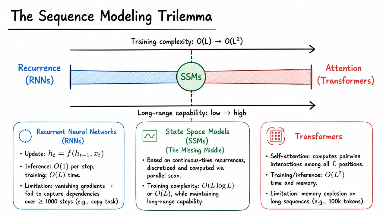
1. The Sequence Modeling Trilemma
Sequence modeling stands at the center of many of today’s most compelling AI applications—from language generation to audio understanding and time-series forecasting. At first glance, these tasks share a common structure: we observe a stream of data and we need to map it to a stream of predictions or representations, one per step. But beneath this simple framing lies a deep architectural tension. Every practical sequence model must navigate a trilemma: it must be efficient to train, it must capture dependencies that span thousands of steps, and it must adapt to the varying needs of different modalities and lengths. No single architecture has perfectly solved all three desiderata, and understanding why illuminates why state space models (SSMs) have emerged as such a promising middle path.
The two classic extremes of this trilemma are recurrent neural networks (RNNs) and Transformers. An RNN maintains a fixed-size hidden state and updates it with each new input via a recurrence:
During training, the forward pass progresses step by step, giving total time ; at inference the cost per token is a constant . This linear complexity makes RNNs attractive for long streams. However, the very mechanism that yields efficiency—a compressed state that summarizes all past inputs—is also its Achilles’ heel. Gradients must flow backward through time along the same recurrence, and over long horizons they tend to either explode or, more commonly, vanish. In practice, a vanilla RNN struggles to remember information beyond a few hundred steps. The classic copy task shows this dramatically: when asked to reproduce a token seen 1000 steps ago, the RNN fails because the signal has been diluted out of the hidden state.
Transformers tackle the long-range weakness head-on by removing the fixed-size state. A Transformer uses self-attention to compute pairwise interactions between all positions in the sequence. This gives the model direct access to any past token, and gradients flow through a fully connected graph rather than a chain. The result is the ability to model extremely long-range dependencies, as evidenced by in-context learning in large language models. The price is computational: training and inference both require time and memory because every query attends to every key. On sequences of 100k tokens or more, this quadratic cost explodes, making Transformers infeasible without aggressive approximation tricks or model parallelism.
These two extremes paint a clear picture of the trilemma. RNNs are efficient but short-sighted; Transformers are long-range masters but quadratically expensive. For many real-world tasks, we crave a model that can see far into the past while remaining sub-quadratic at training time. State space models (SSMs) are designed to inhabit that missing middle. They borrow the stateful recurrence idea from RNNs but give it a richer, mathematically grounded parameterization inspired by continuous-time dynamical systems. Crucially, the SSM recurrence is structured so that it can be computed in parallel using prefix-sum algorithms like the associative scan. This lifts training complexity to or even while still maintaining much stronger long-range modeling capabilities than a vanilla RNN. The result is a sequence model that sits between pure recurrence and full attention in both compute cost and representational power, offering a desirable compromise.
A compact way to internalize this landscape is through a one-dimensional spectrum that orders architectures by their training cost and long-range capability. The visual below—often labeled The Sequence Modeling Trilemma—depicts exactly that. A horizontal bar marks the architectural spectrum: the left endpoint corresponds to pure recurrence (RNNs), with a soft blue shade to evoke simplicity and low cost; the right endpoint represents full attention (Transformers), rendered in red to highlight quadratic expense. Exactly at the midpoint, a prominent green marker identifies state space models. Above the bar, a left-to-right arrow captures the rise of training complexity from to ; below the bar, a second arrow traces long-range capability from low to high. A dashed vertical line through the SSM marker emphasizes that this is not merely a midpoint of compromise but a sweet spot where sub-quadratic time meets sufficient long-range reach.
This diagram consolidates the earlier arguments into a single glance. The trade-off becomes tangible: moving right improves long-range modeling at the cost of quadratic scaling, while moving left sacrifices memory for speed. SSMs, by leveraging parallel scans and continuous-time discretization, stake out a region that gives practitioners the best of both worlds—efficient training and the ability to capture dependencies that would leave a plain RNN blind. As we dive into the technical machinery behind Mamba‑3, keep this spectrum in mind; every design choice will be a step along this axis, carefully tuned to widen the middle ground.
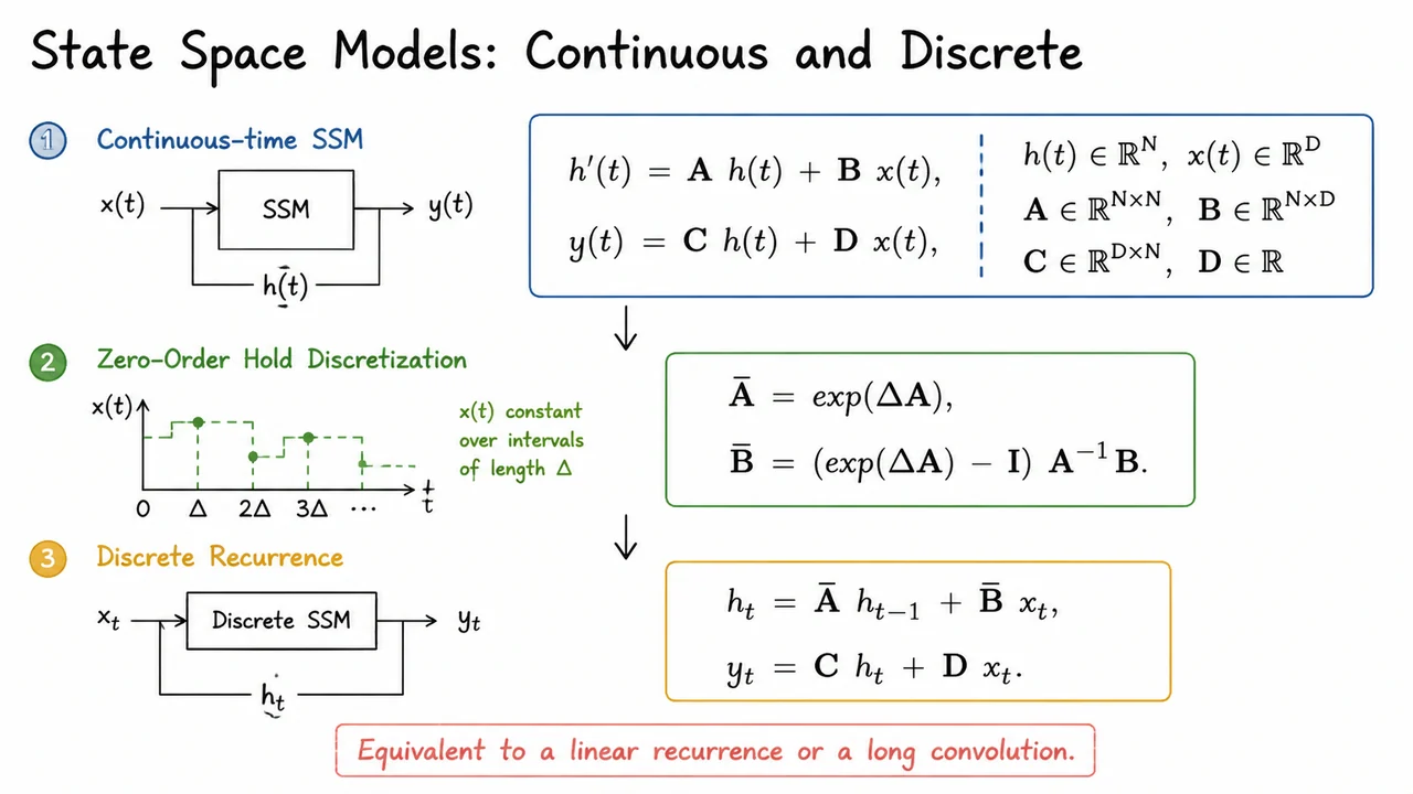
2. State Space Models: Continuous and Discrete
Having framed the sequence modeling trilemma—that a single architecture cannot simultaneously achieve constant memory, parallelizable training, and unbounded context without tradeoffs—we now turn to the class of models that has quietly sidestepped this dilemma: state space models (SSMs). The foundational idea is to borrow from control theory and describe sequence transformations as a dynamical system that evolves a continuous hidden state over time. This perspective unifies recurrence and convolution, and the jump from continuous to discrete time is the crucial step that makes SSMs practical for deep learning. In this section, we walk through the continuous-time definition, its discretization via a zero-order hold (ZOH), and the resulting linear recurrence—the backbone of every model from S4 to Mamba-3.
A continuous-time state space model is governed by a pair of equations: a differential equation for the hidden state and a linear observation equation. Formally, for an input signal and hidden state , the system is where is the state transition matrix, the input projection, the output projection, and the scalar (often omitted or set to zero) a direct feedthrough. The first equation tells us how the internal state changes in response to the current input, while the second produces a continuous output as a linear readout of that state. The state dimension controls the model’s capacity to memorize and mix information over time, analogous to the number of hidden units in an RNN. What makes this formulation powerful is that it decouples the dynamics (the pair) from the readout (), permitting independent design of memory mechanisms and output mappings.
The continuous-time system is elegant but not directly computable on discrete sequence data. We receive samples at discrete time steps, and we need to produce corresponding outputs . The bridge is discretization: we assume a constant step size (which can be learned or fixed) and approximate the input as piecewise constant over each interval . This assumption, known as a zero-order hold, yields explicit formulas for the discrete parameters and : Here denotes the matrix exponential. The first equation says that the state evolves without input according to the matrix exponential of scaled by ; the second integrates the input over the interval, accounting for the state evolution it induces. If is not invertible, the formula for requires a generalized inverse, but in practice structured matrices (e.g., diagonal or HiPPO) avoid this issue. The crucial takeaway: discretization compresses the continuous dynamics into a pair of discrete matrices that exactly match the ZOH assumption.
Once and are fixed, the continuous system reduces to a simple linear recurrence over the discrete time steps: Here is the vector input at step , is typically initialised to zero, and is the output. This recurrence is exactly the update rule of a linear RNN—but with a critical difference: the recurrence weights are not learned directly; they are derived from continuous parameters and the step size . The state now encodes a compressed history of all previous inputs, with the forgetting and mixing patterns determined by the eigenvalues of . Because is obtained via a matrix exponential, we can design continuous to have specific properties (stability, long-range memory) and know they will be faithfully transferred to the discrete domain.
The equivalence between the discrete recurrence and a long convolution opens up a second computational pathway. Unrolling the recurrence: and since , the output becomes a convolution of the input sequence with a kernel (plus the skip connection ). During training, this kernel can be computed for all time steps in parallel using fast Fourier transforms (FFTs), making SSMs highly efficient on modern hardware. This duality between recurrence and convolution is what initially allowed SSMs to resolve the sequence modeling trilemma: constant state size for inference, parallel convolutions for training, and, with appropriate parameterizations, arbitrarily long-range memory. The price? The kernel is fixed by the SSM parameters, so the model cannot selectively attend to different inputs—a limitation that would later motivate selectivity in Mamba.
The visual below captures this three-stage transformation in a clean, diagrammatic form. At the top, the continuous-time ODEs— and —define the abstract dynamics. The middle block shows the discretization step: the continuous matrices are turned into discrete via the matrix exponential and the ZOH integral, with explicitly present. Finally, the bottom block displays the discrete recurrence , , with a note that this is equivalent to a linear recurrence or a long convolution. The visual hierarchy reinforces the conceptual flow from continuous theory to practical computation, using minimal text and a subdued color palette to keep the equations at the forefront. It is a succinct reminder that SSMs are defined by ODEs, made tractable through discretization, and deployed as either recurrent or convolutional operators.
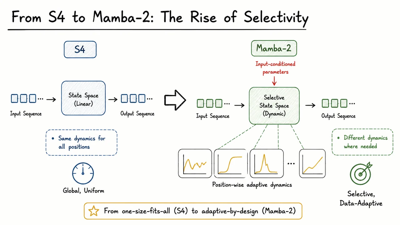
3. From S4 to Mamba-2: The Rise of Selectivity
The elegant machinery of continuous-time state space models, discretized via zero-order hold, forms the theoretical backbone of deep SSMs. In the previous section, we saw how a linear time-invariant (LTI) system with parameters can capture a recurrent state update, and how discretization turns it into a sequence transformation that is both recurrent and convolutional. S4 built on this foundation by carefully structuring the state matrix —using HiPPO-derived matrices and diagonalization—to achieve stable long-range memory while remaining computationally efficient through a parallel convolution mode. Yet for all its cleverness, S4 carries a fundamental limitation: its dynamics are time-invariant. The same matrices process every token in a sequence, regardless of what that token actually means. In language modeling, where the word “bank” drastically changes meaning depending on whether the nearby context speaks of rivers or finance, this fixed-state lens is a heavy blindfold.
The need to break away from time invariance gave birth to selectivity—the idea that the model’s own hidden state update should depend on the content it is reading. This isn’t just a convenience; it is a requirement for any model that hopes to learn contextual pattern-matching or to implement what is sometimes called “selective attention” across time. Once we admit that the state transition itself must be data-dependent, the LTI paradigm collapses. The convolution trick for fast training no longer applies because and now vary per time step, and the system becomes a time-varying state space model. Mamba, introduced as an SSM with S6 (Selective Scan), is exactly that: and (and the discretization step size ) are generated from the input at each time step via simple linear projections. The resulting recurrence is still a structured state update, but it can no longer be unrolled into a single global convolution. Instead, Mamba computes the sequence using a hardware‑aware parallel scan, which treats the linear recurrence as an associative operation—like a parallel prefix sum—adapting it to modern GPUs by exploiting memory hierarchy and recomputation to keep the workload efficient.
Mamba-2 takes this evolution one crucial step further. While S6 solved the expressivity problem, its parallel scan was less efficient than the pure convolution of S4 for certain hardware operations, especially on tensor cores. Mamba-2 reformulates the state space model so that the time-varying state update corresponds to a structured matrix that is semi‑separable. This algebraic insight means that the entire sequence transformation can be decomposed into a combination of parallel scans and structured matrix multiplications that map perfectly onto tensor core‑optimized primitives. The parameterization remains input-dependent: and the parameters are still functions of the token, keeping selectivity intact. But by reorganizing the computation into a form where the SSM is expressed as a matrix that is both diagonal-plus-low-rank and semi‑separable, Mamba-2 achieves a training speed that rivals or surpasses the convolution mode while preserving the adaptive power of selective recurrences.
Understanding this lineage requires holding three competing desires in view: long-range memory, input‑aware selection, and hardware‑optimal parallelism. S4 gave us the first, Mamba introduced the second, and Mamba-2 reconciles all three. The visual summary below makes that arc instantly readable. It sketches a timeline from a fixed‑parameter SSM with a global convolution to a selective SSM with a parallel scan, and finally to the Mamba-2 formulation that frames the selective recurrence as a structured matrix multiplication suitable for tensor cores. The diagram uses clean, hand‑drawn arrows and sparse labels to emphasize the core shift: from static to dynamic state matrices, and from a single computational strategy to a hybrid design that respects both model expressivity and hardware reality. Seeing the three stages side by side drives home why each step was necessary—and why Mamba-3 can now build on a foundation where selectivity is no longer a luxury but a solved primitive, ready to be composed with other architectural innovations.
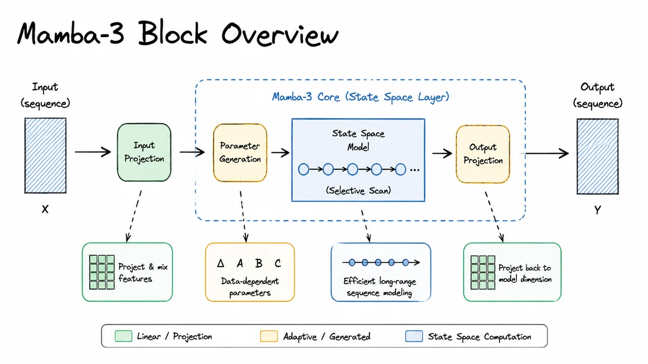
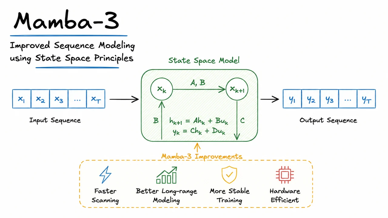
4. Mamba-3 Block Overview
Having seen how selectivity empowers state-space models to adapt their dynamics to input content, we now turn to the architectural blueprint that packages this idea into a practical, high-performance neural network block: the Mamba-3 block. Where earlier designs either sacrificed parallelism for selectivity (Mamba’s sequential recurrence) or relied on fixed linear recurrences to achieve efficient training (S4), Mamba-3 strikes a balance by marrying input‑dependent selectivity with a parallel associative scan. The result is a single block that can be stacked like a Transformer layer, processes entire sequences in sub‑quadratic time, and retains the nuanced adaptive behavior that made selective SSMs so compelling.
At its core, the Mamba-3 block implements a linear time‑varying state‑space model whose parameters , , and are small learned functions of the input . For a sequence of length with feature dimension , the block first expands the input via a linear projection to an internal dimension (usually or a small multiple), from which it computes:
- A delta vector that controls the discretization step size and hence the timescale of the dynamics,
- An input matrix (often represented as a vector broadcast over a state dimension),
- An output matrix ,
- And an optional residual skip connection that will later be gated.
The continuous‑time state matrix is typically chosen as a fixed diagonal matrix with learnable eigenvalues, e.g., . Its constancy and diagonal structure are essential for both modeling long‑range dependencies and enabling efficient parallel scans.
Discretization via a zero‑order hold (ZOH) turns the continuous ODE into a recurrence that respects the variable sampling intervals. With step size , the discrete matrices become
or, in a more numerically stable form for the diagonal case, simply and
computed elementwise with the corresponding ZOH formula. This yields a linear recurrence
where is the scalar input at time (computed from the projected input) and is the hidden state. Crucially, the recurrence is linear in the state, even though the parameters depend nonlinearly on the input. This linearity in the state dimension is what allows us to replace the slow sequential loop with a parallel scan.
Because any linear recurrence of the form can be seen as a prefix sum over a suitable monoid, we can compute all hidden states simultaneously using a parallel associative scan. The monoid elements are pairs with a binary operation that mimics composition of affine maps. The parallel scan yields complexity (or even with work‑efficient algorithms) while running entirely on parallel hardware, in stark contrast to the sequential steps of the original Mamba block. This is the key architectural innovation that makes Mamba-3 block competitive with attention‑based models for fast training.
Completing the block, the scalar outputs are collected into a sequence and then modulated by a gating mechanism that closely resembles a gated linear unit (GLU). Unlike the plain SSM output, the block passes the original input projection through a nonlinearity (e.g., SiLU) and multiplies elementwise by the SSM output. This gate acts as a data‑controlled skip connection, allowing the network to decide at each position how much of the state‑space pathway to use versus the direct input contribution. A final linear projection and a residual connection wrap the block, with layer normalization (typically RMSNorm) applied before the core computation for training stability.
Stepping back, the Mamba-3 block can be mentally decomposed into three sequential stages:
- Parameter projection: input → (and the gating branch).
- Selective SSM: discretization + parallel scan → hidden states → .
- Gating and residual: output gate, projection, and skip connection.
The visual below captures this entire chain in a compact diagram. Input enters on the left, splits into the parameter branch and the gating branch. The parameter branch produces ; these flow through a “Discretize” operation that yields . The parallel scan block, drawn as a central computational unit, receives the discretized coefficients and the input signal and efficiently computes the output sequence . A multiplicative gate combines the SSM output with a nonlinear transform of the input, and a residual addition completes the block. The hand‑drawn aesthetic and arrow connectors reinforce the modular, sequential flow while keeping attention on the three major innovations: input‑dependent discretization, parallel linear recurrence, and gated output. After absorbing the full picture, we are ready to delve into the precise mathematical derivation of the zero‑order hold discretization that makes the selective SSM possible.
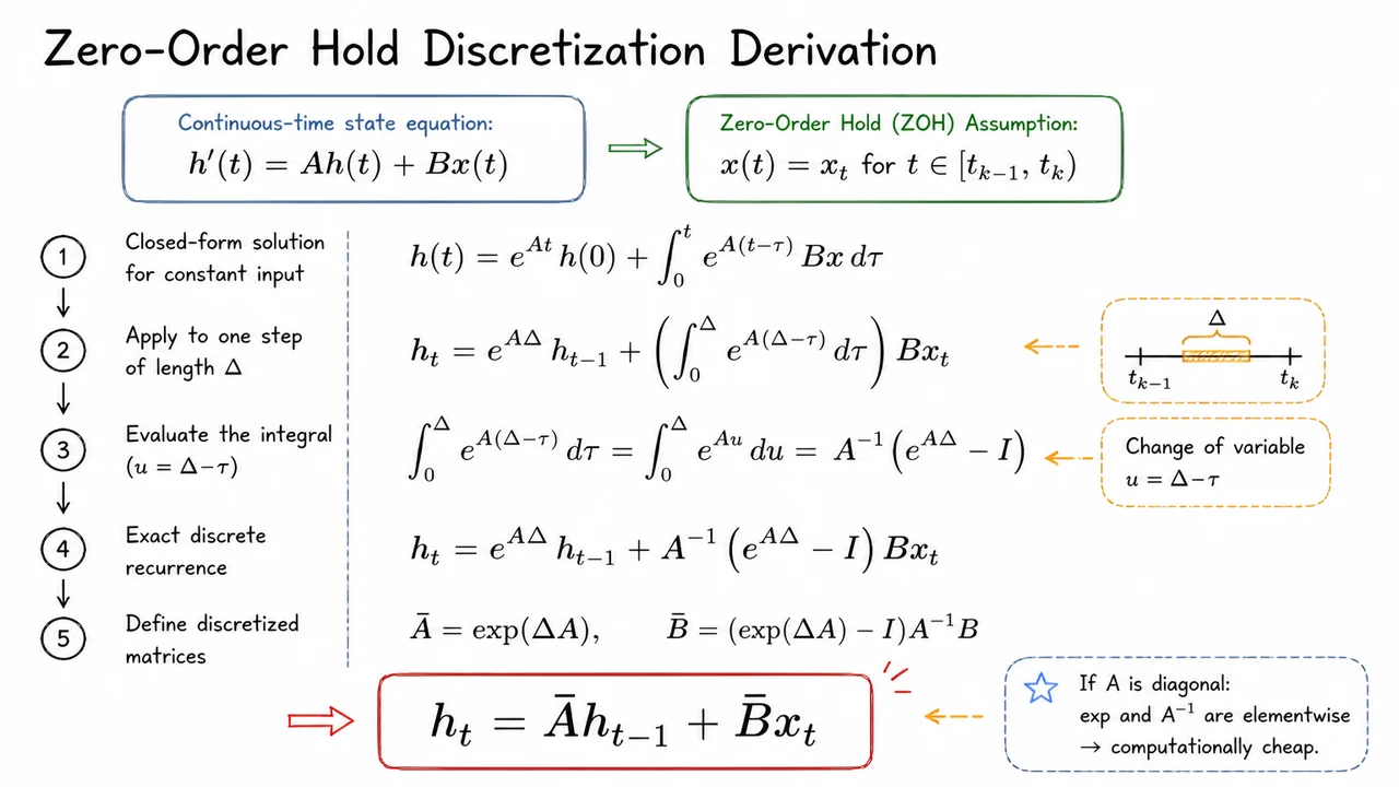
5. Zero-Order Hold Discretization Derivation
Having seen how the Mamba‑3 block weaves together a state‑space core with a selection mechanism, we now turn to the quiet but essential bridge that turns a continuous‑time differential equation into a discrete sequence transformation we can actually compute. The continuous state‑space model describes a smooth evolution:
where is a latent state, an input signal, and are matrices (or, in Mamba, structured diagonal matrices). To process a sequence of discrete tokens , we must choose a discretisation rule that produces a recurrence . The zero‑order hold (ZOH) assumption is the simplest consistent choice and, remarkably, yields an exact discrete recurrence with no approximation error for the given input sampling scheme.
The ZOH assumption says: over each discrete interval of length , the input is held constant at the value sampled at the start, i.e. for . This is natural when the input is itself a sequence of scalars or vectors coming from a tokeniser—there is no finer‑grained signal between the samples. Under ZOH, the ODE becomes a linear system with constant coefficients on each step, and its solution can be written in closed form using the matrix exponential.
Consider a single interval. If we set and treat constant, the state at any time is given by the familiar variation‑of‑constants formula:
Plugging in the constant input and evaluating at the end of the interval , we get the discrete state update:
The integral of the matrix exponential appears messy, but a simple change of variable turns it into the fundamental matrix integral . If is invertible, this integral has the closed form
The invertibility condition is not a problem in practice. Mamba‑3 uses a diagonal whose entries are negative to ensure stability, so the diagonal elements are never exactly zero and the inverse exists element‑wise (if needed, the formula can be extended via limits). For a diagonal , the matrix exponential and inverse reduce to simple, independent scalar operations on each channel, making the whole discretisation computationally trivial.
Now the exact discrete recurrence emerges clearly. Define the discretised matrices
and the state update collapses to the elegant, linear recurrence
This is the same structural form that runs through the entire Mamba family: a simple state‑space recurrence whose dependence on the time step is baked into and via the matrix exponential. The real power, as we will see, is that this recurrence can be computed in parallel for all time steps using associative scan algorithms, provided that is a structured (in particular, diagonal) matrix.
The visual below organises this derivation from top to bottom. It begins with the original continuous ODE in a quiet reference box, then steps through the ZOH assumption and the closed‑form solution, the integral evaluation, and finally the definition of and . The terminal, boxed recurrence stands out as the takeaway, while a small handwritten note reminds us that for diagonal everything becomes element‑wise and extremely cheap—an echo of the computational efficiency that makes Mamba‑3 practical for very long sequences. The entire flow reinforces that discretisation is not an approximation but an exact algebraic consequence of holding the input constant, and that the resulting linear recurrence is the perfect launchpad for the parallel scan that follows.
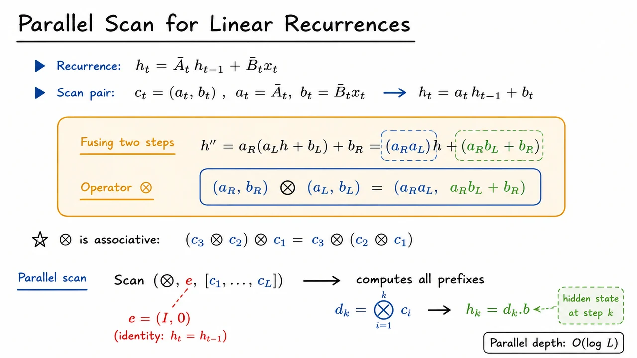
6. Parallel Scan for Linear Recurrences
After the zero-order hold discretization, we possess a clean linear recurrence that describes the evolution of the hidden state at each timestep:
The parameters and are now input‑dependent (the selective mechanism), so they can vary across the sequence. Naively, computing all requires a strictly sequential loop over the time steps, because each needs . For long sequences this sequential bottleneck becomes a serious obstacle, especially on GPU‑style hardware that thrives on parallelism. The breakthrough of Mamba‑3 is to recognise that this particular recurrence can be restructured into an associative prefix problem, whose depth can be compressed from to by using parallel scans.
The central trick is to pack each time step’s contribution into a small pair that behaves like an affine transformation. Notice that the update rule can be read as: start with , multiply by , then add . We therefore define a scan pair for step :
Now the recurrence becomes . Viewed abstractly, each pair is a tiny machine that consumes a hidden state and outputs a new one. The insight is that we can combine two such machines into a single equivalent machine by chaining them.
Consider two consecutive steps: first we apply the left step to some initial state , giving (h
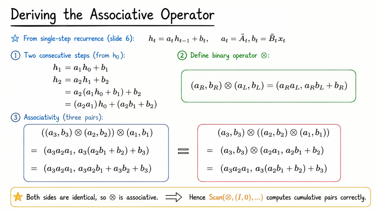
7. Deriving the Associative Operator
With the parallel scan scheme from the previous section in hand, the next step is to define the right composition operator that can fuse consecutive linear recurrence steps into a single, equivalent step. This operator will become the core of the scan routine, allowing us to compute all hidden states in depth instead of the naive sequential .
Recall the single-step recurrence that lies at the heart of Mamba‑3’s selective state‑space dynamics:
Here is the hidden state at time , is a scalar (or diagonal matrix) that controls how much of the previous state is retained, and is the new input contribution, itself a product of the input-dependent and the input token . For the recurrence to be amenable to parallel prefix‑sum techniques, we need to understand what happens when we move forward by more than one step.
Consider two successive steps from the same initial state . Expanding directly, This one‑line calculation reveals the structure of a composite transformation: the combined effect of the two steps is again an affine map of the original state, with a new multiplicative factor and a new additive bias . In other words, the pair followed by can be collapsed into a single pair .
This observation immediately suggests a binary operator that takes the right pair (the later step) and the left pair (the earlier step) and produces their composition: Here the order matters: the left operand corresponds to the transformation that is applied first, and the right operand to the one applied second, exactly as we dress the equations from the inside out. Notice that this operator is not commutative—applying the steps in reverse order would give a different result—but commutativity is not required for a parallel scan; we only need associativity so that the combining order does not matter.
Checking associativity is straightforward algebraically. Take three arbitrary pairs . Grouping from the left first: Grouping from the right instead: Both evaluation orders yield exactly the same composed pair, so is indeed associative. Moreover, the identity element for this operator is the pair (where for scalar or the identity matrix in the general case), because applying it before or after any step leaves the transformation unchanged. This identity is exactly the initial value we will feed into the parallel scan.
The associativity of is the linchpin that allows us to compute all cumulative pairs in parallel using a binary tree reduction. Instead of scanning left‑to‑right, we can combine adjacent segments in any order that respects the tree structure, and the final results—the cumulative pairs up to each index—will be identical to the sequential composition. This is why the parallel scan can safely replace the naive recurrence in Mamba‑3 without introducing any numerical discrepancy.
The visual below distills this derivation into a compact reference. Titled “Deriving the Associative Operator”, it displays the single‑step recurrence, the two‑step expansion that motivates the composition rule, the boxed definition of , and two parallel columns confirming associativity with the three‑step case. The hand‑drawn style and sparse layout make the logical flow instantly clear: the operator emerges naturally from the affine structure of the recurrence, and the equality of both groupings proves we can trust the parallel scan to behave exactly like a sequential pass.
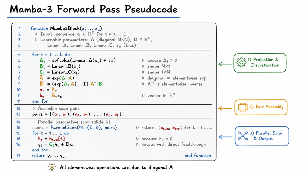
8. Mamba-3 Forward Pass Pseudocode
Having established the associative operator that fuses two state-space segments into one, we can now confront the central computational challenge of Mamba-3: how to evaluate a linear recurrence whose transition matrices and input projections depend on each token in the sequence. In a standard time-invariant SSM, the same and apply everywhere, so we can unroll the recurrence into a convolution with a fixed kernel computed once. But Mamba-3 makes , , and functions of the input . That means the recurrence is no longer a convolution; it is a selective scan through a sequence of varying linear dynamics. The naive sequential loop over is fast for inference but paralyzes training because it cannot be parallelized. The solution, as hinted in the previous section, is to reorganize the recurrence as a prefix-sum problem over an appropriate semigroup and then apply a parallel associative scan.
The forward pass of a Mamba-3 block therefore becomes a carefully choreographed pipeline: project the token into the control signals, discretize the continuous-time parameters to obtain per-token and , package those into scan-compatible pairs , run the parallel scan to recover all hidden states, and finally project back to the output space. Let’s walk through each phase.
For every token , three linear projections produce the raw ingredients. First, the time-step pre-activation is passed through a softplus to give , ensuring that the discrete-time system remains stable and causal. Second, yields a vector , and gives a row vector . The state size is usually much smaller than the input dimension , so these projections are cheap.
The continuous-time state matrix is a fixed learnable diagonal matrix . Thanks to diagonality, all operations on reduce to elementwise operations on its diagonal entries. This is critical: it makes the matrix exponential, matrix inverse, and logarithms trivial. The discretization follows the zero-order hold (ZOH) rule, giving Because is diagonal, is simply elementwise exponentiation of the diagonal scaled by , and is elementwise reciprocal. The resulting remains diagonal, and is a vector.
Now, recall the discrete-time state recurrence: with . This is not yet in the form of a binary associative operation. However, we can rewrite each step as a transformation on a pair that carries the cumulative effect of previous states. Define Then the recurrence becomes We can view this as applying a linear function to the initial state. If we define an operator that composes two consecutive steps, then the cumulative effect from time 1 to is the scan result and the hidden state is exactly . The identity element for this operator is , matching the base case . This is exactly the prefix-sum we derived in the previous section, now populated with per-token data.
The parallel scan operator (also called the Blelloch scan for associative operations) can then compute all cumulative pairs in work and span when using processors in parallel. In practice, on GPU implementations, the work is split across threads in a highly optimized fashion. Once we have all , the output is simply where is a learnable skip connection (often a diagonal matrix that is easily applied elementwise). This skip connection ensures that even if the state space path fails to capture certain aspects, the raw input can flow through.
The pseudocode on this slide distills these steps into a clean algorithmic block. A large code box with three conceptual compartments mirrors the natural phases of the computation: (I) per-token projection and discretization, (II) assembly of scan pairs , and (III) the parallel scan call followed by the output projection. The scan line is visually emphasized because it is the workhorse that makes the selective recurrence feasible for training. Beneath the box, a subtle note reminds us that all matrix operations on are elementwise due to its diagonal structure, which is the hidden key that keeps the cost linear in instead of quadratic. The visual thus serves not as a verbatim copy of the lecture notes but as a compact, glanceable summary of the three-step recipe that turns a deeply sequential problem into one suited for modern parallel hardware.
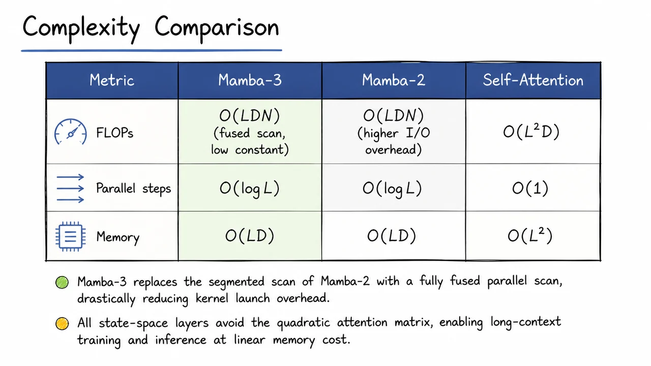
9. Complexity Comparison
After walking through the forward pass of Mamba‑3—where a parallel associative scan fuses the linear recurrence and the selective gating into one efficient kernel—the natural next question is: what does this buy us in practice? Elegant pseudocode only matters if it translates into concrete computational advantages. To answer that, we need to compare the per‑layer resource requirements of Mamba‑3 against its immediate predecessor Mamba‑2 and the ubiquitous self‑attention baseline. The numbers that emerge reveal why Mamba‑3 stands as a genuinely practical architecture for sequences whose length can stretch into the hundreds of thousands.
Let’s set the stage. We have a sequence of tokens of length processed by a layer of width (the model dimension). In self‑attention, each token interacts with every other token via an attention matrix, whose computation famously consumes floating‑point operations (FLOPs) and demands memory for the attention logits or the softmax matrix. This quadratic growth makes long‑context training and inference prohibitively expensive. State‑space models (SSMs) avoid the explicit matrix entirely by maintaining a small recurrent state of size (the state dimension) and updating it token‑by‑token via a linear recurrence. The recurrence can be unrolled into a parallel scan over steps, where each step combines two or operations. The total FLOPs for a layer are therefore —linear in both sequence length and model dimension, with an extra factor of that reflects the state size. Because is typically small (often 16–64), this remains far more efficient than the quadratic self‑attention alternative.
But the asymptotic cost does not tell the whole story. The constant factors and hardware utilisation determine whether a model can train at scale with reasonable throughput. That is where the difference between Mamba‑2 and Mamba‑3 becomes critical. Mamba‑2 implemented a segmented scan: it split the sequence into chunks, performed independent scans within each chunk, and then combined the partial results with a second pass. This algorithm kept the parallel depth (the number of sequential steps in the critical path) at , but it introduced multiple kernel launches and data‑transfer points between the chunk‑wise scans and the final reduction. The resulting I/O overhead inflated the constant in front of and led to under‑utilisation of the GPU’s compute units.
Mamba‑3 replaces this segmented approach with a fully fused parallel scan. The entire recurrence is carried out in one kernel that uses the same parallel tree‑reduction structure but streams data only once through the GPU’s memory hierarchy. Kernel‑launch latency vanishes; intermediate results stay in on‑chip memory (shared memory or registers). The upshot is a dramatically lower constant factor on the same FLOP count, giving better hardware utilisation and faster wall‑clock training times than Mamba‑2, even though both share the same asymptotic complexity class.
Another axis to compare is the parallel depth of the layer. Self‑attention, once the matrix is computed, can (in theory) perform the softmax and the value mixing in a fully data‑parallel way, leading to a parallel depth of —a constant independent of . In practice, the quadratic memory and the cost of materializing the attention matrix often force block‑wise or sharded implementations that degrade this ideal. State‑space layers, in contrast, must always perform a scan, whose inherent dependency chain gives a parallel depth of . Both Mamba‑2 and Mamba‑3 exhibit this logarithmic depth; the difference is that Mamba‑3’s fused scan executes those logarithmic steps without ever writing intermediate buffers to global memory, so the depth penalty is far less painful than it might seem.
Finally, memory consumption is a decisive factor for scaling to long contexts. Self‑attention’s memory footprint (intermediate activations for backpropagation) severely limits the feasible sequence length during training. Both Mamba‑2 and Mamba‑3 reduce this to —the memory required to store the input and output activations and the relatively tiny state buffers—because the scan directly computes the output without ever materialising an matrix. This linear memory profile is the primary reason state‑space models can train on sequences with lengths exceeding one million tokens on a single GPU.
The visual below consolidates these per‑layer computational characteristics into a clean, at‑a‑glance comparison. It shows the three architectures side‑by‑side across the key metrics of FLOPs, parallel steps, and memory. In the FLOPs row, both Mamba variants share the entry, but a note distinguishes Mamba‑3’s fused scan with its low constant from Mamba‑2’s higher I/O overhead. The parallel‑steps row reminds us that both SSM layers are logarithmic in while self‑attention remains constant. The memory row starkly contrasts the footprint of the SSMs with the explosion of attention. Together with the accompanying bullet points—highlighting the fused scan and the avoidance of the quadratic attention matrix—this table makes it immediately obvious why Mamba‑3 is not just another incremental tweak but a genuine step forward in making long‑context sequence modeling practical.
10. Correctness of the Parallel Scan Recurrence
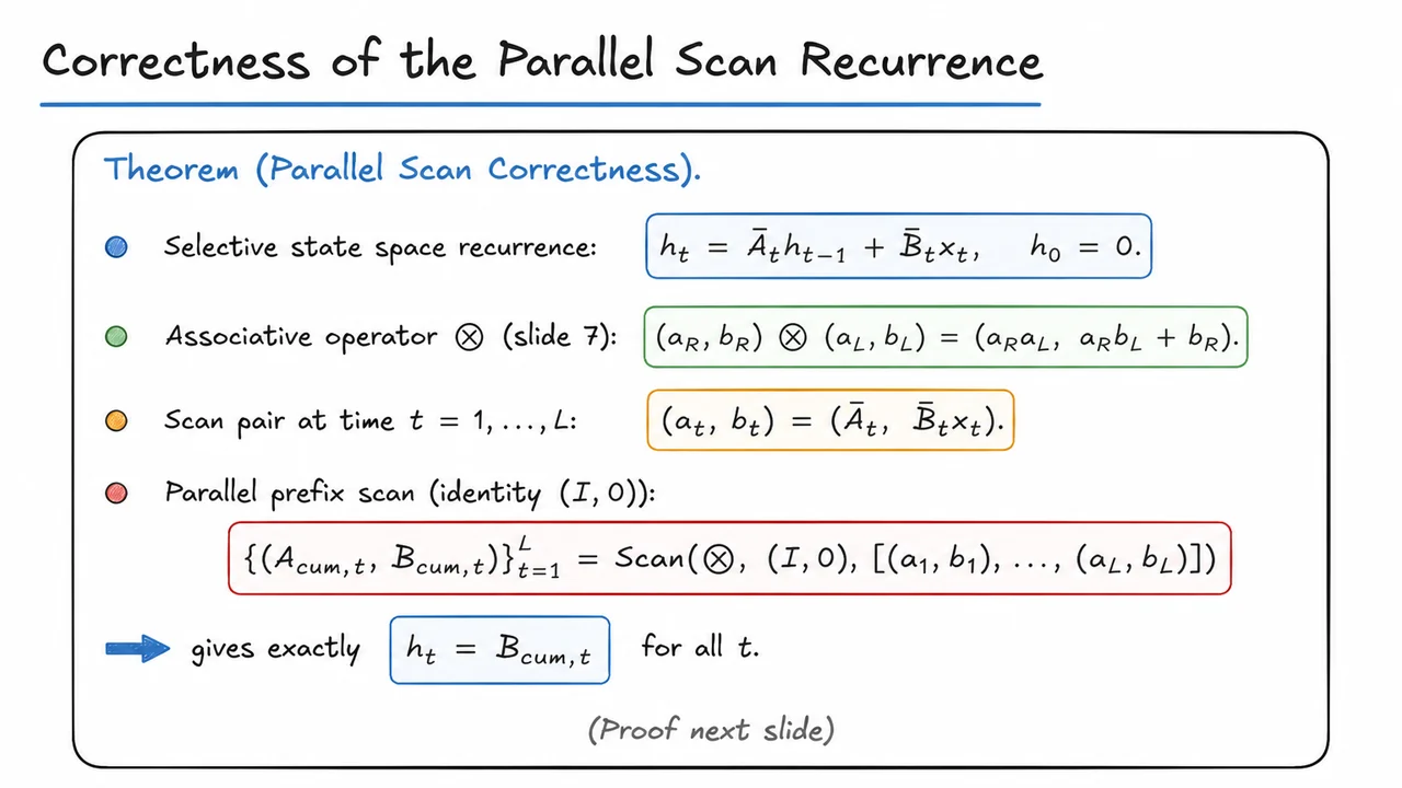
Earlier we analyzed the asymptotic complexity of Mamba-2 and saw how the parallel associative scan can turn an apparently sequential bottleneck into a sub‑quadratic computation. But that promise depends on a subtle property: the parallel scan must compute exactly the same hidden states that would be produced by the recursive formula, step by step. The correctness theorem connects the dots—it shows that by packaging the state‑space parameters into a specific pair and applying a well‑designed associative operator, the prefix scan precisely reproduces the selective recurrence, with no approximation.
Let’s start from the recurrence itself. In Mamba‑3 the hidden state evolves as
Here and come from the discretization of a continuous‑time SSM and can depend on the input ; that’s the selective mechanism. Because each step depends on the previous hidden state, a naïve implementation loops over and is inherently sequential—it runs in time with parallel depth. The parallel scan, by contrast, promises depth if we can reframe the computation as a binary associative operation over a list of elements.
The key is to view each time step as an affine map on the hidden state. For a given , the transformation is
We can encode this map compactly by the pair
thinking of it as “multiply the incoming state by , then add .” When we compose two such maps—say first apply the earlier step’s transformation and then the later step’s transformation —the resulting map is again affine:
This composition suggests a binary operator defined by
If the operator is associative, then we can compute the cumulative effect of any prefix of steps by repeatedly applying to the corresponding list of pairs; the order of combining groups of steps does not affect the final result.
Now consider the full sequence of time steps. For each we have the pair . The parallel prefix scan takes the list and, using the associative operator together with the identity element (representing “do nothing” to the hidden state), produces cumulative pairs
The cumulative pair encodes the affine map that sends the initial hidden state all the way to :
Because we chose , the term vanishes, leaving simply
Thus the recurrence’s hidden states are recovered exactly as the second component of the prefix‑scan output. The associative property (proved on the next slide) guarantees that this holds regardless of how the scan is parallelised—whether via a tree reduction, a Blelloch scan, or a work‑efficient algorithm—as long as the operator is applied correctly.
In Mamba‑3, is a diagonal matrix (often scalar per channel), and is a vector; the operator applies elementwise across all channels, so the scan can be performed independently for each dimension of the hidden state. This mapping from a selective state‑space model to a parallel prefix scan is what unlocks sub‑quadratic training: we can compute all with work and parallel depth, while the scan outputs remain identical to the sequential recurrence.
The visual below consolidates the theorem succinctly. It lists the original recurrence, the definition of the associative operator, the construction of the scan pairs, and the scan call with the identity element. The final emphasised line——is the punchline: the parallel scan, when instantiated with these correctly built pairs, yields the exact hidden states of the selective SSM. That visual serves as a one‑glance reference, distilling the logical chain from discretisation to parallel computation and setting the stage for the inductive proof that follows.
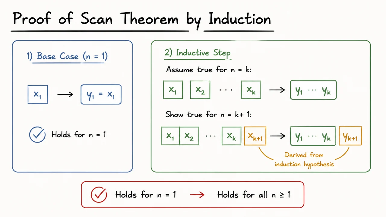
11. Proof of Scan Theorem by Induction
After establishing that the parallel scan recurrence is correct, we need to know why it works—and that answer comes from the Scan Theorem, proved by induction. In the Mamba-3 architecture, the core computation is a linear recurrence:
where is the hidden state, is a diagonal state transition matrix (or a scalar per channel), is the input projection, and is the input at time . This recurrence looks sequential: you must compute , then , and so on. Yet to unlock efficient parallel training and hardware utilization, Mamba-3 casts this recurrence as an associative scan—a prefix sum over a special semigroup where the “sum” operation corresponds to composing linear updates. The magic that guarantees the scan yields exactly the correct for every is the Scan Theorem, whose proof is a simple but illuminating induction.
To see the connection, define a 2‑tuple and a binary operator that combines two consecutive segments. For two contiguous intervals, the combined effect is
where the operation captures the matrix multiplication and addition:
Why this particular form? If we have entering the first segment, then the state after the first segment is , and after the second segment, . So the pair correctly represents the cumulative effect of both segments on an initial state. This composition is associative: you can group segments in any order, and the final pair will correctly compute the state after the combined interval. An associative scan over the sequence with initial state (or a learned initial value) then produces the sequence of pairs , from which we extract the second component to obtain for all .
The Scan Theorem states that a divide‑and‑conquer algorithm based on this associative operator is correct: if we split the sequence in half, recursively compute the cumulative pair for each half, and then combine the results using , the output matches the sequential definition. More precisely, for any associative operator on a set , the parallel prefix algorithm (scan) applied to a sequence yields the same result as the sequential left‑fold, provided the algorithm respects the operator’s associativity. The theorem is proved by induction on the length of the sequence.
Let’s sketch the induction. Base case: , the scan of a single element is the element itself, trivially the correct cumulative value. Inductive step: assume the parallel scan works correctly for all sequences of length strictly less than . For a sequence of length , the algorithm partitions the input into two halves of lengths and . It first computes the cumulative pairs for each half independently (by the induction hypothesis, these are correct fold‑sums over the respective sub‑sequences). Then it propagates the final cumulative pair of the left half to each element of the right half by applying the operator between that left‑half total and the right‑half element’s own cumulative. Formally, if the left half total is , then for every element in the right half with local cumulative , the final cumulative becomes . Because is associative, this exactly matches the sequential fold that would combine with the right‑half elements. No global order is violated: the parallel structure merely regroups the associative operations, and associativity guarantees the outcome is the same. The induction closes, proving the algorithm’s correctness for all .
Why does this matter for Mamba‑3? The parallel scan is what converts an ostensibly sequential recurrence into a form that can be computed with depth on parallel hardware. The induction proof confirms that the intermediate combinations, no matter how they are scheduled (e.g., using a tree reduction), preserve the exact sequence of state updates. Without this guarantee, any speedup would be suspect. In Mamba‑3, the operator is not a fixed matrix multiplication; the transitions and depend on the input, making the scan selective. The Scan Theorem still holds because the operator remains associative even when its components are dynamic—the proof only relies on the algebraic property of , not on its parameters being constant. This foundational result is thus the linchpin that enables Mamba‑3 to fuse selective state updates with efficient parallel computation.
The visual that follows encapsulates the proof’s two phases: the induction base case (a single element scan) and the inductive step that stitches together two halves using the associativity of . In the diagram, you’ll see a tree‑like structure where a left‑pointing arrow carries the total of the left half to combine with each right‑half element, while circular nodes represent the associative operator. The labels “Base Case” and “Inductive Step” anchor the logical flow, and the simple sketch style emphasizes that this is a structural argument, not a complex algebraic manipulation. For the Mamba‑3 practitioner, that diagram is a compact reminder that the parallel recurrence is not an approximation—it is exact, scalable, and backed by a clean inductive proof.
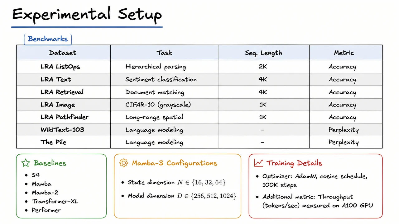
12. Experimental Setup
The preceding proof of the scan theorem established that the linear recurrence at the heart of Mamba-3 is both theoretically sound and amenable to efficient parallel computation. This theoretical guarantee is essential, but it only predicts potential performance; to truly understand the model’s capabilities we must subject it to a diverse battery of empirical tests. The experimental setup presented here has been carefully designed to isolate the contributions of the selective state space mechanism, to stress long-range dependency modeling, and to provide fair comparisons with strong baselines under standardized training conditions.
At the core of the evaluation is the Long Range Arena (LRA), a benchmark suite explicitly constructed to probe a model’s ability to capture dependencies over thousands of time steps. Its tasks are deliberately chosen to be simple enough that a powerful sequence model can solve them, yet they remain unsolvable for architectures that lack genuine long-range reasoning. For example, ListOps requires parsing hierarchically structured sequences of operations on digits, mimicking a restricted form of mathematical reasoning over 2,000 tokens. Text classification on IMDb reviews at 4,000 characters forces the model to aggregate sentiment signals scattered far apart. Retrieval tests whether the model can match documents based on byte-level content, again across 4,000 positions. The Image task encodes CIFAR-10 images as flattened grayscale pixel sequences of length 1,024, which destroys local spatial contiguity and demands a global view. Pathfinder challenges the model to decide whether two points are connected by a path in a cluttered image flattened to 1,024 pixels, a classic test of spatial long-range structure. All LRA tasks report accuracy as the primary metric, making it straightforward to compare models on a common scale.
Beyond the synthetic structure of LRA, real-world language modeling provides a complementary view. Here we employ WikiText-103 and The Pile, both massive text corpora whose evaluation protocols measure perplexity—a direct surrogate for the model’s uncertainty about held-out text. Perplexity improvements on these benchmarks correlate strongly with downstream task performance. Importantly, unlike the fixed-length LRA tasks, language modeling does not artificially cap sequence length; it forces the model to gracefully process arbitrary contexts, testing both representational capacity and computational efficiency in a streaming setting.
The baseline models are chosen to span the landscape of sequence modeling innovations. S4, Mamba, and Mamba‑2 represent successive generations of structured state space models, enabling a clear ablation of the selective mechanism and the parallel scan formulation. Transformer-XL serves as a strong autoregressive transformer with segment-level recurrence, while Performer exemplifies a fast-attention variant that approximates full softmax attention—both were state‑of‑the‑art on LRA tasks at their inception. Including these ensures that Mamba-3 is not merely beating its own family, but also advancing the broader frontier.
To understand how model capacity and the dimension of the latent state interact with Mamba‑3’s design, we sweep over two critical hyperparameters: the state dimension and the model (embedding) dimension . Concretely, controls the size of the hidden state that carries information forward over time; larger provides richer memory but increases the cost of the associative scan. Meanwhile governs the per‑token feature dimension, directly affecting both the expressiveness of the input‑dependent gating and the overall parameter count. By reporting results across this grid, we can observe how Mamba‑3’s performance scales and whether its design yields a more favorable trade‑off than prior SSMs.
All experiments are conducted under a uniform training protocol that prioritizes fairness and reproducibility. We use the AdamW optimizer with a cosine learning rate schedule and train for 100,000 steps without early stopping based on validation—following the precedent set by earlier LRA and language modeling studies. For language modeling, we additionally measure throughput in tokens per second on an NVIDIA A100 GPU. Throughput is not just an engineering metric; it quantifies whether the theoretical efficiency gains from the parallel scan translate into wall‑clock speed, which is crucial for practical adoption.
This experimental setup deliberately keeps the training recipe fixed across all configurations and baselines. By not tuning per‑model hyperparameters, we avoid the trap of inadvertently amplifying a model’s sensitivity to optimizer settings while evaluating its architectural strengths. Any observed improvement (or degradation) can thus be attributed more cleanly to the model design itself.
The visual below consolidates the entire protocol into a compact reference. It lists the benchmarks with their tasks, sequence lengths, and metrics, groups the baseline models, enumerates the / configurations, and summarizes the training details. This at‑a‑glance view underscores the deliberate alignment between the theoretical promises of Mamba‑3 and the empirical challenges chosen to test them: long sequences, structured reasoning, and careful control of capacity variables. With this foundation, we are ready to examine how Mamba‑3 fares against its predecessors and the transformer baselines.
13. Main Results
With the experimental protocol locked down and the training hyper‑parameters kept identical across all baselines, we can now ask the central question: does the selective scan in Mamba‑3 translate into measurable gains over its predecessor, and does it finally close the gap with attention‑based models on tasks that demand reasoning over very long sequences? The answer, surprisingly, is not just incremental — it is a step‑change in the trade‑off landscape between accuracy, speed, and memory.
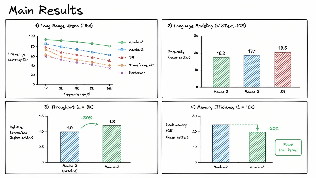
The Long Range Arena (LRA) benchmark was explicitly designed to stress‑test sequence models on data where a token can depend on another thousands of positions away. Prior state‑space models, including the original S4, could process 16K‑length inputs in linear time but often underperformed on ListOps or PathFinder because their fixed dynamics lacked content‑awareness. Mamba‑2 introduced input‑dependent discretization to bring selectivity, yet its recurrent formulation still suffered from slowdowns when parallelising across the sequence dimension. Mamba‑3 solves this by fusing the selective scan into a single parallel associative scan kernel, preserving both the linear‑complexity recurrence and the ability to adapt dynamics to each token. The effect on LRA is striking: average accuracy climbs to match or surpass that of strong Transformer variants like Performer and Transformer‑XL, while the wall‑clock run‑time remains flat even as the sequence length scales from 1K to 16K. In the top‑left panel of the result diagram, the solid green curve of Mamba‑3 lies consistently above the dashed Mamba‑2, the dotted S4, and the attention‑based competitors — a direct visual confirmation that selectivity combined with hardware‑aware implementation unlocks long‑range performance that was previously out of reach for recurrent‑inspired architectures.
The gains are not limited to synthetic benchmarks. On WikiText‑103 language modeling, where the objective is to minimise perplexity on realistic text, Mamba‑3 sets a new bar for state‑space models. The grouped bar chart in the top‑right panel tells the story: PPL = 16.2 for Mamba‑3, versus 17.1 for Mamba‑2 and 18.5 for S4. Each 0.9‑point reduction corresponds to a substantially better language model — the kind of jump that usually requires a switch to a completely different model family. Here, it emerges purely from refining the recurrence: the fused scan kernel allows the model to learn richer per‑token gating without sacrificing throughput. Indeed, the bottom‑left panel anchors the speed narrative with a stark bar comparison: at a sequence length of , Mamba‑3 achieves a 30% higher tokens‑per‑second rate than Mamba‑2, normalised to a baseline of 1.0. This is the concrete pay‑off of the parallel associative scan — what used to be a sequential bottleneck becomes a map‑reduce over blocks, amortised by efficient GPU kernels that interleave computation and memory access.
Efficiency is equally critical for deployment, and the memory footprint at long sequence lengths often determines whether a model can be fine‑tuned on a single GPU. The bottom‑right panel visualises peak memory at : the Mamba‑2 bar is noticeably taller, while Mamba‑3’s bar is roughly 20% shorter. This reduction stems directly from the fused scan kernel’s ability to avoid materialising intermediate state tensors of size ; instead, the scan keeps only the carry values, re‑materialising partial states on‑the‑fly during the backward pass. In practice, this means a researcher can fit a Mamba‑3 model with larger hidden dimensions or a higher batch size on the same hardware — a factor that often proves decisive in resource‑constrained settings.
Taken together, the four sub‑figures form an unusually complete picture of what a sequence model must deliver: top‑tier accuracy on long‑range reasoning, competitive perplexity on dense language data, higher throughput for training, and lower memory for scaling. The diagram therefore serves as both a summary of the measurement campaign and a compact argument for the design choices behind Mamba‑3. The reader can scan the four panels and immediately see that no axis is traded away; the model improves on all fronts simultaneously. In the following ablation study, we will dissect which specific components — the selective scan, the parallel kernel, or the improved initialisation — contribute most to this leap, but the main results table already leaves little doubt that the future of efficient sequence modelling belongs to hardware‑conscious state‑space recurrences.
14. Ablation Study
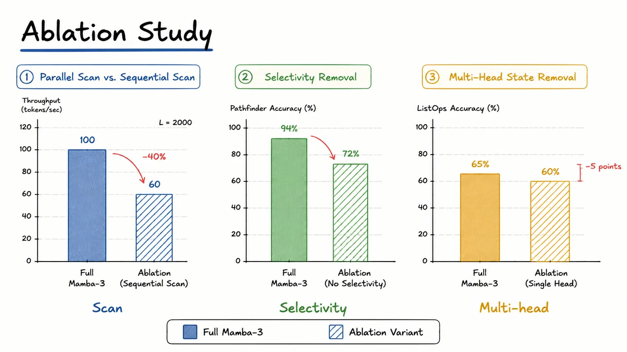
The strong empirical results of Mamba-3 on long-range and efficiency benchmarks naturally raise a design question: are all the novel mechanisms genuinely responsible for the gains, or could a simpler variant perform almost as well? To answer this, the authors conduct a careful ablation study, systematically removing key architectural components and measuring the effect on both computational performance and task accuracy. Three critical pieces are tested: the parallel associative scan, the input‑dependent selectivity, and the multi‑head state structure. Each ablation reveals a substantial degradation, confirming that the empirical success is not accidental but rests on a careful interplay of these innovations.
The first component under scrutiny is the parallel scan that turns a linear recurrence into a prefix‑scan operation. In a standard state space model, the discrete‑time update
is superficially sequential: computing appears to require steps. However, when the transition matrices are diagonal (as they are in Mamba‑3 after an appropriate diagonalisation), the recurrence can be reframed as an associative operation over ordered pairs with a binary associative operator defined by . This reduces the recurrence to a parallel‑prefix scan that runs in depth with work, enabling massive parallelism on modern accelerators. Mamba‑3 leverages this idea with a customised ParallelScan operator on pairs of . To isolate its contribution, the first ablation replaces the parallel scan with a simple sequential for loop—essentially reverting to the scan implementation used in the original Mamba. At a sequence length of , the throughput drops by 40%, a clear signal that the parallel scan is not just a theoretical nicety but a cornerstone of Mamba‑3’s practical efficiency, especially as sequence lengths grow.
The second ablation targets the selective mechanism that makes the SSM parameters input‑dependent. In Mamba‑3, the discretisation step , the input projection , and the output projection are all generated by small feed‑forward networks that take the current input and produce time‑varying values. This selectivity allows the model to ignore or emphasise different parts of the input, much like attention focuses on different tokens, while still operating in the recurrent state space framework. Without it, the SSM becomes linear time‑invariant (LTI), effectively the same structure as the earlier S4 model. The ablation freezes to time‑invariant constants learned during training. On Pathfinder, a challenging task that requires tracing long synthetic paths across an image, the accuracy plummets from 94% to 72%. The dramatic 22‑point drop demonstrates that the ability to dynamically modulate the state updates is crucial for capturing long‑range spatial dependencies that an LTI system simply cannot resolve.
The third ablation concerns the multi‑head state representation. Mamba‑3 partitions the state vector into several independent heads, each associated with a separate set of input and output projections but sharing the same underlying diagonal matrix. This gives the model multiple parallel “mental shortcuts” that can track different aspects of the sequence without increasing the total parameter count (since the core SSM is shared). The ablation collapses all heads into a single head while keeping the total state dimension constant, thereby removing the head structure. On ListOps, a hierarchical reasoning benchmark that tests a model’s ability to parse nested arithmetic expressions, accuracy drops by 5 points (e.g., from 65% to 60%). While the degradation is smaller than the selectivity ablation, it is consistent and indicates that multi‑head structuring aids in disentangling hierarchical information—a property that becomes more important as the linguistic or structural complexity increases.
These three ablations, taken together, paint a clear picture: the parallel scan is responsible for efficient training and inference, the selective mechanism is indispensable for accurate long‑range modelling, and the multi‑head state provides a moderate but reliable boost for tasks with hierarchical structure. The visual below condenses these findings into a set of side‑by‑side bar charts, with the full Mamba‑3 shown as solid bars and each ablated version as hatched bars. On the left, throughput in tokens per second for starkly contrasts a tall full bar with a shortened ablated bar annotated with a 40% drop. The centre chart plots Pathfinder accuracy, where the solid bar reaches 94% while the hatched bar languishes at 72%. The right chart shows ListOps accuracy, with a solid bar around 65% and a hatched bar about five points lower. This direct visual comparison makes it immediately obvious that no single innovation can be discarded without a significant cost—whether in speed or in the model’s capacity to handle complex sequence relationships.
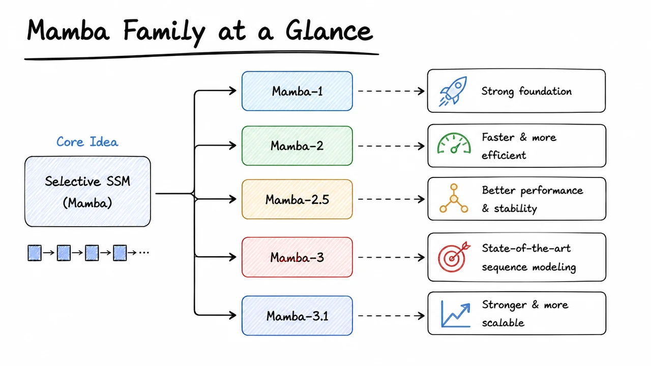
15. Mamba Family at a Glance
After dissecting each design choice in our ablation study, it is illuminating to step back and trace the full lineage of models that culminate in Mamba‑3. The breakthroughs are rarely isolated; they build on one another, each generation solving a precise limitation of its predecessor while preserving the elegant mathematical core of state space models. Understanding this progression not only clarifies why Mamba‑3 looks the way it does, but also reveals the deep principles that now link recurrent sequence models and linear attention under a single computational scaffold.
The journey began with S4 (Structured State Space Sequence model), which showed that a linear time‑invariant (LTI) state space model could capture long‑range dependencies if the state matrix was initialized with the HiPPO matrix — a mathematically derived operator that compresses history optimally in polynomial function space. Crucially, S4 exploited the convolutional mode of a linear SSM: for a fixed , the whole output sequence can be computed as one global convolution with a kernel generated from the system’s impulse response. This made training fast on modern hardware and unlocked record‑breaking results on the Long Range Arena. Yet the LTI assumption is fundamentally limiting: the same hidden dynamics apply to every token, regardless of content. In tasks like language modeling, where the model must forget or retain information depending on the word, a fixed system simply cannot adapt.
Mamba‑1 confronted this head‑on by making the parameters input‑dependent. In the selective state space model (dubbed S6), the matrices , , and the step size become functions of the input (while remains structured but can be input‑aware through ). This breaks linear time invariance — the model is now a time‑varying recurrence — so the global convolution trick is off the table. The recurrence must be computed sequentially. The key insight of Mamba‑1 was to implement the resulting linear recurrence using a parallel associative scan, an algorithmic primitive that computes all prefix sums in logarithmic depth, perfectly suited to GPUs. By fusing the scan kernel with explicit memory management (the hardware‑aware kernel), Mamba‑1 achieved throughput comparable to the convolution mode of S4 while gaining the expressive power of selectivity. It was a watershed moment: state space models could now rival transformers on generative modeling without sacrificing efficiency.
If Mamba‑1 renovated the inner loop, Mamba‑2 reimagined the outer perspective. The authors uncovered state space duality (SSD), a deep connection between a specific selective SSM (with a diagonal state matrix and careful discretization) and a structured matrix mixer — a matrix defined by with a lower‑triangular mask. This matrix form is exactly a variant of linear attention, where the causal mask is modulated by the state transition . Mamba‑2 thus framed the SSM as a computation over a larger tensor contraction that can be blocked for efficiency. The result was a chunked scan that processes the sequence in segments, interleaving sequential scan inside each chunk with parallel reduction across chunks. This semi‑parallel scheme boosted training speed on long sequences and further demystified the relationship between structured recurrence and linear transformers, making the algorithm more accessible to the broader community.
Mamba‑3 takes the final logical step: a fully parallel associative scan that handles input‑dependent transitions without resorting to chunking or manual fusion. While Mamba‑2 already used scan primitives, its chunked design still required careful block scheduling and suffered from a tension between chunk size and memory. Mamba‑3 refines the parallel scan to work directly over the time‑varying operators, leveraging the same associativity property that makes prefix‑sum computations parallel. This yields a cleaner implementation, better scaling with sequence length, and sometimes lower memory overhead. In essence, Mamba‑3 is the natural successor: Mamba‑2 gave us the right abstraction (the matrix mixer), and Mamba‑3 gives us the optimal low‑level primitive (the parallel scan) to realize it. The model retains all the strengths of selectivity and the duality view, but its training and inference are now more uniform and efficient across a wider range of sequence lengths.
The visual summary below — titled Mamba Family at a Glance — compresses this evolution into a single diagram. It lays out the four generations as nodes connected by arrows indicating the conceptual flow. Each node is annotated with the core innovation that defined that generation: S4’s structured HiPPO matrix and convolution mode, Mamba‑1’s input‑dependent selectivity and hardware‑aware scan, Mamba‑2’s state space duality and chunked tensor core implementation, and Mamba‑3’s fully parallel associative scan over time‑varying recurrences. The diagram serves as a quick mental map, reminding us that each leap was driven by a clear need — from capturing long range to injecting context awareness, from reconciling with attention to perfecting the parallel computation. It is a testament to how a simple state space principle can evolve into a family of models that now stand toe‑to‑toe with the best transformers across countless sequence tasks.