When we fine-tune language models on reasoning and problem-solving tasks where the feedback is a simple pass/fail judgment, the choice of objective fundamentally shapes which problems the model learns from. Two natural population-level objectives stand out: the expected pass rate, favored by standard reinforcement learning, and the expected log pass probability, which corresponds to maximum likelihood estimation over successful trajectories. At first glance they seem like minor variants, but their gradients reveal a dramatic difference in how they allocate learning signal across easy and hard problems.
Let denote the probability that the model, parameterized by , produces a correct answer for input . The RL objective that simply maximizes the overall proportion of solved problems is
where is the distribution over prompts. In contrast, the log-likelihood (ML) objective – often used in supervised fine-tuning where we have a set of correct demonstrations – can be written at the population level as
Both are legitimate goals, but they encode very different preferences. The RL objective rewards the model for achieving high average accuracy; it doesn’t care whether that average comes from acing easy problems while ignoring the hardest ones. The ML objective, on the other hand, penalizes the model heavily whenever a problem remains unsolved, even if it’s already extremely difficult – because is sensitive to small probabilities.
The real tension appears when we inspect the gradients. Taking the derivative under the expectation gives
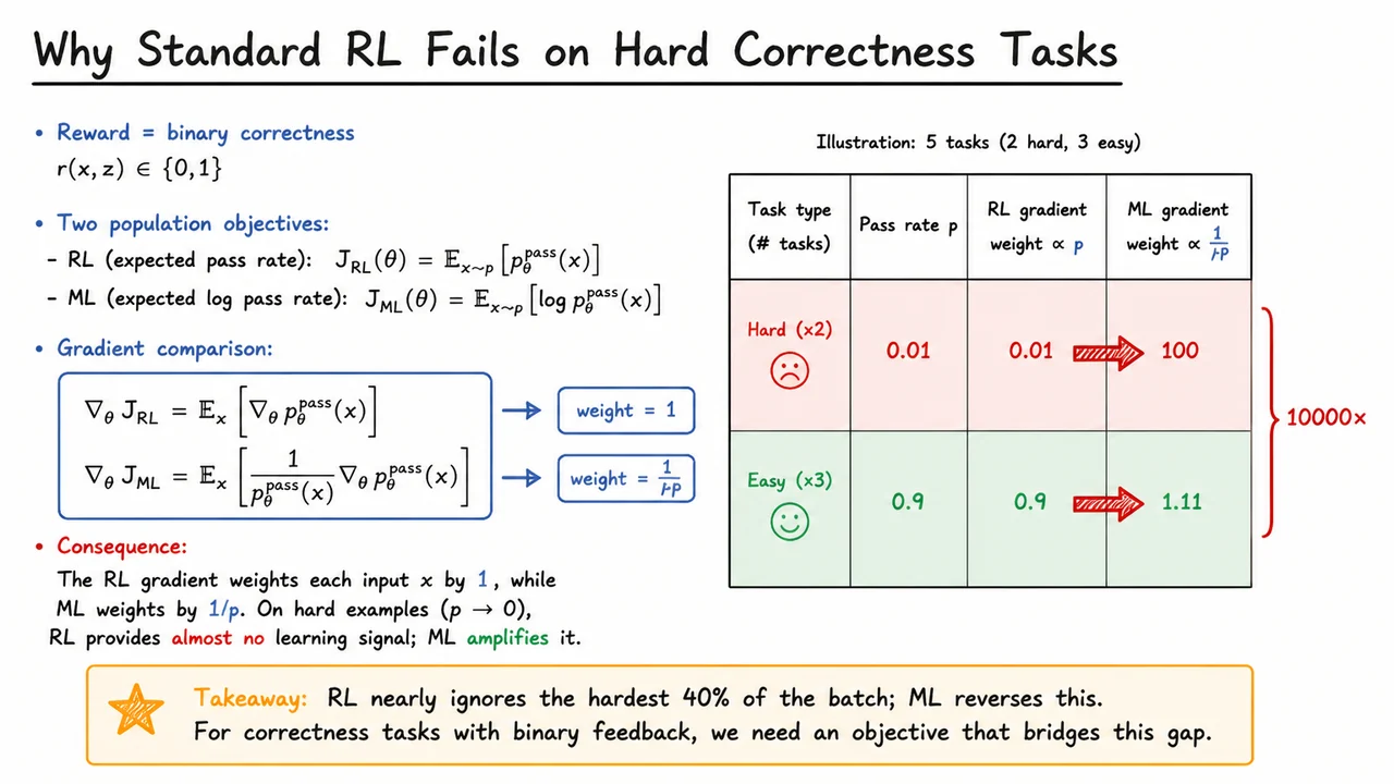
In the RL gradient, each problem’s gradient vector is weighted equally, with a coefficient of . In the ML gradient, that same vector is amplified by the inverse pass probability . Consequently, hard problems, where is tiny, receive an enormous effective weight in the ML update, while easy problems, with close to , contribute roughly the same as they do under RL. The practical outcome is a binary feedback dilemma: RL almost entirely ignores the hardest prompts, whereas ML over-amplifies them to the point of instability.
To see how severe this imbalance can be, consider a batch of five problems – two hard ones with , and three easy ones with . Under the RL gradient, the hard problems each contribute a weight of (reflecting the tiny magnitude of their relative to easier problems, or more precisely, the gradient coefficient if we rewrite ). Under the ML gradient, the hard problems are each multiplied by , while the easy ones receive a modest . In other words, the two hard problems, which together constitute 40% of the batch, are virtually invisible to the RL update, yet they dominate the ML update, receiving roughly 10,000 times the weight of the easy problems in terms of the factor applied to .
This extreme asymmetry is not just a quirk; it exposes a fundamental gap for correctness-based tasks where we have binary reward signals. Neither objective gives a principled way to control how much we care about hard examples relative to easy ones. We need a compute-indexed bridge that allows us to smoothly interpolate between these two poles – giving enough emphasis to challenging problems to learn from them, while still maintaining the stability that comes from solving a broad set of tasks. The MaxRL framework, introduced after this motivation, defines exactly such a family of objectives, controlled by a single hyperparameter that governs how many samples we invest per prompt.
The visual below – a clean diagrammatic slide titled Why Standard RL Fails on Hard Correctness Tasks – reinforces this idea at a glance. On the left, it displays the gradient equations side by side, highlighting the coefficient versus . On the right, a simple color-coded table lays out the five‑task example, with hard rows in a muted red and easy rows in green. An arrow dramatically connects the RL weight column to the ML column, underscoring the factor‑of‑ jump. The image distills the quantitative argument into a single compelling snapshot: it leaves no doubt that neither RL nor ML alone provides a satisfactory answer for binary‑correctness training, and that the missing ingredient is a tunable knob between them.
The limitations of standard RL on hard correctness tasks force us to look beneath the surface of the final answer. If the only signal a model receives is whether its decoded output matches the ground truth, then any two models that achieve identical pass rates are indistinguishable to the optimizer, regardless of how they produce their answers. To make precise statements about what an objective can and cannot recover, we need a generative model that exposes the unobserved reasoning process while still connecting to the observable binary reward. This is the latent generation model, and it is the formal backbone of the entire MaxRL analysis.
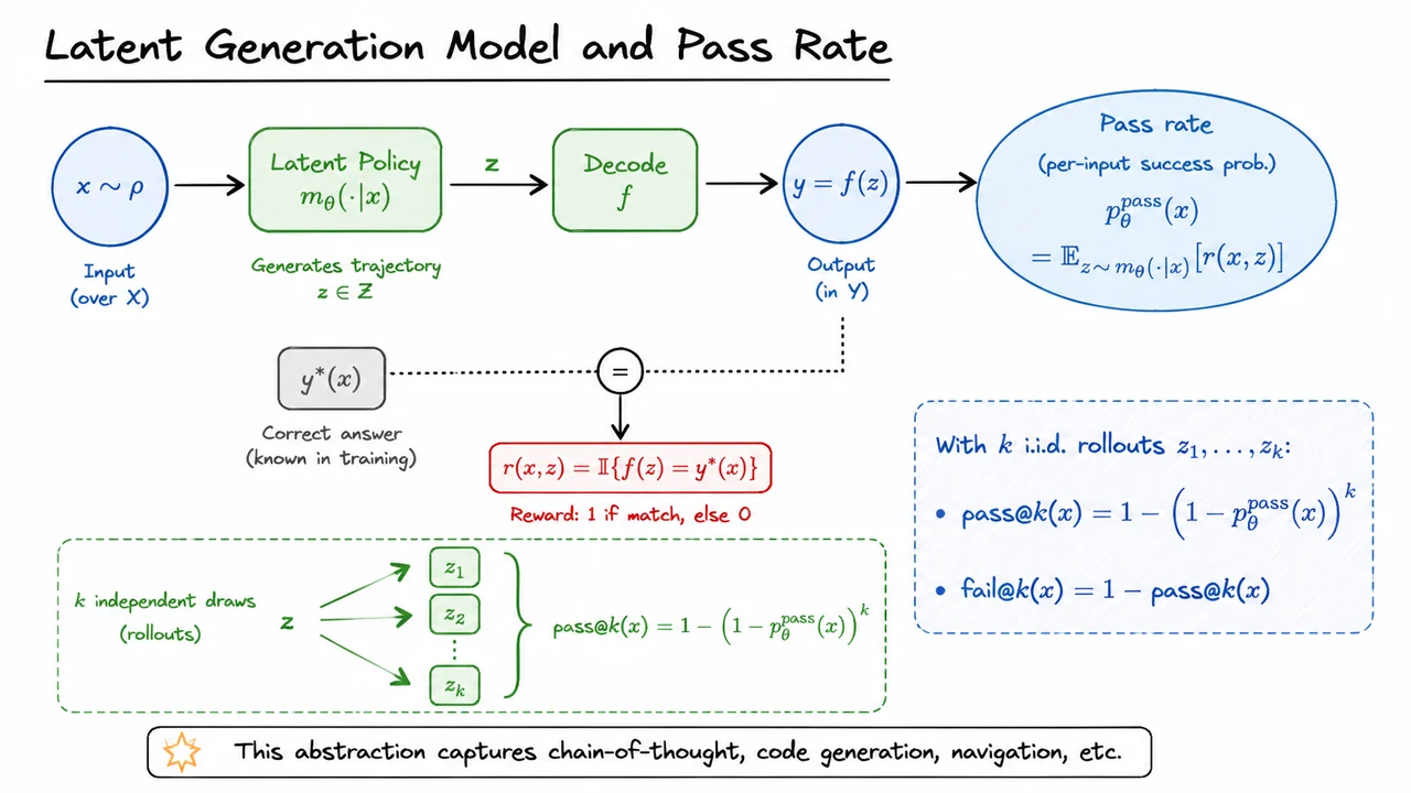
We assume an input is drawn from a distribution over a space . The model itself is a policy that, given , produces a trajectory . Crucially, is latent: it may correspond to a chain-of-thought, a sequence of tool calls, or an internal navigation plan. The model does not output directly as the user-visible answer. Instead, a deterministic decoding function maps the trajectory to a final answer . For training, we assume that for every input we know the correct answer . This abstraction is remarkably general — it accommodates mathematical reasoning, code generation, multi‑step retrieval, and any task where correctness can be judged by comparing the decoded output against a known target.
Because the decoder is deterministic, the only source of randomness in the final answer is the stochastic policy . So we can define a binary reward that indicates correctness:
This reward is all‑or‑nothing: 1 if the final answer matches, 0 otherwise. The expected reward over the model’s own latent distribution, conditioned on , is the per‑input pass rate:
In words, is the probability that a single answer obtained by sampling from the policy and then applying will be exactly correct. It is the fundamental quantity that standard RL methods optimize — but as we saw earlier, optimizing only the pass rate discards all information about the latent trajectories that produced the correct output.
That latent information, however, is exactly what we need if we hope to recover the true conditional distribution over correct trajectories, i.e., maximum likelihood. The pass rate is a coarser statistic: it collapses the rich structure of into a single number between 0 and 1. Two models with radically different reasoning patterns can have the same pass rate, yet one might produce a correct answer by genuine understanding while the other might guess wildly but sometimes land on the right token sequence. Distinguishing them requires looking at the collection of trajectories, not just the aggregate success frequency.
This is where the idea of multiple rollouts enters naturally. If we draw independent trajectories , we can compute the probability that at least one of the corresponding decoded answers is correct:
The pass@k metric quantifies how compute—in the form of additional sampling—improves the chance of seeing a correct answer. If the base pass rate is tiny (say ), then with attempts we get . The complement decays exponentially in , which will later become crucial for designing objectives that connect the number of samples to the order of a Taylor‑like expansion of the log-pass probability.
Note that pass@k is still a function of the per‑input pass rate; it adds no new information about the latent trajectories themselves. However, the joint distribution of the rollouts—and in particular the number of correct answers among them—does contain stochastic information that, with the right objective, can guide the model toward high‑likelihood reasoning paths. The stage is now set to ask: how can we design a training signal that uses this richer data, ideally recovering something akin to maximum likelihood as a limiting case?
The visual below consolidates this generative story. At a glance you see the flow from input distribution, through the stochastic policy and deterministic decoder, into the binary comparator that yields the reward. The pass rate appears as the expected reward, and the separate inset shows how independent draws give rise to the pass@k formula. The color coding — blue for input/output, green for the latent policy, red for the binary reward, gray for the known target — makes the signal‑flow interpretation immediate. This diagram is not just a static definition; it will recur as the core abstraction throughout the MaxRL development, anchoring every subsequent theorem and estimator construction in the same latent generation model.
The previous post formalized the notion of a latent generation model: a policy that stochastically produces candidate answers , and a correctness oracle that judges each one. For any fixed prompt , the pass rate
captures the probability that a single attempt from the policy succeeds. From this, we can define two natural optimization targets that extract different summaries of the pass rate distribution over prompts.
The first, maximum likelihood (ML), asks: what parameters make the observed successes most probable, in the sense of maximizing the expected log pass rate? Its objective is
The second, which we will call RL, simply maximizes the expected pass rate itself:
These two criteria coincide only when every prompt has the same pass rate – a degenerate case. In any realistic setting, they drive optimization in importantly different directions, and that divergence is the pivot of this entire lecture.
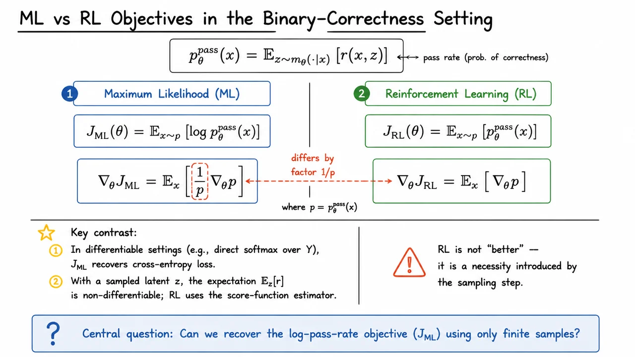
To see why, consider the gradients. Under mild interchangeability conditions we can push inside the expectation over , yielding
The RL gradient is the population version of a standard policy gradient update: it increases the pass rate wherever its derivative points, but it does so without caring about the absolute magnitude of that pass rate. A prompt with current success probability and a prompt with both receive the same gradient weight of . In contrast, the ML gradient weights each prompt’s update by , so it puts enormous emphasis on prompts where the policy is currently failing (small ), and little emphasis on those already mastered.
This contrast is not just a mathematical curiosity. In fully differentiable classification tasks – where the policy directly outputs a softmax distribution over a finite set of labels and correctness is simply the indicator of hitting the right label – the ML objective becomes the familiar cross‑entropy loss. The gradient arises naturally from the derivative of the log. However, in our setting the policy produces a latent answer and we only observe the binary correctness ; the inner expectation is not directly differentiable with respect to the policy’s parameters. To obtain a gradient estimate we must resort to score‑function (REINFORCE) estimators that use the log‑likelihood of the sampled action. That estimator inevitably introduces a term when we target the log pass rate, because the full gradient of equals and we must estimate both and its gradient from finite samples.
This is the critical point: RL is not “better” than ML; it is a practical necessity born from the sampling step. The RL objective yields the familiar policy gradient form without an explicit factor, precisely because the derivative of does not involve a weighting. That simplifies estimation enormously, but at the cost of abandoning the log‑pass‑rate criterion, which in many correctness tasks would be the principled target (it maximizes the likelihood of observing a correct answer under the latent model).
So we are left with a sharp question: Can we recover the log‑pass‑rate objective using only finite samples, without requiring knowledge of the true pass rates? The rest of this lecture frames a family of estimators that interpolate between the RL gradient and the ML gradient, indexed by the number of samples we are willing to draw per prompt. The conceptual bridge is a Maclaurin expansion of the log, which we’ll begin to unfold in the next section.
The visual below distills this tension into its bare essentials. On the left, the ML side displays the log pass rate objective and its gradient with the telltale factor. On the right, the RL side shows the expected pass rate objective and the simpler, factor‑free gradient. The two gradients are aligned to emphasize the single difference: the weighting inside the expectation. Beneath them, the key contrast is spelled out in plain terms – the differentiable case versus the sampled latent case – and the central question is boxed in blue as a prompt for the analytical bridge we are about to build.
Having seen that standard RL on binary correctness reduces to optimizing the pass probability , we might assume that scaling up RL by increasing sample budgets and reward granularity would naturally approach maximum likelihood. However, the true ML objective does not simply weight the reward by the empirical pass rate; it optimizes the log pass probability . This objective has a hidden depth: it encodes far more than the first-moment probability of a single correct answer. It distills information from the entire distribution of failures across multiple independent attempts, a structure that a pass-rate-only signal entirely misses.
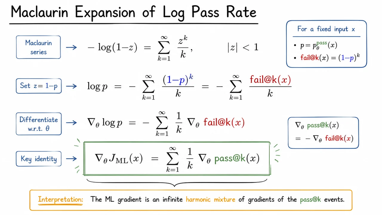
To uncover that structure, we expand through the lens of the Maclaurin series for . This classic expansion holds for and writes the logarithm as an infinite sum of powers:
Now, set , which satisfies for any . Instantly we obtain
The term is precisely the probability that all independent samples from the policy are incorrect – that is, the fail@k event, . Substituting this notation yields a crisp identity:
This series is not merely a formal manipulation; it decomposes the log-likelihood into an infinite harmonic mixture of higher-order failure probabilities. The weighting factors decay gently, meaning that fail@10 carries one-tenth the influence of fail@1, but its contribution is far from negligible.
The real power of this expansion appears when we differentiate with respect to the model parameters . Differentiating term by term – assuming standard smoothness conditions that allow the gradient to pass through the sum – we get
Each is the policy gradient of the joint failure event over samples. But since the pass event is complementary, and the gradient of the constant vanishes, we can flip the sign:
This boxed equation is the central revelation of the MaxRL framework. The maximum-likelihood gradient is an infinite harmonic mixture of the policy gradients for pass@k events. In other words, maximising automatically encourages not only that the model passes on its first try (pass@1) but also that it passes with high probability when given independent attempts, each weighted by a diminishing factor . It rewards a model that becomes robustly reliable under repeated sampling, not just a model that occasionally gets the right answer.
Why does this matter? Standard RL with a binary correctness reward produces a gradient proportional to , capturing only the first term of this infinite series. It ignores all , discarding information about whether the model overcomes its failures when given multiple tries. The ML gradient, by contrast, explicitly accounts for the full spectrum of sample budgets, revealing that the true likelihood objective inherently relies on multiple samples. This is not an ad‑hoc trick; it is a direct consequence of the logarithmic transformation.
The visual below distils this entire derivation into a clean, colour‑coded equation chain. Starting from the known Maclaurin series for , it substitutes , rewrites the powers in terms of , differentiates, and then uses the complement relation to arrive at the harmonic sum over gradients. The final identity is placed in a prominent box, with annotations that highlight the interpretation: the harmonic mixture of pass@k gradients. The use of blue for , red for fail@k terms, and green for pass@k terms makes the sign flip and the transformation visually immediate, reinforcing the conceptual shift from failure‑centered to success‑centered weighting.
With the Maclaurin expansion of established—an exact, albeit infinite, series representation of the log‑pass probability—we can now build a bridge between standard correctness‑based RL and maximum likelihood estimation. Truncating that series at a finite order produces a family of objectives that are directly controllable by a single integer parameter: the truncation length . This parameter becomes a compute index, dictating how close the objective moves toward the full log‑likelihood and, correspondingly, how many rollouts are required to obtain reliable gradient estimates.
Recall from the previous expansion that for a fixed input and model parameters , letting be the probability of generating a correct answer in one attempt, we have
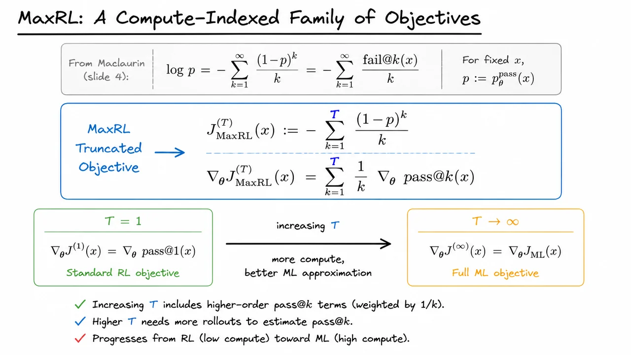
The terms decay exponentially as grows; the infinite sum is convergent, but in practice we cannot compute infinitely many terms. The truncation idea is simple yet powerful: keep only the first terms of the series and discard the remainder. For any truncation level , the MaxRL truncated objective is defined as
This is not a lower bound in the strict sense—the neglected tail is always positive, so underestimates . However, the bias shrinks rapidly with and, crucially, the gradient of has a remarkably clean form.
Differentiating with respect to (and recalling that depends on ) yields
because and , so the factor leaves . Summing the geometric series gives a compact gradient expression
From this, the weight factor directly reveals the trade‑off: it is a multiplicative damping that approaches from below as increases. When , , and the gradient reduces to , which is exactly —the standard RL objective that optimizes pass rate. As , (for ), the damping factor tends to , and the gradient converges to , the full maximum‑likelihood gradient. Thus the MaxRL family interpolates smoothly between RL () and full ML (), with every intermediate defining a partially damped gradient that approximates the ultimate log‑likelihood target.
This view re‑frames the problem as a compute‑accuracy trade‑off. Estimating for requires at least independent rollout samples to reliably assess whether any of the attempts is correct. So larger demands more samples, but it also supplies a gradient that is closer to the true ML direction. In this sense, acts as a compute knob: for a fixed compute budget one can choose the largest affordable truncation level, thereby maximising the approximation quality while respecting practical constraints.
The visual below captures this idea at a glance. It opens with a faint reference to the Maclaurin series, reminding the reader of the expansion’s structure. At the centre, a prominently boxed definition displays the truncated objective and its gradient as a sum of weighted gradients, with highlighted as the controlling index. To the sides, two parallel mini‑boxes anchor the endpoints: (standard RL, gradient driven only by ) and (full ML, exact log‑likelihood gradient). A horizontal arrow connects these extremes, labeled with the progression “increasing → more compute, better ML approximation”. Concise takeaways at the bottom reinforce the central trade‑off: larger brings the objective closer to ML but demands proportionally more rollouts. The composition makes the family’s conceptual structure immediately legible—a graded spectrum from RL to ML, with compute as the currency that determines how far along that spectrum we can afford to go.
The family of objectives we just explored—MaxRL with different truncation orders —provides a practical ladder from modest compute to ideal behaviour. But to understand precisely what those objectives are trying to approximate, and why a conditional expectation is the right building block, we need to examine the exact gradient of the maximum likelihood objective without any approximation. That gradient turns out to have a strikingly clean conditional form, something that is not immediately obvious from the definition .
Recall the starting point for any input . The ML gradient is simply the derivative of the log pass probability, This expression already hints at the need to know the pass rate itself—a quantity we cannot cheaply evaluate—but we can rewrite it into a form that eliminates the explicit division and reveals a much more intuitive structure.
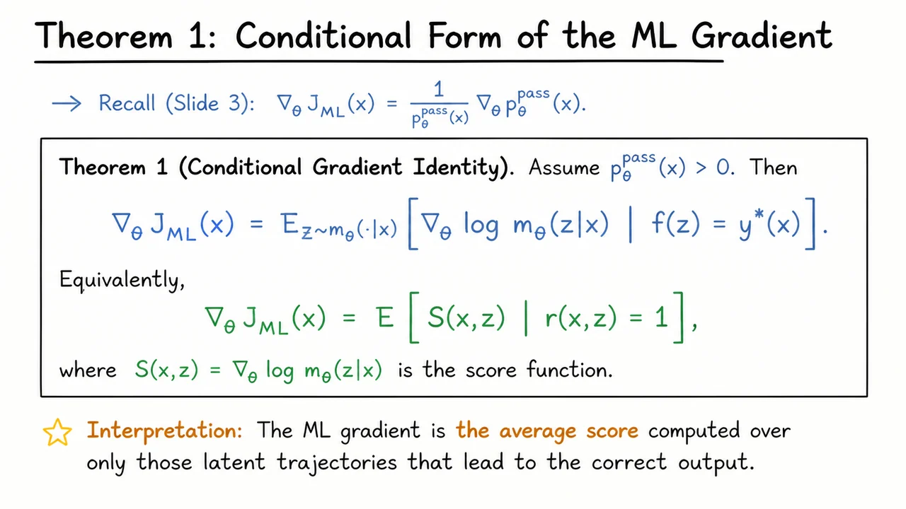
Theorem 1 (Conditional Gradient Identity). Assume . Then Equivalently, where is the score function (the gradient of the log-likelihood of a single latent trajectory).
Why is this identity both surprising and useful? In standard score-function gradient estimators (REINFORCE), we would need to multiply the score by a total reward and then divide by the marginal probability of observing that reward—so the denominator still lurks in any Monte Carlo estimate. Here, however, the gradient of the log pass probability collapses to a simple conditional expectation: the average score computed only over those latent trajectories that actually produce the correct answer. The denominator disappears because the act of conditioning on success automatically re‑weights the distribution.
The derivation is short but instructive. Expand inside the fraction: This is just the unnormalised expectation of the score function over successful trajectories. Now substitute back: The final equality uses the definition of conditional expectation: . That tiny move is what evaporates the painfully inestimable pass rate.
The assumption is not a mere technicality. It ensures the condition makes sense—there must be at least some chance of generating a correct output under the current model. In practice, for tasks with massive latent spaces, this can be satisfied early enough if we use a reasonable pre‑trained model, or we can artificially maintain a small probability mass on correctness via entropy regularisation.
Now we have a gradient that can be described purely in terms of what happens on successful rollouts. This perspective immediately illuminates a failure mode of naive RL on correctness tasks. Standard policy gradient methods (and even GRPO) optimise a surrogate that may use all sampled trajectories, perhaps up‑weighting correct ones and down‑weighting incorrect ones, but they do not exactly mimic this conditional average unless the weighting scheme matches the model’s own normalised distribution over successes. The ML gradient, in contrast, is surgically precise: take the model, sample latent trajectories, and keep only those that solve the problem. Then compute the average of their score functions. No reward‑shaping, no value baseline, no denominator—just a conditional mean.
This interpretation also explains why maximum likelihood objectives often yield models that are far more robust on reasoning benchmarks than pure RL‑tuned models. By forcing the entire gradient signal to come from correct-alone trajectories, the model learns to increase the likelihood of paths that demonstrably lead to the right answer, without being distracted by any signal from incorrect attempts. It’s a cleaner, sharper optimisation signal.
The two equivalent forms in the theorem—conditioning on and conditioning on —are simply two notations for the same event. The second form, using the binary reward , will be especially convenient when we later build finite‑sample estimators and connect to the MaxRL truncation family.
The visual below captures the essence of Theorem 1 in a compact, lecture‑ready diagram. The slide first reminds us of the starting point: the gradient of the log pass probability as a ratio. The central framed box then states the conditional identity itself, with the two equivalent expectation forms placed one above the other for immediate comparison. The use of the score notation is made explicit, and a brief interpretation line—the ML gradient is the average score over correct outputs only—sits beneath the theorem box, reinforcing the main takeaway. The hand‑drawn, academic aesthetic keeps the focus on the algebraic insight, while the clean separation of equation blocks highlights the two parallel ways of writing the same gradient. It serves as the perfect summary before we delve into the proof that formalises the connection between the conditional form and the MaxRL estimators.
Building a maximum‑likelihood objective on top of correctness feedback forces us to graduate from a naive REINFORCE gradient of pass rate to the gradient of the log‑pass probability. In the previous section we saw the population‑level identity for the pass rate:
which is a standard REINFORCE expression that weights the score by the binary correctness reward. This quantity alone tells us how to increase the probability of passing, but not how to maximise the log‑likelihood of the correct answer under the model. The jump from one to the other is the content of Theorem 1, and its proof is remarkably compact once the right algebraic relations are written down.
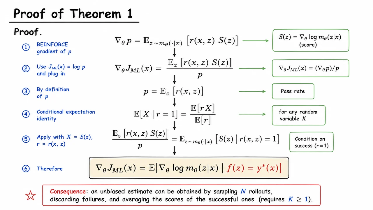
Our target is , where is the marginal pass probability. Differentiating directly gives Substituting the REINFORCE form of yields At this point everything looks like a simple ratio of expectations. The denominator is just the mean reward. So the gradient equals .
Now recall a basic probabilistic identity: for any random vector and a binary event with , the conditional expectation of given the event is This identity is nothing more than the definition of conditional expectation restricted to an event, written in terms of unconditional expectations. Its value here is that it translates a ratio of expectations back into an expected value under the success‑conditioned distribution—the distribution of model outputs that happen to solve the task.
Applying this identity with and gives That is the entire proof: a pure algebraic rearrangement that replaces the ratio of two population averages with a single conditional expectation. The right‑hand side is precisely the expected score, but only over those rollouts that actually produce the ground‑truth answer. In symbols,
Why does this matter? The gradient that maximises log‑likelihood turns out to be exactly what you would compute if you could sample only from the model’s success distribution. In other words, the ML gradient is the average score of the model on its correct answers. This immediately suggests a practical finite‑sample estimator: draw unconditional rollouts, keep the ones that pass, and average their scores. That estimator is unbiased for the gradient of a closely related objective, as we will formalise in the next section. For now, the crucial point is that the ML gradient can be expressed without ever inverting the conditional distribution or needing a separate “teacher”—the structure is fully contained inside the model’s own pass/fail behaviour.
The visual that supports this proof serves as a minimalistic derivation map. It presents the REINFORCE expression for , the division by , the rearrangement into the ratio , and the application of the conditional expectation identity—each step appearing as a single aligned equation. The final line is the boxed theorem statement, set apart with a subtle coloured background. This depiction is not meant to replace the logic, but to consolidate it into a glance‑able chain of reasoning, making the essential move—from a ratio of expectations to a conditional mean—immediately visible. The viewer can see at a glance why “discard failures and average the scores” is the population‑level truth behind maximum‑likelihood training with binary rewards.
Having established that the gradient of the log pass probability can be expressed as a conditional expectation over successful trajectories, we now turn to its finite-sample approximation. The population-level form from Theorem 1,
naturally suggests an intuitive Monte Carlo estimator: draw latent trajectories , compute the binary rewards , count the successes , and then average the score gradients of the successful trajectories—each weighted equally. However, when no successes occur (), the conditional expectation is undefined and no learning signal can be extracted from a sample that contains only failures; in that case the estimator is simply set to zero.
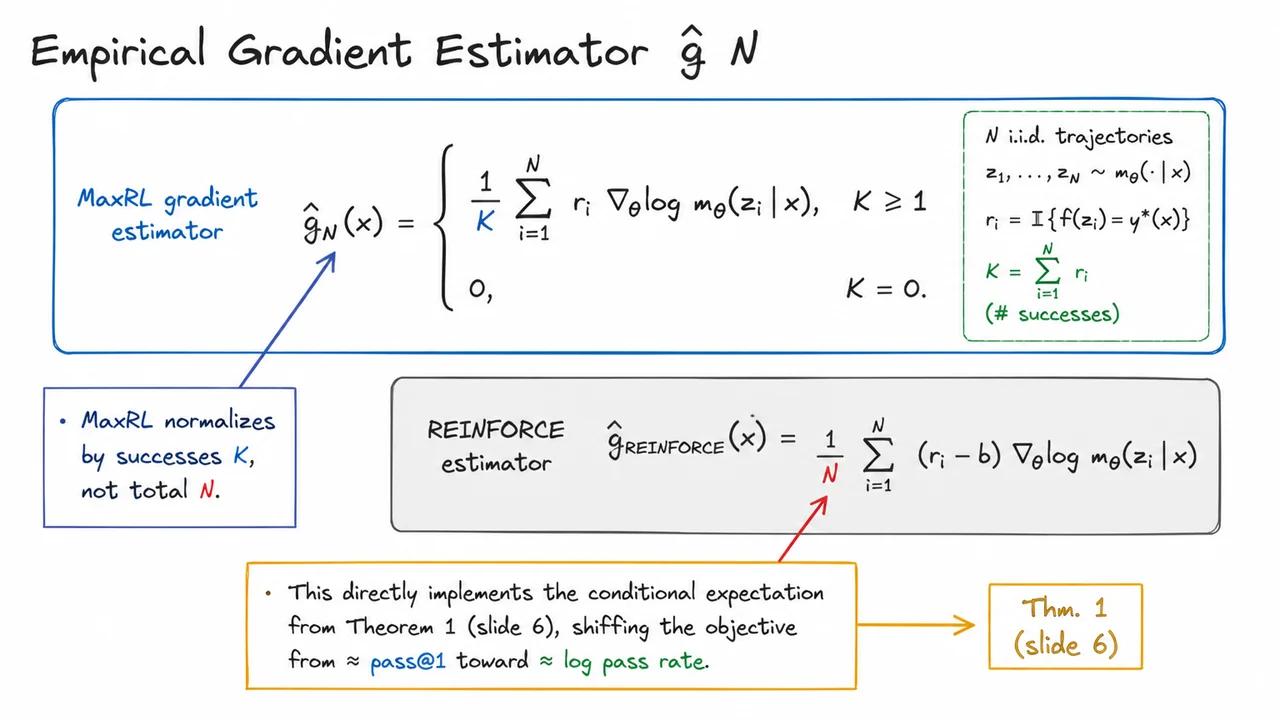
This yields the MaxRL gradient estimator:
The piecewise definition echoes the truncation-based logic that underpins the whole MaxRL framework: when the sample reveals no successes, we cannot improve the log pass probability from that mini-batch, so the update is null. When at least one success is present, the estimator uses only the successful draws, normalising by the observed number of successes rather than by the total sample size .
It is instructive to contrast this with the classic REINFORCE estimator commonly used in reinforcement learning for correctness tasks:
where is a baseline (often a learned value function or a moving average of rewards). REINFORCE estimates the gradient of the expected reward—in this binary case, the pass probability . Every trajectory, successful or not, contributes to the estimate. The baseline reduces variance but does not change the objective being optimized: REINFORCE pushes the policy toward producing any success, without distinguishing between a policy that succeeds rarely and one that succeeds reliably once we condition on some success. In other words, it optimises the pass rate (pass@1) but does not recover the maximum-likelihood principle that underpins standard supervised fine-tuning.
The MaxRL estimator replaces the uniform weighting of all trajectories with a conditional average over the successful ones. This seemingly minor change has profound consequences:
A critical subtlety is the treatment of the case. Setting the gradient to zero when no successes are found may seem wasteful, but it is perfectly aligned with the truncation viewpoint: a sample of size that contains zero successes provides no information about the higher-order terms in the Maclaurin expansion of the log pass probability. The gradient is zero because the conditional expectation is undefined; any ad‑hoc non‑zero value would bias the objective away from . This design choice is not a limitation but a deliberate bridge between sample size and truncation order that will be formalised in Theorem 2.
The visual below makes this contrast immediate. At the top, the main MaxRL estimator is displayed prominently, with its piecewise definition centred in a clean box. The handling of the two cases— and —is spelled out, emphasising the normalisation by . Immediately underneath, in a slightly smaller, shaded box, the REINFORCE estimator is shown for side‑by‑side comparison. An arrow annotation calls out the denominator: in MaxRL versus in REINFORCE, highlighting the fundamental difference in weighting. Another arrow points to a small tag referencing Theorem 1 from the preceding slide, reminding the viewer that this estimator is not an arbitrary choice but the natural sample analogue of the conditional expectation that lies at the heart of the MaxRL derivation. The muted shading of the REINFORCE box further reinforces that MaxRL is the estimator of primary interest, with REINFORCE serving as a familiar foil.
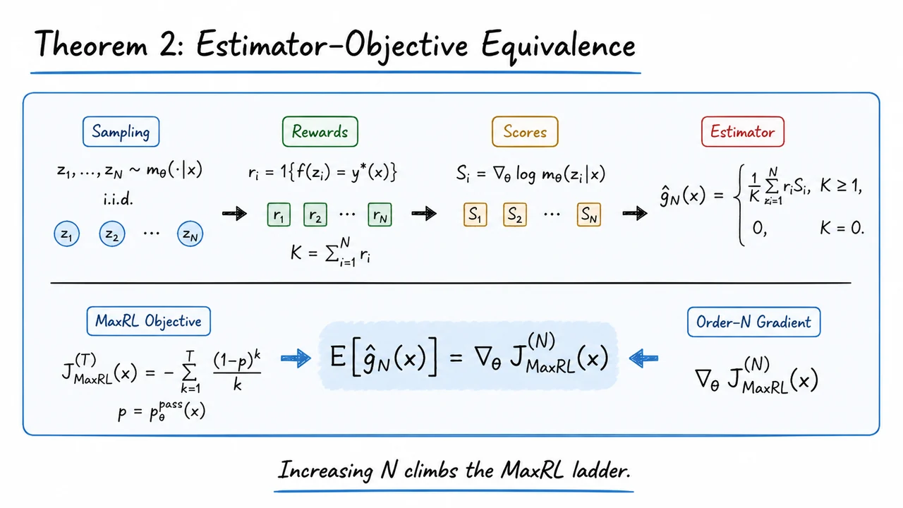
The definition of in the previous section may look like a pragmatic hack: average the score vectors of correct rollouts, ignore all failures, and return zero when nothing succeeds. Yet there is a strikingly clean reason that this particular ad‑hoc construction works. Theorem 2 uncovers the exact objective whose gradient is estimated without bias by . It reveals that the estimator is not just a clever trick but a direct conduit to the truncated Maclaurin series of the log pass probability – the very series we derived earlier when expanding .
Theorem 2 (Estimator–Objective Equivalence).
For any integer and any prompt , draw i.i.d. completions . Let indicate correctness, be the score, and count successes. With
and the MaxRL objective of order
the expectation over the rollouts satisfies
To appreciate the claim, recall that the Maclaurin expansion of in powers of is
Thus is exactly the -th order truncation of the true log-likelihood of correctness. When we later aggregate over a training set of prompts, maximising the full log-likelihood is the standard MLE target. The theorem therefore asserts that each invocation of is an unbiased Monte Carlo estimate of the gradient of a truncated version of that MLE objective – and the truncation order automatically equals the number of rollouts we have just drawn.
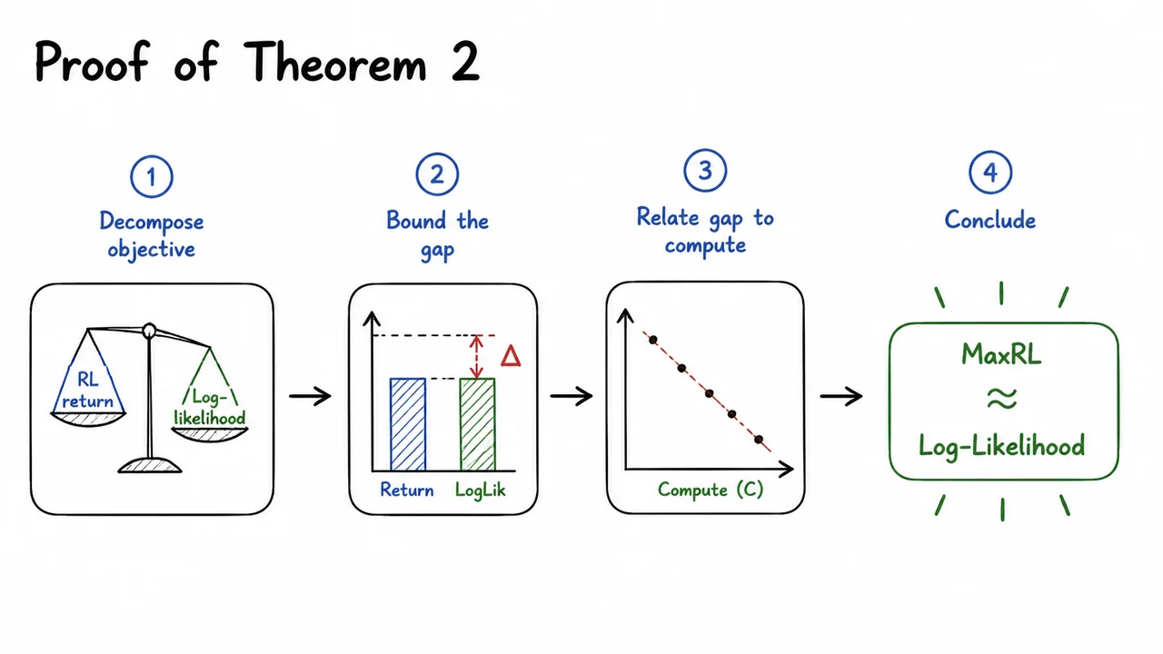
Why should this hold? The proof (explored in the next section) hinges on a delicate cancellation. The naive approach would be to compute by differentiating term by term, which produces a sum involving powers of and the gradient of . Instead, the estimator averages scores only over successes and divides by the empirical success count . When you condition on the number of successes , the conditional expectation of over the successful trajectories, together with the binomial probabilities for , miraculously collapses into exactly the derivative of the finite sum. The case contributes zero, which aligns with the fact that the derivative of the series vanishes when (the constant term is , a constant independent of ).
The practical consequence is profound. We never need to manually decide what truncation order to use or to store explicit representations of the series. Simply drawing rollouts and calculating the empirical correct‑average score produces a gradient that, in expectation, corresponds to a specific point on the ladder of Maclaurin approximations. For , , which is exactly the standard REINFORCE gradient for the pass‑rate objective (RL). As grows, the expected gradient moves continuously toward , the gradient of the full maximum‑likelihood objective. The estimator therefore builds a compute‑indexed bridge: the more rollouts you can afford, the closer you drive the model to maximum likelihood on the correctness task – without any change in the algorithmic mechanism.
In teaching, this equivalence is often presented as a compact, boxed statement that isolates the theorem from the surrounding algebra. The visual below captures that style: a centered theorem box containing the crucial equation , together with a minimal italic remark beneath – “Increasing climbs the MaxRL ladder.” This one‑liner distills the core insight that more compute automatically lifts the objective towards ML, making the ladder metaphor a handy mnemonic for the entire MaxRL framework.
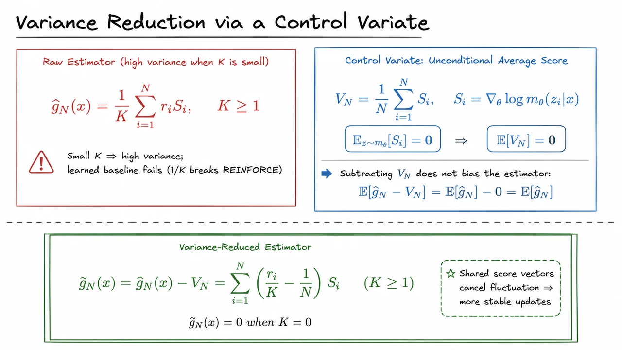
The previous section proved that the population gradient for MaxRL is exactly the expectation of a truncated score-weighted sum, which yields a natural finite‑sample estimator . The proof established that the estimator is unbiased, but it did not address its variance—which turns out to be the central practical obstacle when we actually draw on‑policy trajectories. We must now face the fact that for challenging correctness tasks, , the number of successful completions in a batch, can be very small. The raw estimator
and zero otherwise, inherits an acute instability: the division by the random count amplifies fluctuations, especially when takes values like 1,2,3. In those regimes, a single extra success or failure drastically changes the weight , causing large jumps in the gradient estimate. Variance reduction therefore becomes essential for any on‑policy implementation that hopes to converge reliably.
A natural first thought is to borrow the classic REINFORCE baseline trick. In standard policy gradients, we can subtract a state‑dependent baseline from the return without biasing the gradient, because the score has zero expectation: . Here, however, the normalisation by breaks that property. The weight is a random variable that depends on all drawn solutions, making it correlated with the scores in a nontrivial way; a simple baseline no longer yields a zero‑mean correction. We need a control variate that remains incontrovertibly zero‑mean regardless of the mixture of successes and failures.
The solution is elegant and easy to compute: use the unconditional average score over all samples, with no reference to correctness. Define
Because the score function always has zero expectation under the sampling distribution, , we immediately obtain , for any and any policy. This zero‑mean property holds exactly, no matter the batch composition; it does not rely on independence from the rewards. Subtracting from the raw estimator therefore cannot introduce bias:
Thus, remains an unbiased estimator of the gradient of .
Now we can write the combined estimator in a revealing form. When ,
and when . The per‑sample weight shifts from to . For a correct sample () this weight becomes ; for an incorrect sample () it becomes . The weights now sum to zero across all draws, because . This zero‑sum property effectively removes the baseline drift that plagues the raw estimator. Intuitively, the control variate captures the aggregate random fluctuation of the score vectors, and because the same vectors appear in , subtracting cancels a large portion of the stochastic noise—especially when is small and can be large in magnitude.
The diagram that accompanies this section distills the construction into a compact visual. The left column presents the raw estimator in red, marked with its high‑variance affliction for small . The right column displays the control variate in blue, with an arrow pointing to the key property . A horizontal dashed line separates these building blocks from the final result below: a double‑bordered box in dark green containing the variance‑reduced estimator . A small italic note reminds us that the estimator gracefully falls back to zero when . The colour coding and spatial layout reinforce the logical flow: we start from a noisy but unbiased estimate, subtract a zero‑mean companion that shares its stochastic source, and obtain a stabilised estimator that remains unbiased and is far more practical for iterative on‑policy training. This control variate trick turns Theorem 2’s unbiased estimator into a tool we can actually deploy, setting the stage for the complete on‑policy algorithm that follows.
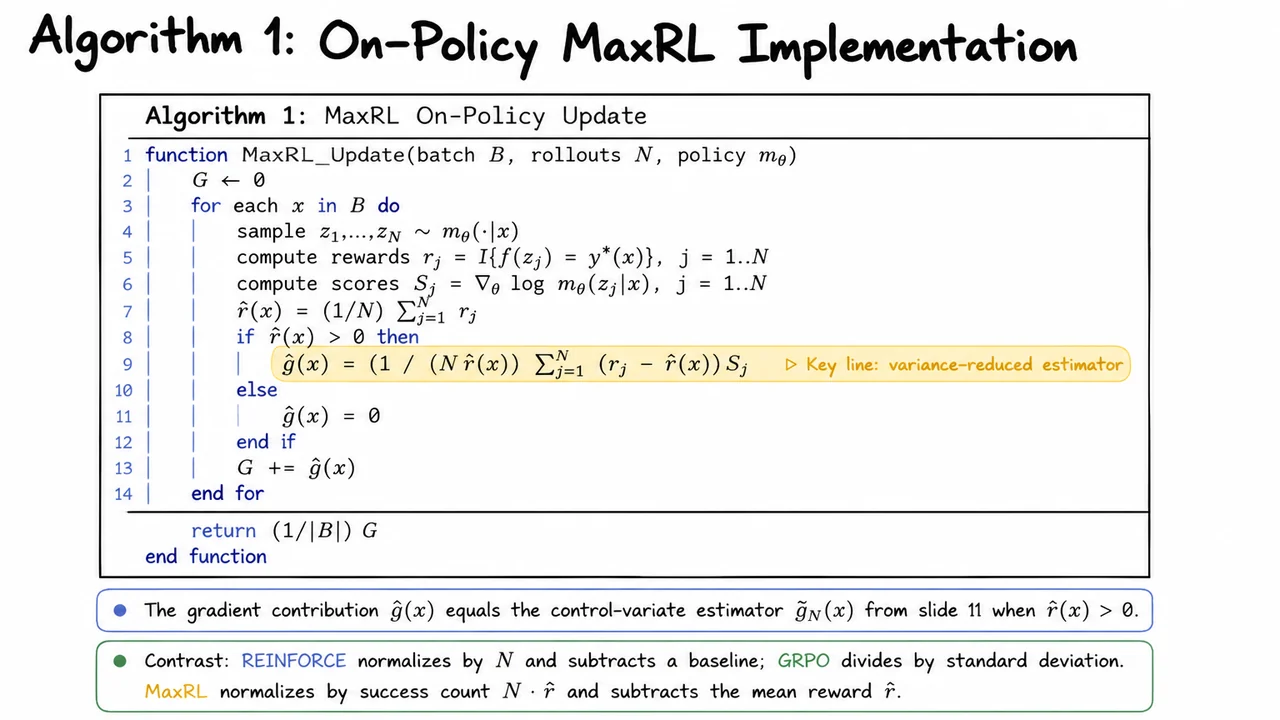
With the control‑variate estimator fully derived, the next step is to embed it inside a practical training loop. The result is Algorithm 1, an on‑policy update that replaces the usual REINFORCE gradient with a variance‑reduced contribution for each input . The algorithm is simple to implement, yet its structure directly realises the truncated log‑likelihood objective we recovered from the Maclaurin expansion.
For a batch of inputs , the algorithm samples responses from the current policy for each , evaluates the binary correctness reward , and records the score vectors . The crucial step is forming the empirical success rate and then computing the gradient contribution whenever ; otherwise . Comparing this with the standard REINFORCE estimator reveals two fundamental differences: the denominator is the total number of successes rather than , and the baseline is the per‑input empirical mean instead of an exogenous baseline. Both modifications arise directly from the derivation; they are not heuristic tweaks.
The normalisation by is what ties the algorithm to maximum likelihood. Recall from the expansion of that the -th term involves the conditional expectation over the successful trajectories only. In the estimator , the sum is equivalent to . When we divide by , we are effectively forming the estimator which is a consistent sample approximation of . The first term is the gradient of the log‑likelihood restricted to correct completions, while the second term (the average over all samples) acts as a control variate whose expected value is zero under the policy. Thus the estimator is targeting the truncated log‑likelihood objective—it pushes the policy toward distributing mass only among correct responses, exactly as demanded by the full MLE solution when all responses are correct.
The condition is a practical safeguard. If the policy never produces a correct answer for a given input within the samples, then there is no information about which directions would improve correctness, and the gradient contribution is set to zero. This prevents the update from being corrupted by division by zero and, more importantly, avoids misleading the policy when it is completely unsuccessful. It also reflects the truncation order: if no successes are observed, the corresponding term in the Maclaurin expansion would vanish, so the estimator stays coherent.
After accumulating across the batch, the final update direction is simply . This is a standard stochastic gradient step that averages gradient contributions over the batch. Note that the sampling of completions per input is done on‑policy, so the rollouts must be re‑drawn after each parameter update to maintain consistency with the current policy—exactly as in any REINFORCE‑style algorithm.
The algorithm’s design highlights the role of as a compute‑indexed knob. When , can only be 0 or 1, and the estimator collapses to when (zero otherwise). As grows, the estimator concentrates around the true truncated gradient, reducing variance and enabling finer‑grained updates that approach MLE behaviour. Later we will see that the sample count directly corresponds to the truncation order in the objective, making the compute budget an explicit parameter that interpolates between RL and pure log‑likelihood training.
It is also instructive to contrast MaxRL with GRPO, which normalises the reward by the standard deviation of rewards within a group of rollouts. GRPO subtracts the group mean and divides by the group standard deviation to measure advantage, an approach that works well for scalar reward shaping but does not target a log‑likelihood objective. MaxRL, by using the per‑input success fraction as both baseline and normaliser, recovers the exact gradient of a truncated log‑likelihood when rewards are binary and the success probability is non‑negligible.
The accompanying slide provides a compact, at‑a‑glance summary of these ideas. A central pseudocode block faithfully renders Algorithm 1, with the line computing highlighted—this is the key line that embodies the variance‑reduced estimator we have just deconstructed. Beneath the block, two concise bullet points contrast MaxRL with REINFORCE and GRPO: one notes that REINFORCE normalises by and subtracts a baseline, while MaxRL normalises by success count and subtracts the mean reward ; the other points out that GRPO divides by standard deviation, whereas MaxRL’s normaliser is tied directly to the sample success rate. These contrasts crystallise the implementation differences that make MaxRL distinct, turning the slide into a quick reference for anyone implementing the method.
Having implemented MaxRL as an on‑policy procedure in Algorithm 1, we now have a concrete algorithm that uses multiple independent attempts to construct an unbiased gradient. But stepping back, it becomes clear that MaxRL is not an isolated trick—it sits inside a broader family of methods that share a common mathematical skeleton. All of them can be understood as different ways of choosing how much to amplify the gradient signal from a prompt based on the model’s current pass probability . This suggests a simple, unifying language: a weight function that scales the per‑example gradient . Once we adopt this view, the design space of policy‑gradient algorithms for correctness tasks collapses to selecting the weight function , and we can compare methods side‑by‑side by looking at their weight curves.
The shared template is deceptively compact. Let denote the distribution over prompts (or more generally the state visitation distribution under the current policy). Then the gradient of any objective that factors through the pass probability can be written as
The weight function encodes the objective’s sensitivity to examples of different difficulty. An example where the model nearly always succeeds () and an example where it nearly always fails () can receive drastically different weights depending on the method. The template itself is a direct consequence of the policy gradient theorem when the per‑step reward is replaced by a binary correctness signal, but the real value is that it decouples the scale of the update from the raw probability, allowing us to design algorithms by reasoning about in isolation.
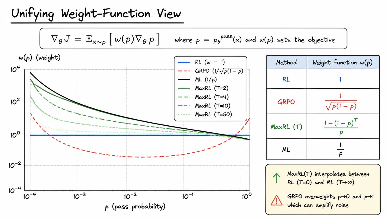
Standard reinforcement learning—the most common baseline—treats every completed trajectory equally: a correct answer yields a reward of 1, an incorrect one 0. Under this reward scheme the expected return is the pass probability, and its gradient reduces to , i.e., . This constant weight ignores how certain the model already is about a prompt. An easy prompt contributes exactly as much gradient as a borderline one, which is wasteful when many gradient samples are dominated by high‑probability noise. GRPO, the method used in DeepSeek‑R1, attempts to remedy this by normalising rewards within a group of rollouts. Its effective weight function becomes the reciprocal of the standard deviation of the binary outcome: . This function is symmetric and strongly U‑shaped—it heavily upweights prompts where or because those are the cases with the smallest variance. While this gives maximal weight to confidently correct or confidently wrong answers, it also amplifies noise, since the variance estimate itself is unstable for extreme probabilities.
At the opposite extreme sits maximum likelihood estimation over correct trajectories. Maximising log‑likelihood of correct answers—or, equivalently, minimising the cross‑entropy loss on only positive examples—gives a gradient of the form , so . This hyperbola is gentle for easy prompts ( near 1, weight near 1) but grows without bound as shrinks, desperately trying to lift the tiniest success probabilities. It is compute‑hungry because it needs reliable estimates of on very rare successes, which usually requires millions of samples. MaxRL bridges these extremes. Its weight function, derived from the truncated Maclaurin expansion of , is
For this reduces to (since ), while as it approaches for any , recovering ML. At finite , the function behaves like when is large because decays quickly, and it smoothly bends upward toward the ML hyperbola as becomes small. This interpolation is controlled solely by the truncation order , which equals the number of independent attempts used in the MaxRL estimator—a direct compute‑indexed bridge.
Viewing all four weight functions on a single log‑log plot makes the relationships immediate and intuitive. The x‑axis is the pass probability , spanning several orders of magnitude from near‑impossible prompts to near‑certain ones. The y‑axis is the weight , also on a logarithmic scale to expose power‑law behaviour. In such a visual, RL appears as a flat horizontal line at —utterly indifferent to . Maximum likelihood traces a straight line with slope (since ), a hyperbola that skyrockets for tiny . GRPO forms a symmetric bowl that rises sharply at both ends, visually distinct from everything else. The MaxRL family fans out between RL and ML: for the curve barely lifts above 1 except at the very lowest probabilities; bends significantly earlier; hugs over a wide range before saturating at for . This saturation is the key—MaxRL never overweights hopeless prompts as severely as ML does, because the truncation caps the weight at . The plot also reveals a subtle danger: GRPO’s peak at can be far larger than any MaxRL curve for confident successes, potentially causing overfitting to already‑mastered prompts instead of focusing compute on the tail. In contrast, MaxRL concentrates gradient credit on the examples that are neither impossible nor already solved, which matches the intuition of efficient learning.
The visual below distills the entire discussion into a single, glanceable comparison. The four families are colour‑coded and a legend identifies each by its functional form. The family of MaxRL() curves, plotted for , visibly threads the needle between the flat RL baseline and the steep ML target, illustrating how the hyperparameter indexes a smooth trade‑off. The log‑log axes make it obvious that the weight functions differ most dramatically in the low‑probability regime, precisely where data scarcity forces an algorithm to choose between high variance and high bias. This unified weight‑function view not only organises existing methods but also suggests new ones: any monotonically decreasing with controlled growth near zero could be a candidate for compute‑efficient reinforcement fine‑tuning, and this plot gives us the mental model to design it.
With a unified weight-function view of the optimization landscape, the theoretical promise of MaxRL becomes concrete: by indexing the gradient estimate with a truncation order , the algorithm interpolates between a raw reinforcement signal and the exact maximum-likelihood gradient. The natural next step is to validate whether that interpolation translates into genuine empirical gains—especially in regimes where existing methods are known to struggle. The empirical highlights across image classification, spatial reasoning, mathematical problem-solving, and large-scale language model fine‑tuning all point to the same conclusion: MaxRL consistently outperforms REINFORCE-style baselines and the popular GRPO family, often by dramatic margins.
Recall the core predicament that standard policy‑gradient methods face on correctness tasks. When a binary reward only flags whether a sampled answer is correct, the gradient estimator is fundamentally limited to the support of positive rollouts. In problems with a low initial pass rate, that support can be extremely sparse; the resulting signal is weak, high‑variance, and entirely blind to the structure of incorrect answers. REINFORCE and its modern derivatives (RLOO, GRPO) consequently stall in these cold‑start conditions—they simply do not see enough correct traces to climb out of the low‑performance basin. MaxRL sidesteps this trap by exploiting the Maclaurin expansion of the log‑pass‑probability: instead of ignoring negative rollouts, it weights them according to a truncated exponential series that automatically assigns meaningful learning signals to both correct and incorrect samples. The truncation order becomes a compute‑indexed dial that, when turned up, recovers the full log‑likelihood gradient with exactness.
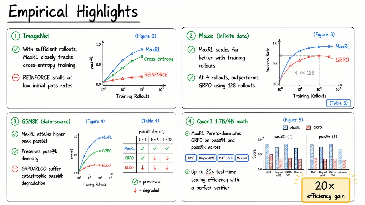
The first striking demonstration comes from an ImageNet classification proxy, where the model is trained from a low initial pass rate. Standard REINFORCE plateaus early—its reliance on sporadic positive examples prevents convergence toward the cross‑entropy teacher. MaxRL, in contrast, closely tracks the cross‑entropy baseline as the number of rollouts per sample grows (Figure 2). This is a direct consequence of Theorem 2: with rollouts, the finite‑sample MaxRL estimator exactly implements the ‑truncated Maclaurin term of the log‑pass‑probability. As increases, the objective smoothly morphs into a proper maximum‑likelihood loss, explaining why it can eventually match cross‑entropy performance. The experiment thus confirms that MaxRL’s compute‑indexed bridge is not just a formal curiosity but a practical mechanism for escaping the cold‑start trap.
Equally telling is a Maze navigation task with access to effectively infinite training data. Here the question is not data scarcity but gradient efficiency: how many environment interactions are needed to reach a strong policy? MaxRL scales far more gracefully with the number of training rollouts than GRPO does. Notably, MaxRL with only 4 rollouts per problem instance already outperforms GRPO using 128 rollouts (Figure 3, Table 3). This counter‑intuitive result makes sense through the weight‑function lens. GRPO applies a severe advantage‑clipping operation that discards fine‑grained credit assignment among rollouts, effectively compressing the information into a crude relative‑ranking signal. MaxRL’s weight function, being a smooth polynomial in the pass rate, preserves richer per‑sample feedback even with a small rollout budget, so it needs far fewer samples to build an accurate gradient. Empirically, this translates into a massive reduction in required compute.
Perhaps the most dramatic warning for practitioners comes from the GSM8K data‑scarce regime. Here, fine‑tuning a language model on only a handful of math word‑problem chains reveals a dark side of optimizing solely for pass rate. GRPO and RLOO drive the model to high pass@1, but they simultaneously suffer catastrophic pass@k degradation: the set of valid solution paths collapses, and the model loses the diversity that makes test‑time majority voting effective (Figure 4, Table 4). MaxRL achieves a higher peak pass@1 while preserving pass@k diversity—the distribution over correct reasoning chains remains rich. This is exactly what we would expect when the objective approximates maximum likelihood rather than a mode‑seeking RL signal. The truncation order acts as an implicit regularizer; even with finite , the log‑probability target encourages coverage of all correct modes, not just the easiest one. For safety‑critical or reasoning‑intensive tasks, that property is invaluable.
The modern scale test cements the case. Fine‑tuning Qwen3 1.7B and 4B models on mathematical benchmarks (AIME, BeyondAIME, MATH‑500, Minerva) with a perfect outcome verifier reveals that MaxRL Pareto‑dominates GRPO on both pass@1 and pass@k across all tasks (Figure 5). The dominance is particularly tangible in test‑time compute scaling: when allowed to sample and majority‑vote at test time, models trained with MaxRL achieve up to a 20× efficiency gain over GRPO‑trained counterparts. In other words, to reach a target accuracy, a MaxRL model needs 20 times fewer test‑time samples, directly capitalizing on its preserved distributional diversity. The visual below captures this cluster of results in a 2×2 grid of summary bullet points, with green‑coded successes where MaxRL excels and red‑coded pitfalls for competing methods. A dedicated highlight box underscores the 20× test‑time scaling advantage, reminding us that the bridge from RL to log‑likelihood is not merely an academic equivalence but a recipe for substantially better sample efficiency at both training and inference time.
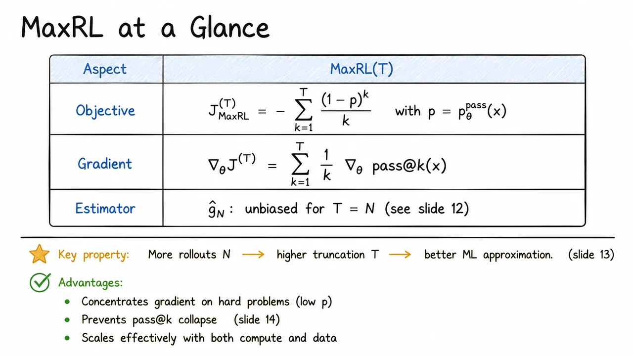
The empirical results we just examined show a striking pattern: a model fine-tuned with a simple reinforcement learning reward—answer correctness—can boost its pass rate on held-out prompts, yet it often fails to capture the full statistical richness of the data. The learned policy may ignore subtle failure modes, become overconfident, and ultimately leave a gap when we measure its log-probability rather than the binary pass rate. This raises a deeper question: can we design a family of objectives that, at low compute, behaves like an RL pass-rate maximizer but, as we increase the number of samples, converges to the maximum likelihood estimate? Maximum Likelihood Reinforcement Learning (MaxRL) does exactly that by carving a compute-indexed path from the binary reward world to the log-likelihood ideal.
The key mathematical observation is that for any prompt and any evaluation protocol that ultimately extracts a binary correctness outcome, the model’s pass probability satisfies
a Maclaurin series that converges for . Truncating this expansion after terms yields a family of surrogate objectives
where we treat as the quantity to be optimized over the policy parameters. When , , a linear function of the pass rate; maximizing it is equivalent (up to an additive constant) to maximizing the expected binary reward—standard RL on correctness. For , higher-order terms—the pass@k probabilities that at least one of sampled answers is correct—enter the objective, and they become increasingly influential when is small. In other words, the truncation order acts as a dial that controls how far we push beyond a single binary success toward the full log-probability surface.
Gradient-based optimization is made practical by the following identity (Theorem 1 of the MaxRL derivation):
Each term can be estimated without bias from a finite number of rollouts. Crucially, when we draw independent rollouts per prompt and construct the natural estimator (described earlier in the lecture), that estimator is unbiased for . Thus the rollout count directly sets the effective truncation order: with samples we are, in expectation, optimizing . This compute-indexed link is the heart of MaxRL—the level of sampling determines which member of the objective family we are actually pursuing.
Why does this matter? As we increase , the objective progressively incorporates pass@k terms for larger , each weighted by . Hard problems, where the pass probability is low, see relatively larger contributions from higher-order terms because tends to be more pronounced when the model struggles to get any sample correct. The gradient thus concentrates on the most difficult prompts, preventing the model from simply learning a uniform “easy mode” strategy. At the same time, the explicit dependence on pass@k for discourages pass@k collapse—a degenerate behavior observed in vanilla RL where the policy becomes deterministic and all attempts produce the same (possibly wrong) answer, making pass@k estimates unreliable and learning stale. With MaxRL, even if pass@1 is high, the model retains incentive to produce diverse correct solutions, because any failure to achieve at least one correct answer among trials is penalized by the terms.
Taken together, the MaxRL framework cleanly unifies pure RL, maximum likelihood, and a spectrum of intermediate objectives under a single weight-function perspective (when compared to GRPO and similar algorithms, MaxRL can be seen as adjusting the sampling weight according to truncated at order ). The visual summary below condenses this unified view into a compact table, listing the core objective, its stochastic gradient, and the unbiased estimator that realizes the truncation via rollouts. Below the table, highlighted bullet points reinforce the compute-indexed property—more samples imply a higher truncation and a better ML approximation—and the practical advantages: concentrating gradient on hard examples, preventing pass@k collapse, and scaling effectively with both compute and data. This at-a-glance reference grounds the more detailed theorems we have explored and serves as a quick mental model for why MaxRL behaves as a smooth bridge from simple reward maximization to full log-probability learning.