Mechanistic Interpretability: Reverse-Engineering the Algorithms Inside Neural Networks

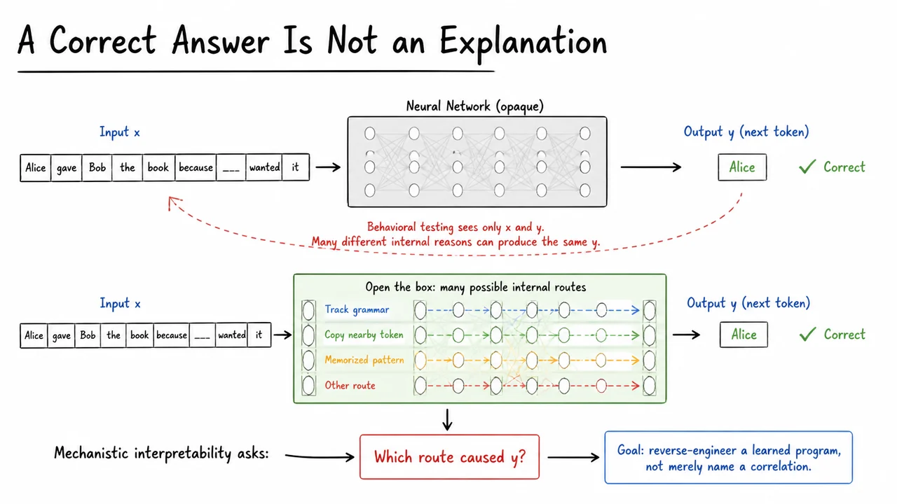
Take a simple completion: “Alice gave Bob the book because ___ wanted it.” Suppose the model assigns a high target logit $y$ to the correct next token. From the outside, this looks like success. But the same success could come from very different internal procedures. The model might track syntactic roles, exploit a memorized phrase pattern, copy a nearby name, or combine several weak heuristics. Observing the input sequence $x$ and the output $y$ does not tell us which of those stories is true.

That ambiguity is the starting point for mechanistic interpretability. A neural network is trained end to end, so its internal organization is not handed to us as readable source code. Yet the network still performs a sequence of computations between $x$ and $y$. If we want to understand the mechanism, we need to recover enough of those internal variables and transformations to explain why this particular output changed when the input changed.

The distinction matters because a behavioral description can be correct while remaining mechanistically empty. Saying “the model understands pronouns” summarizes a pattern of outputs. It does not identify where the relevant information appears internally, how it is moved between token positions, which components transform it, or whether removing those components would change $y$. A mechanistic explanation asks for those missing links.

A useful standard is predictive. If we claim that one internal pathway is responsible for the answer, then changing that pathway in a controlled way should change $y$ in a way our explanation anticipates. That turns interpretation from storytelling into an experimental science of internal cause and effect. The goal is not to find a pleasing label for an activation. It is to reverse-engineer a learned program well enough that its behavior under intervention becomes less mysterious.

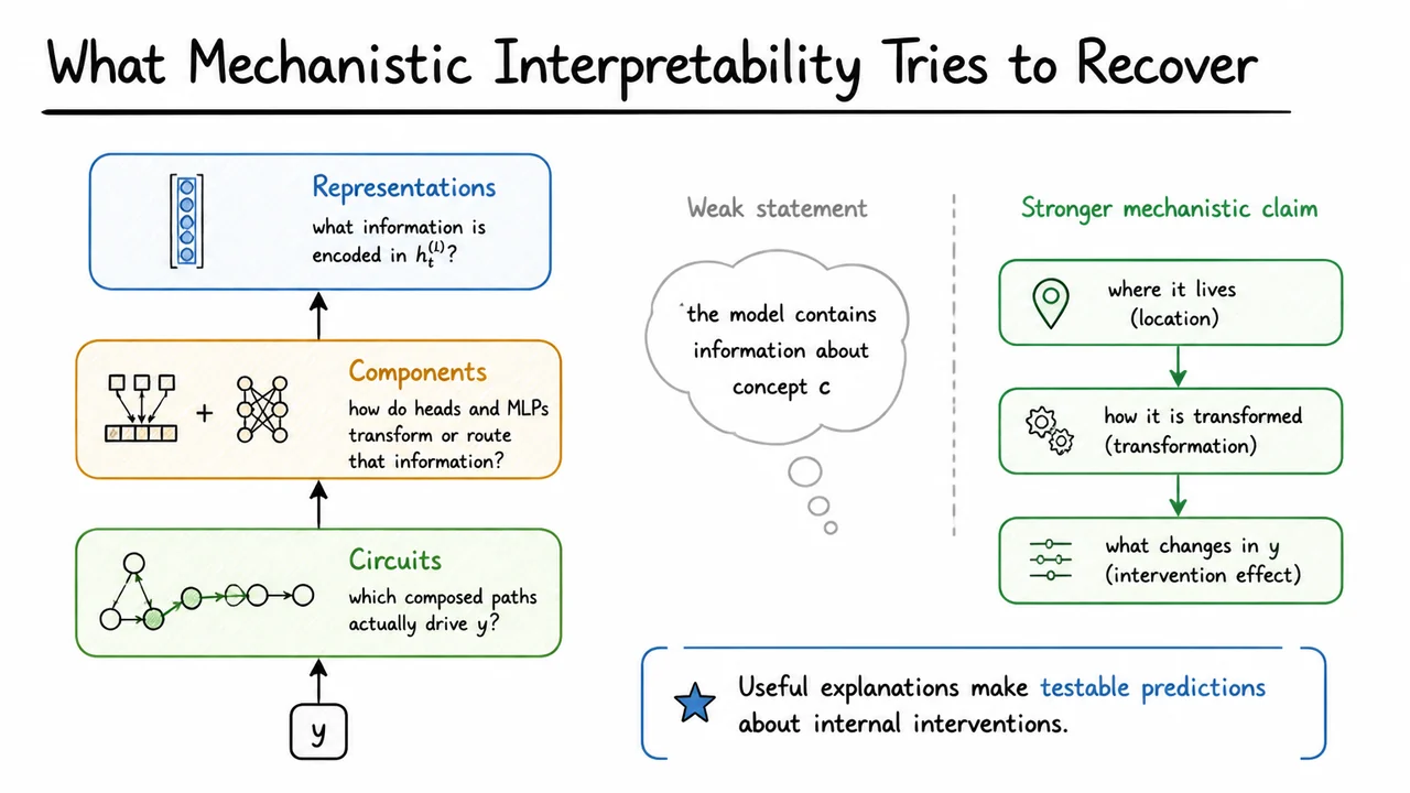
To make that goal precise, it helps to separate three levels of explanation.

The first level is representation. At some token position $t$ and layer $l$, the model carries an activation vector $h_t^{(l)}$. We can ask what information is present in that vector: perhaps the identity of an earlier token, whether a noun is singular, or whether the current context resembles a repeated pattern. This is already more specific than saying the model “knows” something, but it still leaves open whether the model actually uses that information.

The second level is component computation. Attention heads and MLPs read from the residual stream and write new information back into it. Here the question changes from “what is encoded?” to “what transformation is being performed?” A head may preferentially read from a previous matching token; an MLP may amplify a feature or combine several features. The important point is that the component has an operational role, not merely an associated semantic label.

The third level is a circuit: a composed path through several components that produces a behavior. A circuit explanation connects an upstream representation to one or more transformations and then to the analyzed output $y$. It tells us how information gets from where it is represented to where it matters.

This hierarchy also clarifies why probing alone is insufficient. If a learned probe $g$ can map an internal activation $A$ to a concept prediction $\hat{c}$, then the concept $c$ is decodable from $A$. But decodability does not show that the network's own computation uses that information. A strong mechanistic claim therefore combines localization with intervention: change the proposed representation or pathway and measure what happens to $y$.

The field is ultimately trying to recover a causal description of the model's internal computation: what is represented, which components manipulate it, and which interactions are responsible for the behavior we care about.

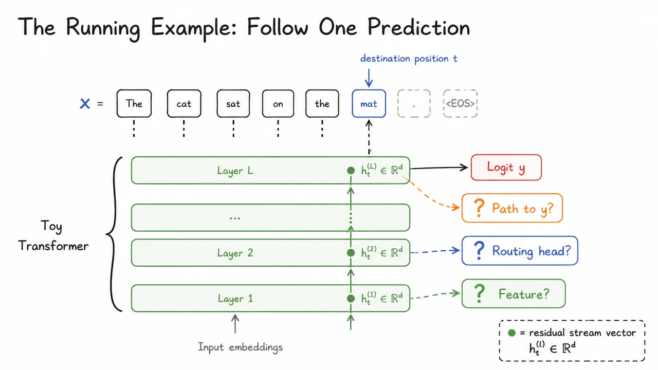
We will keep one concrete target in view. Consider a short input sequence $x$, and focus on the destination position $t$ where the transformer must choose its next token. Let $y$ denote the particular target logit we want to explain. Instead of treating the transformer as one giant function, imagine following the information available at position $t$ as it passes through the network.

After layer $l$, the residual stream at that position is a vector $h_t^{(l)}$ in a $d$-dimensional space:

$$h_t^{(l)} \in \mathbb{R}^d.$$

The vector is not a human-readable record. It is a learned state that many attention heads and MLPs can read and modify. Our job is to infer which directions or structures inside that state carry information relevant to the prediction.

For the running example, three questions organize the investigation. First, is there some internal feature that marks the earlier token or relation that matters for the completion? Second, does an attention head route that information from one token position to another? Third, which downstream pathway converts that routed signal into a change in the target logit $y$?

Notice what we are deliberately not doing yet. We are not declaring that a particular neuron means “Bob,” that an attention head “does pronouns,” or that a visually striking pattern is the mechanism. Those are hypotheses. They become useful only when they survive tests that distinguish correlation from causal contribution.

This running example gives us a small enough problem to reason about while preserving the structure of real interpretability work. The same workflow scales conceptually to more complicated behaviors: identify candidate representations, locate components that transform them, then intervene on the proposed path and see whether the output changes as predicted.

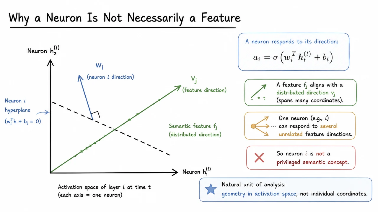
A natural first move is to inspect individual neurons. If neuron $i$ activates strongly whenever a certain concept appears, it is tempting to call that unit “the concept neuron.” The geometry of neural activations makes that interpretation much less secure than it sounds.

A typical neuron computes something like

$$a_i = \sigma(w_i^T h_t^{(l)} + b_i),$$

where $w_i$ is the neuron's incoming weight direction, $b_i$ is its bias, and $\sigma$ is a nonlinearity. Before the nonlinearity, the neuron is effectively measuring how far the activation vector points along a particular direction. That coordinate does not have any privileged semantic status merely because it belongs to one neuron.

A meaningful feature $f_j$ can instead be represented along some direction $v_j$ that cuts across many neuron coordinates. In that case, no single neuron cleanly corresponds to the feature. Conversely, one neuron axis can intersect several meaningful feature directions, so the same neuron may activate for apparently unrelated concepts. This phenomenon is often called polysemanticity.

The shift in perspective is important. Rather than asking only “which neuron fires?”, we can ask “which direction or subspace of activation space carries the relevant information?” That geometric view is better matched to how linear transformations inside transformers operate: matrices naturally read and write combinations of coordinates, not human-selected neurons.

This does not mean neuron-level analysis is useless. Some neurons can be unusually interpretable, and sparse structures can make individual units informative. The point is narrower: one-neuron-one-feature is an assumption that must be demonstrated, not a default. Once we stop insisting that semantic features align with coordinate axes, another possibility appears: perhaps the network can pack more meaningful features into its activation space than there are dimensions.

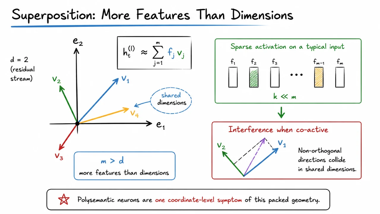
Suppose the residual stream approximately represents an activation as a combination of feature directions:

$$h_t^{(l)} \approx \sum_{j=1}^{m} f_j v_j.$$

Here $v_j$ is the direction associated with feature $j$, and $f_j$ is how strongly that feature is present. If every feature needed its own perfectly orthogonal direction, we could cleanly fit at most about $d$ independent directions into a $d$-dimensional residual stream. But neural networks often operate in sparse regimes: only a small subset of potentially relevant features is active on any one input.

That changes the packing problem. If only $k$ features are typically active and $k \ll m$, then the model can reuse dimensions by assigning features to non-orthogonal directions. In principle, this allows $m$ to exceed $d$. The representation is then in superposition: many possible features share the same underlying coordinates.

The benefit is capacity. A model can represent a large vocabulary of rare or context-specific features without dedicating one axis to each one. The cost is interference. If two non-orthogonal features are active at the same time, the vector contribution from one can contaminate a readout aligned with the other.

This explains why polysemanticity should not be surprising. A neuron coordinate is simply one axis through the packed activation space. If several feature directions cross that axis, the neuron may participate in representing several unrelated concepts.

Superposition is best viewed as a representational tradeoff, not a pathology by definition. The network may accept some interference because sparsity keeps most collisions manageable. For interpretability, however, the consequence is substantial: the native neuron basis can be a poor basis for human-readable concepts. We may need methods that recover the hidden feature directions themselves rather than interpreting raw coordinates one by one.

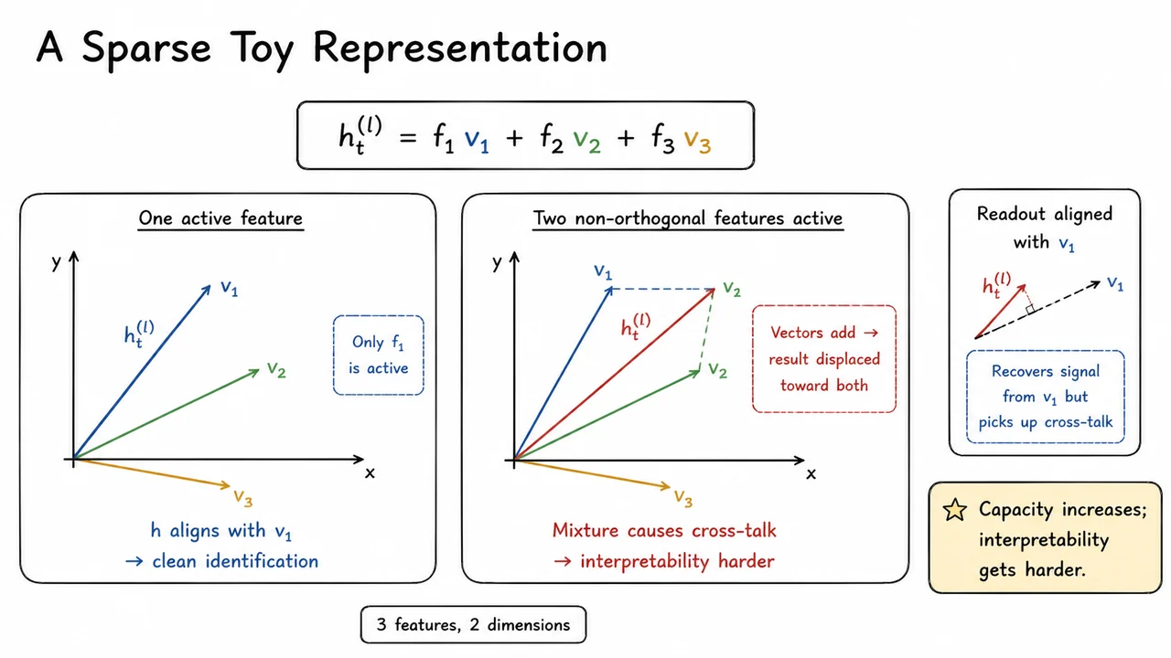
A two-dimensional toy example makes the superposition tradeoff concrete. Imagine three feature directions $v_1$, $v_2$, and $v_3$ packed into only two dimensions. The activation is

$$h_t^{(l)} = f_1v_1 + f_2v_2 + f_3v_3.$$

If only one feature is active, say $f_1$ is nonzero while the others vanish, then $h_t^{(l)}$ points directly along $v_1$. A readout aligned with $v_1$ can identify that feature cleanly even though the space contains three candidate features in only two dimensions.

Now let two non-orthogonal features activate together. Their contributions add as vectors, so the resulting $h_t^{(l)}$ points somewhere between the two feature directions. A readout aligned with $v_1$ still sees a strong signal from feature 1, but it may also pick up a contribution from feature 2 because $v_1$ and $v_2$ are not orthogonal. That is the interference cost of packing.

The example clarifies an important distinction. The representation can be useful for the model even when it is awkward for us. Downstream learned matrices can exploit the geometry statistically, tolerating some cross-talk because the relevant co-activations are rare or predictable. Human interpreters, however, would prefer a basis in which each meaningful feature is isolated.

This is why methods for feature discovery are attractive. They attempt to infer directions that correspond more closely to the sparse latent variables the network appears to use. But before we reach those methods, we need to understand how represented information becomes computation. In transformers, attention gives us a particularly clean local mechanism: one position can decide where to read from and what information to copy.

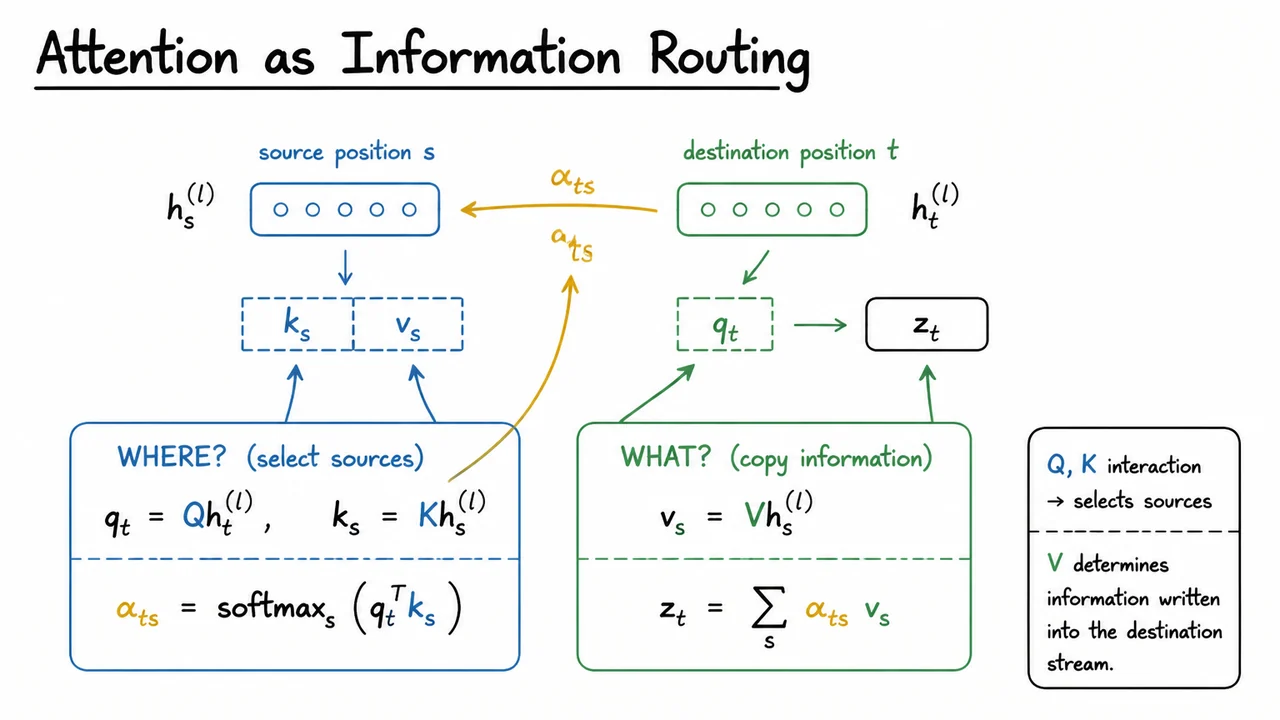
Consider one attention head operating at destination position $t$. The head first forms a query from the current residual state and keys from possible source positions:

$$q_t = Qh_t^{(l)}, \qquad k_s = Kh_s^{(l)}.$$

The query-key similarity determines how strongly position $t$ attends to source position $s$:

$$\alpha_{ts} = \operatorname{softmax}_s(q_t^T k_s).$$

This part of the computation answers a routing question: where should the head read from? If the current destination state contains a feature that matches a feature encoded at some earlier position, the learned $Q$ and $K$ matrices can make the corresponding dot product large.

The head then computes a value vector from each source:

$$v_s = Vh_s^{(l)},$$

and combines those values using the attention weights:

$$z_t = \sum_s \alpha_{ts}v_s.$$

This second part answers a different question: what information should be copied from the selected source? The value map $V$ can extract a feature from the source state, while the attention pattern controls where that feature comes from.

That separation is useful for mechanistic reasoning. A head can be understood as a routing primitive whose selection behavior and copied content are analyzed separately. An attention pattern by itself is therefore incomplete evidence. Two heads can attend to the same position while writing very different information into the residual stream.

In the running example, we might hypothesize that a destination position contains a query-like feature that causes the head to look back toward a relevant earlier token. The next question is whether such routing can implement a recognizable algorithm rather than a one-off lookup. Induction heads provide a canonical case.

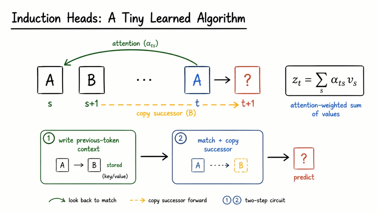
Take a repeated sequence pattern such as A B ... A. At the second occurrence of A, a useful continuation rule is: find an earlier matching A, then predict whatever followed it before, namely B. This is the core intuition behind induction-style behavior.

Mechanistically, the later position needs information that lets its query match a representation associated with the earlier context. When that match is strong, the attention weight $\alpha_{ts}$ concentrates on the useful source position $s$. The head then copies information through

$$z_t = \sum_s \alpha_{ts}v_s.$$

If the selected value carries a signal favoring the token that followed the earlier match, the downstream model can use that signal to raise the corresponding next-token logit.

A common circuit picture is two-step. An upstream component first writes previous-token information into the residual stream, so a position can represent something about its predecessor. A later induction head then matches the current context against that stored pattern and retrieves information about the earlier successor. The behavior therefore emerges from interaction between multiple components rather than from one magically self-contained head.

This example is useful because it shows what a mechanistic explanation can look like. We do not merely say that a head “attends backward.” We specify what feature makes the match happen, what information is present in the selected value, and how the copied signal changes the prediction.

The exact implementation can vary across models and contexts, so “induction head” should not become a substitute for analysis. The larger lesson is that transformer components can compose into small learned algorithms. That naturally leads from interpreting isolated heads to interpreting circuits.

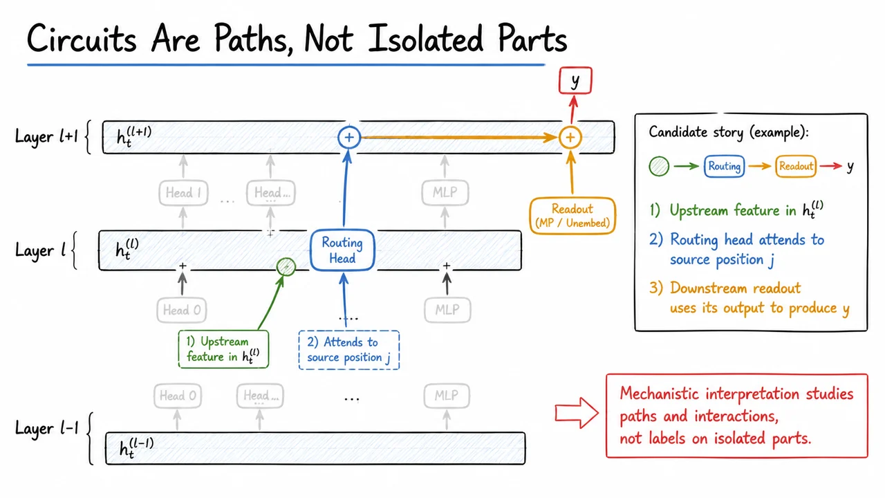
A transformer repeatedly adds the outputs of attention heads and MLPs into the residual stream. Because many components read from the same evolving state, the functional meaning of one component depends on what information arrives upstream and where its output is used downstream.

This is why a circuit is better thought of as a selected computational subgraph than as a collection of individually interesting parts. Suppose an upstream feature in $h_t^{(l)}$ causes one head to route information from a relevant token. A downstream component may then read that routed feature and convert it into a contribution that changes the target logit $y$. The explanatory object is the whole path: feature, routing operation, downstream readout, output effect.

A head can look striking in isolation yet be irrelevant to the behavior we care about. Conversely, a modest-looking component can be crucial because it supplies exactly the feature a downstream component needs. Circuit analysis therefore asks about interactions and information flow, not just salience.

The residual stream makes this compositional view especially natural. Components effectively write contributions into a shared workspace, and later components can combine those contributions. That means causal influence may be distributed across several parallel or sequential routes.

For the running example, a candidate circuit might begin with a feature that identifies the relevant earlier token, pass through an attention head that copies that information to the destination position, and terminate in a downstream computation that increases $y$. But a diagram of that story is only a hypothesis. To know whether the path actually matters, we need tools that distinguish “this activation is associated with the answer” from “changing this activation changes the answer.”

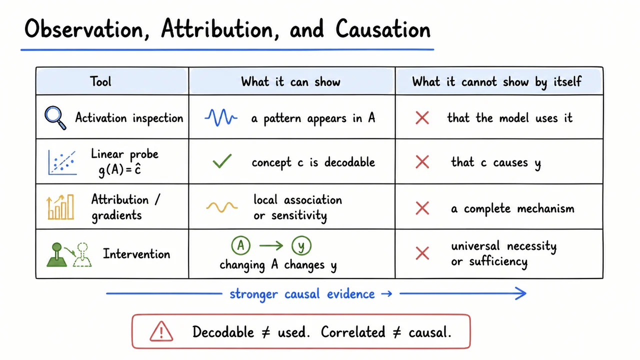
Interpretability tools differ mainly in the strength of claim they support. Activation inspection is the weakest form: we observe that some internal state $A$ behaves differently across inputs. That can reveal structure, but it does not establish that the model uses the structure to produce $y$.

A linear probe strengthens the descriptive claim. If a learned map $g$ predicts a concept label $\hat{c}$ from $A$, then information about concept $c$ is decodable from that activation. This can be valuable for localization. Yet a sufficiently expressive or data-rich probe may extract information that is present but irrelevant to the model's own computation.

Attribution and gradient methods ask how changes in internal quantities are associated with or locally influence the output. They can help prioritize components, but they usually do not by themselves identify a complete causal mechanism.

Causal interventions go further because they directly modify the network's internal state and measure the resulting change in $y$. If replacing or ablating $A$ systematically changes the target output, we have stronger evidence that $A$ participates in the behavior.

Even interventions need careful interpretation. A particular replacement might push the model into an unusual internal state, or a redundant pathway might compensate for the one we removed. So causal evidence is not a binary stamp of truth. It is stronger evidence tied to a specific counterfactual.

A useful hierarchy is therefore: observation tells us where to look; probes tell us what can be decoded; attribution tells us which quantities may matter; interventions test whether the proposed internal information is actually used. Mechanistic claims should match the evidential strength of the tool.

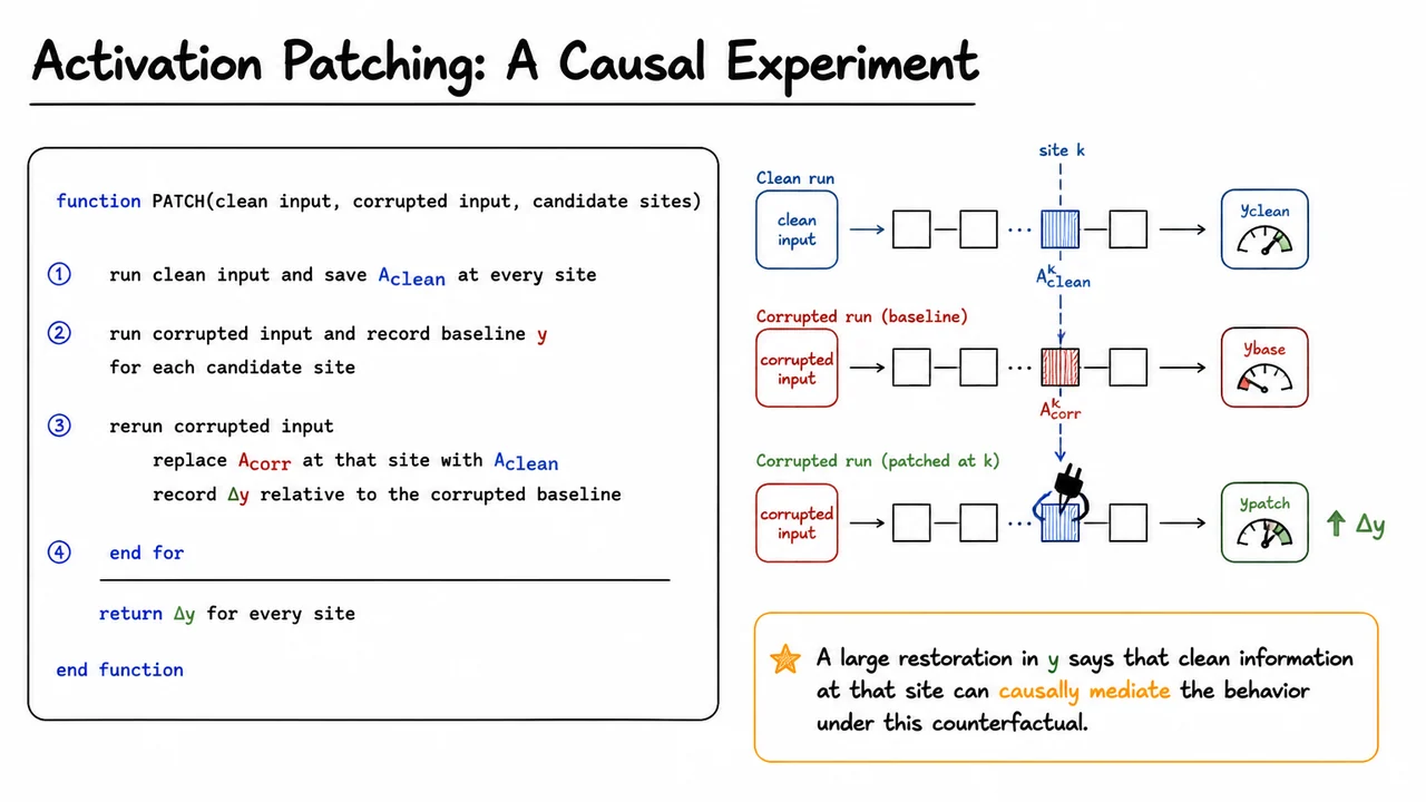
Activation patching is a direct way to test whether information at a particular internal site causally mediates a behavior. Start with two related inputs: a clean input that produces the behavior of interest, and a corrupted input designed to weaken or change that behavior.

Run the clean input and save the activation $A_{clean}$ at candidate sites. Then run the corrupted input and record its baseline output $y$. For one candidate site at a time, rerun the corrupted input but replace its activation $A_{corr}$ with the clean activation $A_{clean}$. Measure the resulting change $\Delta y$ relative to the corrupted baseline.

Conceptually, the procedure is:

1. Record clean activations.
2. Record the corrupted baseline.
3. Patch one clean activation into the corrupted run.
4. Measure how much the target output recovers.
5. Repeat across candidate sites.

If patching one site produces a large restoration in $y$, that is evidence that the clean information present there can causally mediate the behavior under this counterfactual. In our running example, we might corrupt the earlier token relation, then ask whether inserting the clean activation at a particular head or residual-stream location restores the correct next-token logit.

The phrase “under this counterfactual” matters. Patching does not prove that the site is universally necessary, nor that the activation has one simple semantic meaning. It tells us that transplanting clean information into that location changes the downstream computation in a predicted direction.

This makes activation patching especially useful for circuit discovery. A broad scan can localize layers, positions, or components whose clean states restore behavior. More targeted experiments can then test specific pathways and refine the causal story.

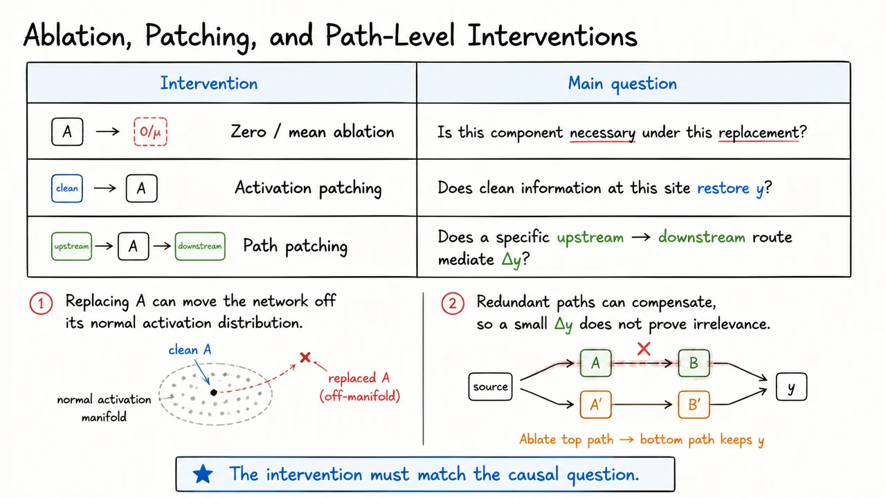
Several intervention methods look similar on the surface but answer different causal questions.

With ablation, we replace or remove a component's activation, often by setting it to zero or to some reference such as a mean activation. If $y$ changes substantially, the component appears necessary under that replacement. But the replacement itself matters: zero may be far outside the activation distribution the model normally encounters.

With activation patching, we replace $A_{corr}$ with $A_{clean}$ and ask whether clean information at that site restores the behavior. This is a mediation-style question: does this location carry something that can rescue the target output?

With path-level interventions, we try to isolate a particular upstream-to-downstream route. The goal is to ask whether a specific connection mediates the observed $\Delta y$, rather than merely whether one node matters somewhere in the network.

Two complications recur across all three methods. First, interventions can create distribution shift. A highly unnatural activation may cause downstream components to behave strangely, so the measured effect partly reflects the intervention artifact. Second, neural networks can contain redundancy. If two routes can carry similar information, ablating either one alone may produce a small effect even though the information is essential collectively.

For that reason, intervention results should be interpreted in relation to the exact replacement and the exact causal question. A small $\Delta y$ is not proof of irrelevance, and a large $\Delta y$ does not automatically identify a unique mechanism.

The practical lesson is to design a family of counterfactuals rather than relying on one dramatic ablation. Mechanistic confidence grows when several interventions tell a consistent story about the same proposed pathway.

Superposition gives us a reason to search for a better basis than the model's native neuron coordinates. Sparse autoencoders, or SAEs, attempt to learn such a basis from activation data.

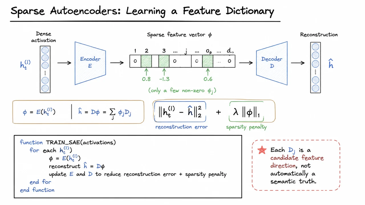
Given a residual-stream activation $h_t^{(l)}$, an encoder $E$ maps it to a set of feature activations. We can write the encoded features collectively as $\phi$, with individual feature activation $\phi_j$. A decoder matrix $D$ reconstructs the original activation:

$$\phi = E(h_t^{(l)}),$$

$$\hat{h} = D\phi = \sum_j \phi_jD_j.$$

The decoder direction $D_j$ is then treated as a candidate feature direction. To encourage the representation to use only a small number of features at once, training combines reconstruction accuracy with a sparsity penalty:

$$\|h_t^{(l)}-\hat{h}\|_2^2 + \lambda\|\phi\|_1.$$

The first term asks the autoencoder to preserve the information in the original activation. The second discourages many features from firing simultaneously. If the tradeoff works well, the SAE can turn a dense, polysemantic activation into a sparser set of directions that are easier to inspect.

This can be extremely useful for mechanistic work, but the learned features should not be treated as ground truth concepts. One human concept may split across several SAE features, or one learned feature may combine several patterns. Different training choices can also produce different dictionaries.

So SAE interpretation is a hypothesis-generation step. We inspect which inputs activate $\phi_j$, infer a possible meaning for $D_j$, and then ask whether manipulating that feature changes downstream behavior. The same causal standard still applies: readable features are valuable, but mechanistic understanding requires evidence that the model actually uses them.

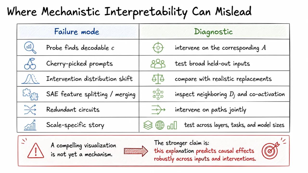
Mechanistic interpretability is unusually vulnerable to convincing stories. A heatmap can look structured, a probe can achieve high accuracy, and an SAE feature can have a memorable label. None of those observations alone guarantees that we have identified the mechanism.

A probe can succeed because information about $c$ is present in $A$ even if the model never uses that information. The diagnostic is to intervene on the relevant internal representation and measure the effect on $y$.

Prompt selection can also mislead. If a circuit is demonstrated only on a handful of carefully chosen examples, the explanation may capture a local pattern rather than a robust computation. Testing broad held-out inputs reveals whether the proposed mechanism generalizes.

Interventions bring their own failure modes. Replacing an activation with zero can push the network off its normal internal distribution. Redundant pathways can hide importance because removing one route leaves another intact. Path-level or joint interventions can help distinguish redundancy from irrelevance.

Sparse autoencoders introduce another layer of ambiguity. A single semantic concept may be split across several decoder directions $D_j$, while one learned feature may merge multiple patterns. Inspecting neighboring features, co-activation structure, and causal effects is therefore more informative than attaching one label and stopping.

Scale can change the story as well. A mechanism found in one layer, task, or model size may reorganize elsewhere. Strong claims should survive variation across inputs and, when possible, across related settings.

The recurring standard is simple: a mechanistic explanation should do more than fit observations after the fact. It should predict what targeted internal changes will do, and those predictions should remain reasonably stable across the conditions where we claim the explanation applies.

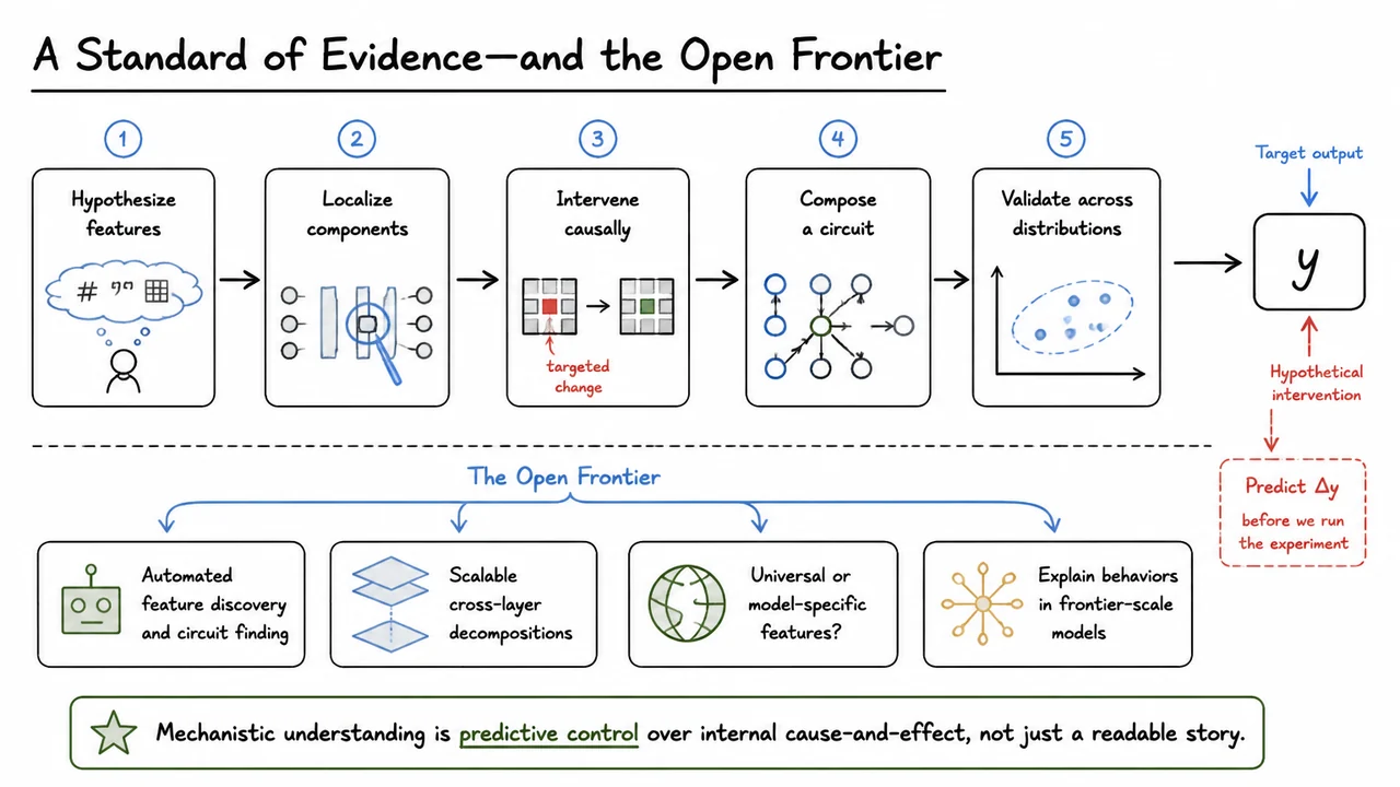
The pieces now fit into a disciplined workflow.

First, propose candidate features that might explain the behavior. Second, localize the components that read, transform, or route those features. Third, intervene on the relevant activations and measure changes in the target output $y$. Fourth, compose the validated pieces into a circuit rather than treating each component in isolation. Finally, test the explanation across inputs and counterfactuals that were not used to construct it.

That workflow turns the opening question into something operational. If we claim that a particular internal path causes the model's prediction, we should be able to forecast the effect of changing that path before we run the experiment. When the forecast succeeds repeatedly, the explanation begins to resemble reverse engineering rather than retrospective storytelling.

The open frontier is largely about scale and automation. Researchers want methods that discover useful features automatically, identify circuits without hand-inspecting thousands of components, and decompose computation across layers rather than one activation site at a time. Sparse feature methods and cross-layer decompositions are attempts in that direction.

Another open question is universality. Do different models learn similar internal features and circuits because the task demands them, or does each model invent a substantially different representation? The answer matters if we hope to build reusable interpretability tools rather than one-off analyses.

Most importantly, frontier-scale systems force a sharper standard of evidence. A readable feature name is not enough, and a single successful ablation is not enough. The strongest form of mechanistic understanding is predictive control over internal cause and effect: we know enough about the learned computation to say what an internal edit should do to $y$, then observe the predicted consequence.

That standard is demanding, but it is exactly what makes mechanistic interpretability different from merely visualizing a neural network. The ambition is to recover the algorithms hidden inside the learned weights well enough that their behavior becomes experimentally testable.