When we first learn reinforcement learning, it is tempting to imagine that the hardest part is estimating a good value function and then simply acting greedily with respect to it. That works beautifully in discrete problems with a small action set: learn , choose , and you have a policy. The logic is elegant because it reduces control to prediction.
But that elegance hides an important assumption: that the action space is easy to search, that one action is enough to represent the right behavior, and that the agent can truly observe the relevant state. Once any of those assumptions breaks, a value function alone becomes a brittle intermediary rather than a solution.
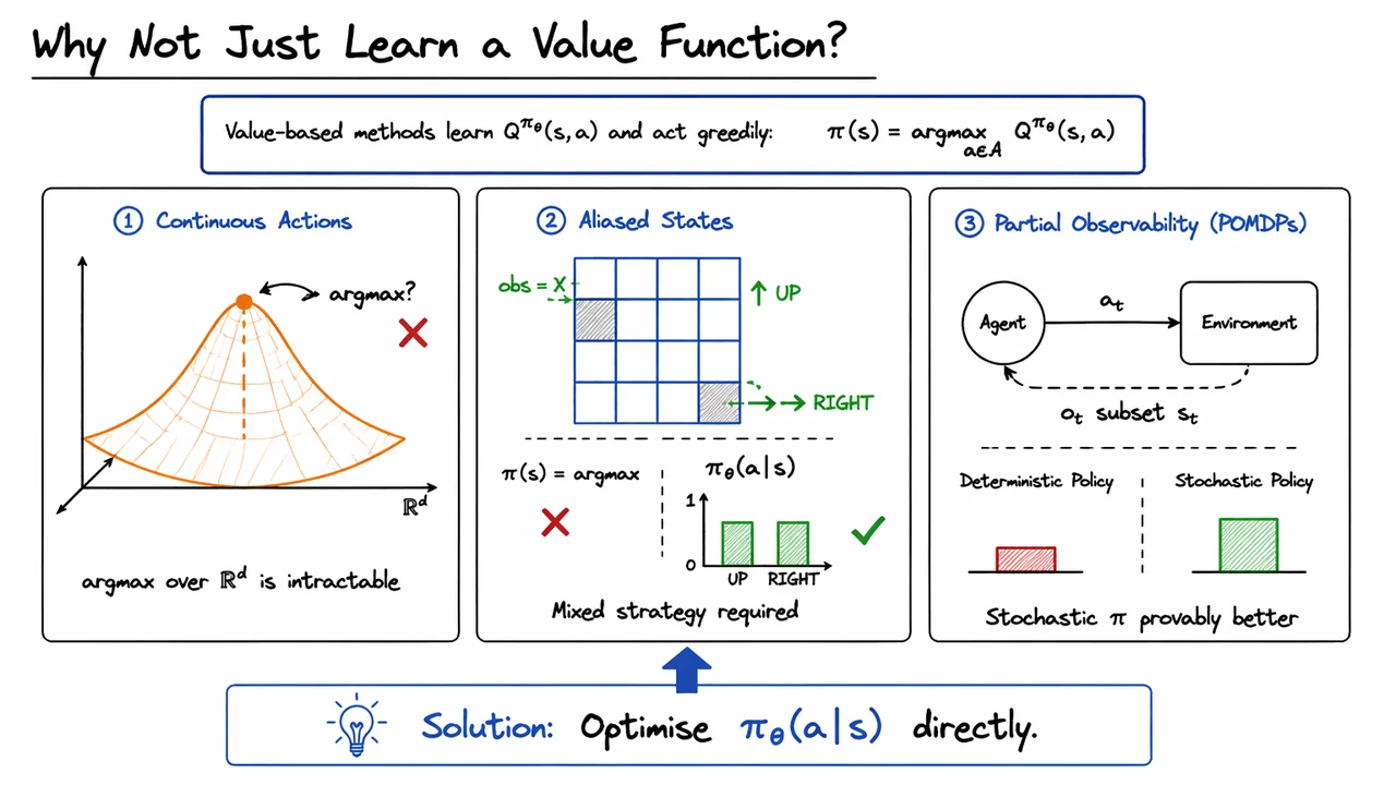
The greedy policy induced by a value function is typically written as This expression is harmless when is finite and small. In that case, the argmax is just a comparison over a short list. But if , the expression quietly becomes a nested optimisation problem: every time the agent wants to act, it must solve a continuous maximisation over actions. For high-dimensional control, that is not a small implementation detail — it is the central computational bottleneck.
That is the first failure mode: continuous actions. Here, the issue is not that -learning is conceptually wrong, but that the greedy extraction step is no longer cheap. We are no longer choosing among a handful of actions; we are searching over an uncountable space. Unless the critic has a special structure, is itself a hard optimisation problem, and we have merely moved the difficulty from policy learning into action selection.
The second failure mode is more subtle: perceptual aliasing. Imagine two different underlying situations that produce the same observation. From the agent’s perspective, the states are indistinguishable, but the correct behavior may differ. A deterministic greedy policy must commit to one action per observation, yet the best response may require a mixture over actions. In that case, the policy needs to encode uncertainty or ambiguity directly: A stochastic policy can represent “sometimes go left, sometimes go right” in a principled way; a pure argmax policy cannot.
This distinction matters because the right response is not always “pick the single best action.” When two hidden states collapse to the same observation, the agent may need to randomize to average over incompatible optimal actions. In other words, the policy is not just a decision rule; it is part of the model of how the agent resolves ambiguity.
The third failure mode is partial observability, where the agent does not directly observe the full Markov state at all. In a POMDP, the observation history or belief state is what matters, and deterministic policies can be fundamentally suboptimal. Stochasticity is not merely a convenience here — it can be structurally necessary, and there are settings where the best deterministic policy performs arbitrarily badly compared with a stochastic one. This is one of the most important conceptual reasons to stop treating “policy = argmax over value” as the universal template.
So the real lesson is not “value functions are useless.” Rather, value functions are often the wrong interface for control. If the action space is large or continuous, or if the environment forces the agent to randomize, then the policy itself should be optimized directly. That is exactly what policy gradient methods do: instead of first learning a value surface and then extracting a policy by maximization, we parameterize the policy and improve by following the gradient of expected return.
The visual below compresses these three failure modes into one glance. The left panel emphasizes that in continuous action spaces, the obstacle is the search problem hidden inside . The middle panel shows why aliased observations can demand a mixed strategy, making a stochastic policy strictly more expressive than a deterministic one. The right panel captures the POMDP intuition: when the agent does not fully observe the state, stochastic policies can outperform any fixed deterministic rule.
Taken together, the three panels justify the move that policy gradient methods make from the start: rather than asking how to recover a policy from a value function, we ask how to optimize the policy directly. That shift is what makes the rest of the lecture possible — from the likelihood-ratio derivation to REINFORCE, baselines, and actor-critic methods.
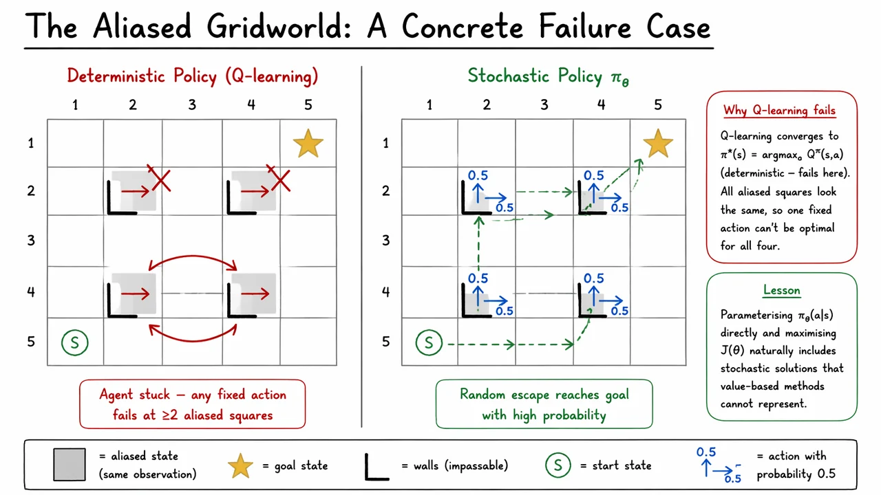
We now want a failure case that is simple enough to reason about in one glance, but rich enough to expose the real limitation of value-based control. The key idea is perceptual aliasing: the environment may be fully Markov in the underlying state, yet the agent’s observation collapses several distinct states into the same feature vector. Once that happens, the policy no longer gets to condition on the true state, only on what it can see.
That distinction matters because a value method such as Q-learning ultimately extracts a deterministic control rule, so every observation is mapped to a single action. If two or more hidden states share the same observation but require different actions, then a deterministic policy is forced to “average over” incompatible choices by committing to one of them. In a standard MDP with full observability, that is usually fine; in an aliased setting, it can be fatal.
A small gridworld makes the issue concrete. Imagine a grid with a goal in one corner and four interior squares that all look identical locally: each has walls on the same two sides, so the agent sees the same feature vector in all four places. The true state differs, but the observation does not. From the agent’s perspective, these are not four distinct situations — they are one ambiguous observation repeated in four locations.
Now ask what a deterministic policy can do. Because it must output a single action for the shared observation, it must choose the same move in each aliased square. But no single move is simultaneously correct everywhere: an action that escapes one hidden configuration may hit a wall or send the agent into a loop in another. In this kind of construction, any fixed choice incurs a substantial failure probability, and the expected return stays low. The problem is not that the policy is poorly trained; the problem is that the policy class is too rigid.
A stochastic policy is different in exactly the right way. Instead of collapsing the decision to one action, it can represent a distribution or symmetrically over , so that the agent randomizes between two perpendicular escape directions. This is not indecision for its own sake; it is a principled response to partial observability. When the same observation corresponds to several hidden states, randomization can hedge against the hidden ambiguity and produce a much higher return than any deterministic commitment.
This is exactly why the usual greedy value-based view can break down here. The maximizer assumes that one action should dominate for the state under consideration. But when the observation aliases multiple hidden states, the induced greedy policy is still deterministic and therefore cannot adapt to each hidden case separately. Even if the Q-function is accurate with respect to the underlying hidden dynamics, the final policy extraction step throws away the very stochasticity that would solve the task.
The broader lesson is that we should optimize the policy directly, not merely infer it indirectly from values. By parameterizing and maximizing , we allow the model class itself to include useful stochastic strategies. That is the real motivation for policy gradients: they are not just another way to train controllers, but a way to learn policies whose distributional structure is essential to success.
The visual below compresses this argument into two contrasted worlds. On the left, the deterministic controller is trapped by a single committed action: the same red arrow must serve every aliased square, so at least some hidden cases fail or cycle. On the right, the stochastic policy assigns probability mass to multiple actions, and that extra flexibility lets the agent escape the ambiguous region and reach the goal with high probability.
If you keep one idea from this example, let it be this: when the observation is ambiguous, the right object to learn is not just a value function, but a parameterized policy distribution. This is the conceptual bridge from “why not just learn a value function?” to the policy-gradient objective that follows.
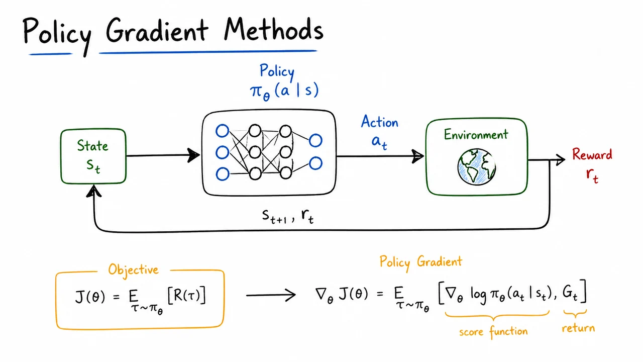
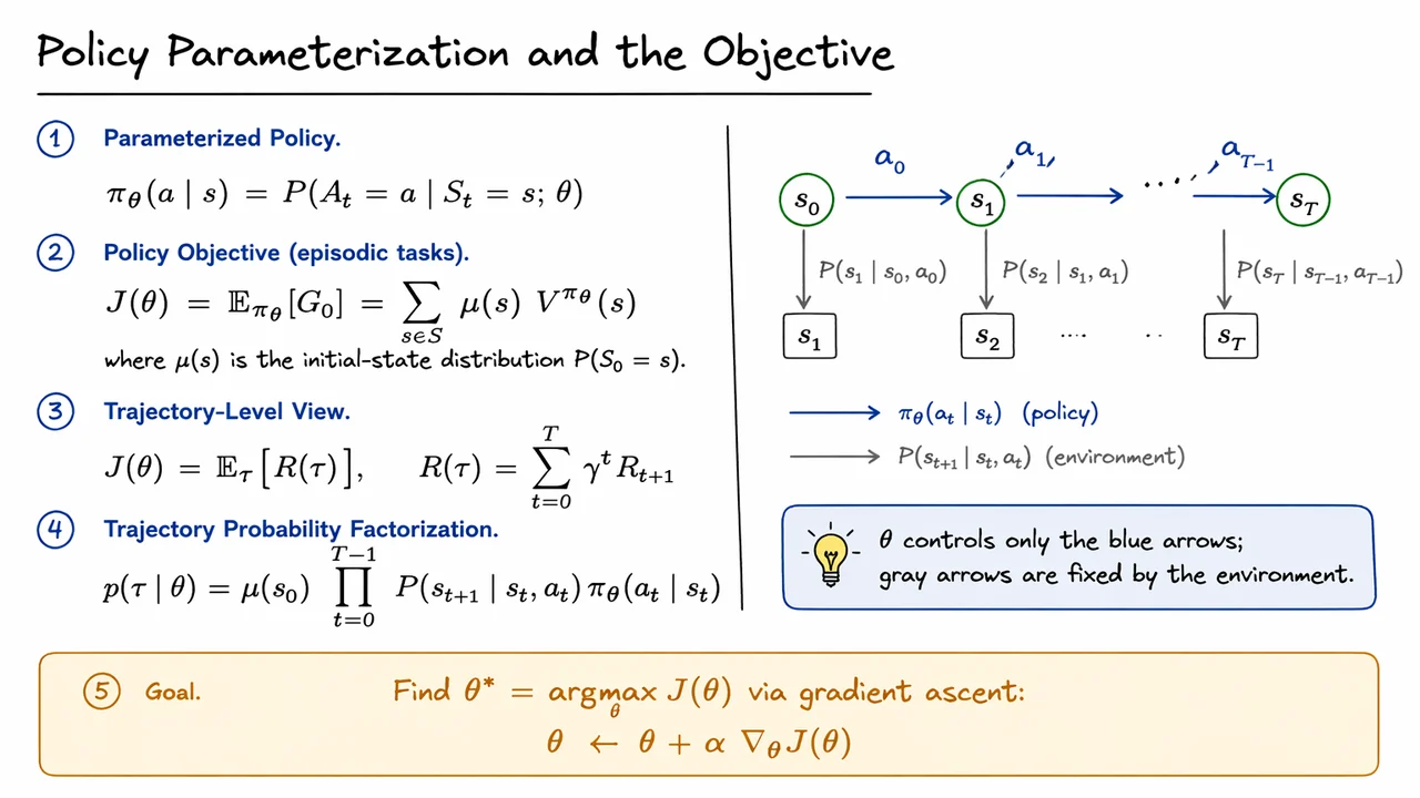
After the failure modes of aliasing, the next question is almost unavoidable: what exactly are we optimizing when we say “learn a policy”? In policy gradients, the answer is not a value table or a greedy action rule, but a parameterized stochastic policy whose parameters can be adjusted by gradient ascent. Formally, at each time , the policy defines a distribution over actions, so the policy is not a single action choice but a family of action probabilities that can be made sharper, smoother, or more exploratory depending on .
The objective in episodic reinforcement learning is to choose so that trajectories with high long-term return become more likely. A standard way to write this is where is the discounted return from the start of an episode. This is already useful conceptually: instead of optimizing immediate reward, we optimize the expected total outcome under the policy’s own behavior. If the initial state is random, we can also view this as an average over the initial-state distribution : This makes the dependence on the policy explicit through the value function , while separating it from the environment’s starting-state distribution.
It is often cleaner to reason not at the level of states, but at the level of entire trajectories. A trajectory is a full episode sampled from the policy and the environment dynamics, and the same objective can be written as This trajectory view is the one that later makes the likelihood-ratio trick work. It turns the objective into an expectation over a distribution , which is the key object we need when differentiating .
The crucial structural fact is that the trajectory probability factorizes into two very different parts: Only the policy terms depend on . The environment transition probabilities and the initial-state distribution are fixed by the environment. This distinction matters enormously: it is what makes policy gradients possible even when the dynamics are unknown, non-differentiable, or too complex to model directly. We never need to differentiate through the environment; we only need to know how the policy assigns probability to the actions it takes.
This also explains why policy-gradient methods are so different from value-based methods. Instead of solving for a greedy argmax over actions, we directly reshape the action distribution so that trajectories with larger return become more likely. In that sense, the optimization problem is:
That update rule is deceptively simple, because the real challenge is estimating from sampled experience. But once the objective has been written at the trajectory level, the path to REINFORCE and the policy gradient theorem becomes natural: we will differentiate an expectation over trajectories, isolate the -dependent policy factors, and turn return-weighted action probabilities into a usable learning signal.
The visual below compresses exactly that logic. The left side collects the same objective in three equivalent forms: policy, state-value, and trajectory expectation. That progression is not redundant; it shows that we can move between local decisions and global episode performance without changing the underlying quantity we optimize. The final boxed update rule at the bottom is there to remind you that all of this structure ultimately feeds one operation: gradient ascent on .
On the right, the unrolled trajectory diagram reinforces the most important modeling asymmetry: the blue arrows are controlled by , while the gray arrows belong to the environment. That is the conceptual hinge of policy gradients. We are not trying to redesign the world; we are only adjusting how the agent samples actions inside it.
After introducing the policy objective, the next question is not why we would optimize a stochastic policy, but how we can take gradients of it in a form that is actually usable. The key object is the score function : once this quantity is available, the policy gradient machinery becomes concrete, because the gradient of the return can be written as an expectation of that score weighted by advantage-like signals.
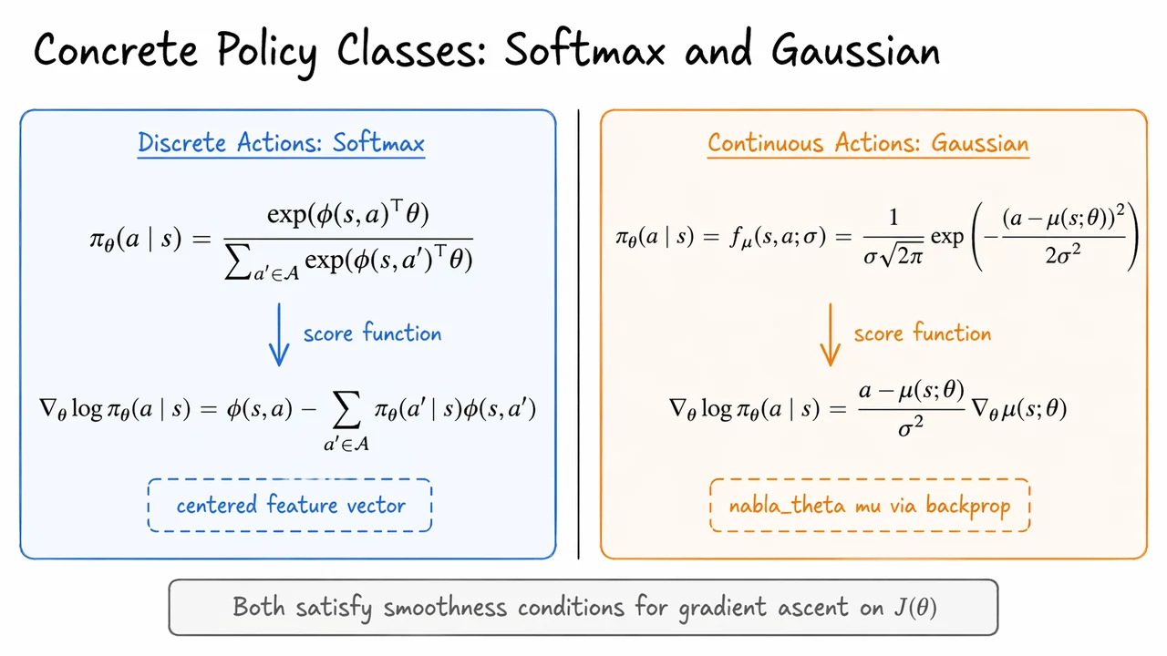
The point of this section is that two standard policy classes give us exactly the kind of differentiable structure we need. They look different—one for discrete action spaces, one for continuous action spaces—but both produce a clean log-derivative that can be computed by ordinary backpropagation. That is the crucial bridge between abstract policy optimization and implementable algorithms.
For a discrete action set, the most common choice is the softmax policy. If we assign each action a feature vector , then the policy is This is just a normalized exponential family model over actions: the numerator prefers actions whose features align with , and the denominator ensures the probabilities sum to one. The shape of the resulting gradient is especially elegant: In words, the update direction is the observed feature vector minus the policy’s own expected feature vector. That centering matters: it prevents the gradient from simply chasing large feature magnitudes and instead measures how surprising the chosen action was relative to the current policy. This is one reason softmax policies behave so naturally in REINFORCE-style updates.
For continuous actions, the canonical choice is a Gaussian policy. Instead of selecting an action from a finite set, the policy outputs a mean and samples around it: Here the policy class is smooth in the parameters through the mean network , and the score function becomes This expression is extremely informative. The scalar factor says that actions sampled above the mean and below the mean push the network in opposite directions, with larger deviations creating stronger learning signals. The vector factor is where standard backpropagation enters: once the mean is represented by a neural network, the policy gradient can be propagated through it exactly like any other differentiable model.
A useful way to compare the two cases is:
This smoothness is not a cosmetic detail. Policy gradient theory relies on being able to exchange differentiation and expectation, so the parameterization must be well-behaved enough for the gradient of to pass through the stochastic action selection. Softmax and Gaussian policies are the workhorses because they satisfy this requirement while still remaining simple enough to evaluate and differentiate exactly.
The visual below condenses that story into two parallel pipelines. The left panel captures the softmax case as “scores probabilities centered features,” while the right panel shows the Gaussian case as “mean network density backpropagated score.” Read together, they reinforce the main lesson: the policy gradient method does not need to differentiate through the sampling operation itself; it only needs a policy class whose log-derivative is tractable.
That is why these two parameterizations appear so early in the policy-gradient story. They are not merely convenient examples; they are the concrete templates from which REINFORCE, baseline methods, and actor-critic algorithms all inherit their gradient estimates.
Having defined a policy class, the next question is not what to optimize, but how to differentiate the objective efficiently. In policy gradient methods, we want to maximize
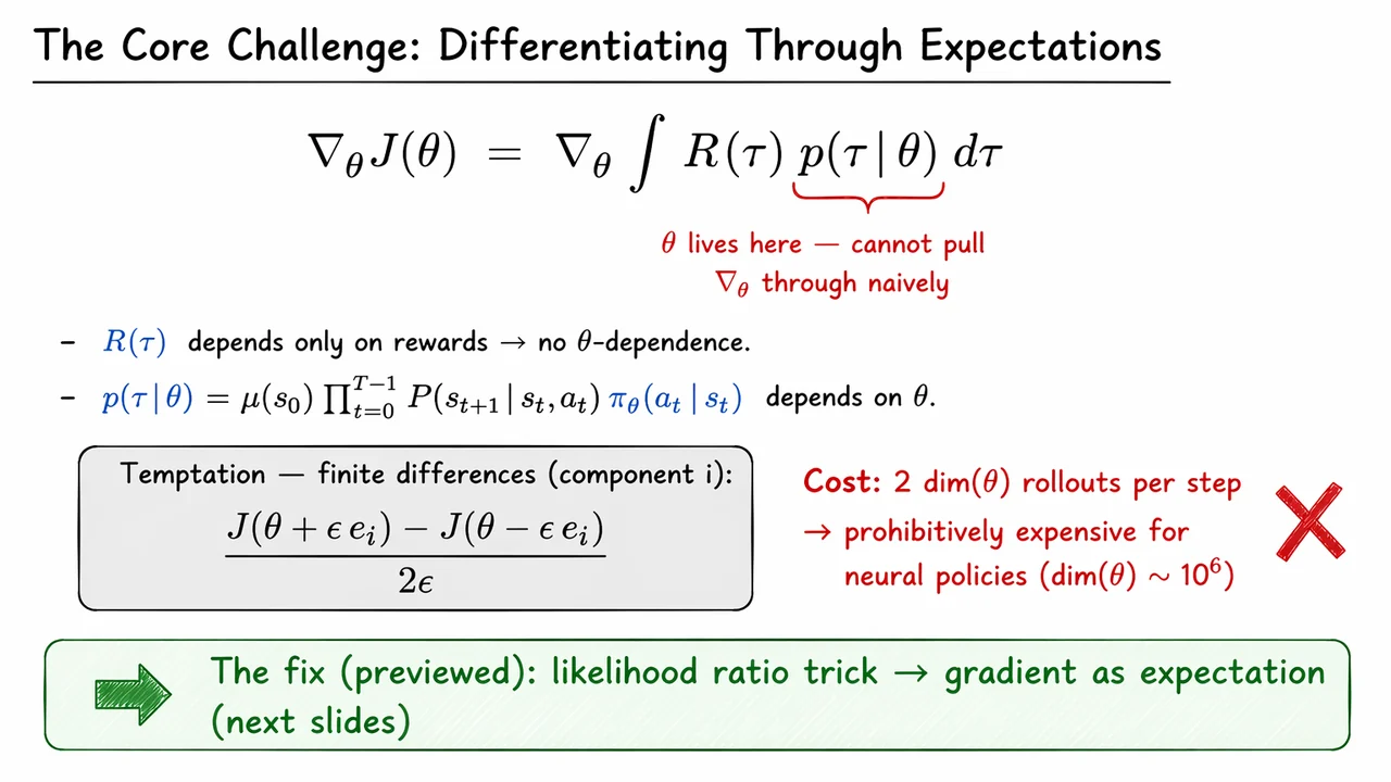
where denotes an entire trajectory and is the return accumulated along it. The key subtlety is that does not appear inside the reward function itself; it appears in the distribution over trajectories. That means the objective is an expectation whose measure depends on the parameters we are trying to optimize. This is exactly the kind of situation where naive differentiation becomes awkward.
If we write the gradient directly, we get
At first glance, this looks like something we might pass through the integral sign. But that instinct hides the real difficulty: the integrand is not just , it is times a parameter-dependent density. The domain of integration over trajectories does not move, but the probability mass assigned to each trajectory does. So the challenge is not “differentiate the reward”; it is “differentiate through the sampling distribution that generates the data.”
This distinction matters because in reinforcement learning, the return is often noisy, delayed, and discontinuous with respect to actions. There is usually no differentiable computational graph from to in the way that standard backpropagation assumes. Instead, the policy influences the likelihood of seeing different trajectories:
Here the environment dynamics and initial-state distribution are typically fixed, while the policy is the only factor that changes with . This is the source of the gradient signal—but also the source of the technical obstacle. The parameter dependence is buried inside a product of probabilities, not inside a simple explicit formula for .
A tempting workaround is numerical differentiation. For the -th parameter component, one could approximate
This finite-difference estimate is conceptually straightforward, but it is computationally disastrous at scale. Each component of requires two fresh evaluations of the full objective, and each evaluation requires many rollouts because itself is stochastic. For a neural policy with millions of parameters, that means millions of full rollouts per update in the worst case. The method is therefore not just slow; it is fundamentally mismatched to large-scale RL.
The real lesson is that we need a way to convert a gradient of an expectation into an expectation of a gradient-like quantity that can be estimated from sampled trajectories. In other words, we want to keep the Monte Carlo friendliness of sampling while still obtaining a valid derivative signal. That is the conceptual bridge to the likelihood ratio trick, which will let us rewrite the gradient without differentiating through the environment or through the return directly.
A useful way to keep the three roles separate is:
The visual below condenses exactly this bottleneck. The central equation emphasizes that the gradient is acting on an expectation, while the highlighted trajectory density reminds us that the parameter dependence lives inside the measure. The finite-difference box captures the brute-force alternative and why it scales so badly, and the bottom banner previews the escape hatch: once we apply the likelihood ratio trick, the gradient becomes something we can estimate from ordinary rollouts instead of from prohibitively many reruns.
We now have the core difficulty in focus: the objective is an expectation over trajectories, but those trajectories themselves depend on the policy parameters . That means the derivative is not just acting on a familiar integrand ; it is acting on the distribution . In other words, the obstacle is measure-theoretic rather than algebraic. If we try to differentiate the return directly through the environment, we immediately run into the fact that the dynamics may be unknown, discontinuous, or simply not differentiable in any useful way.
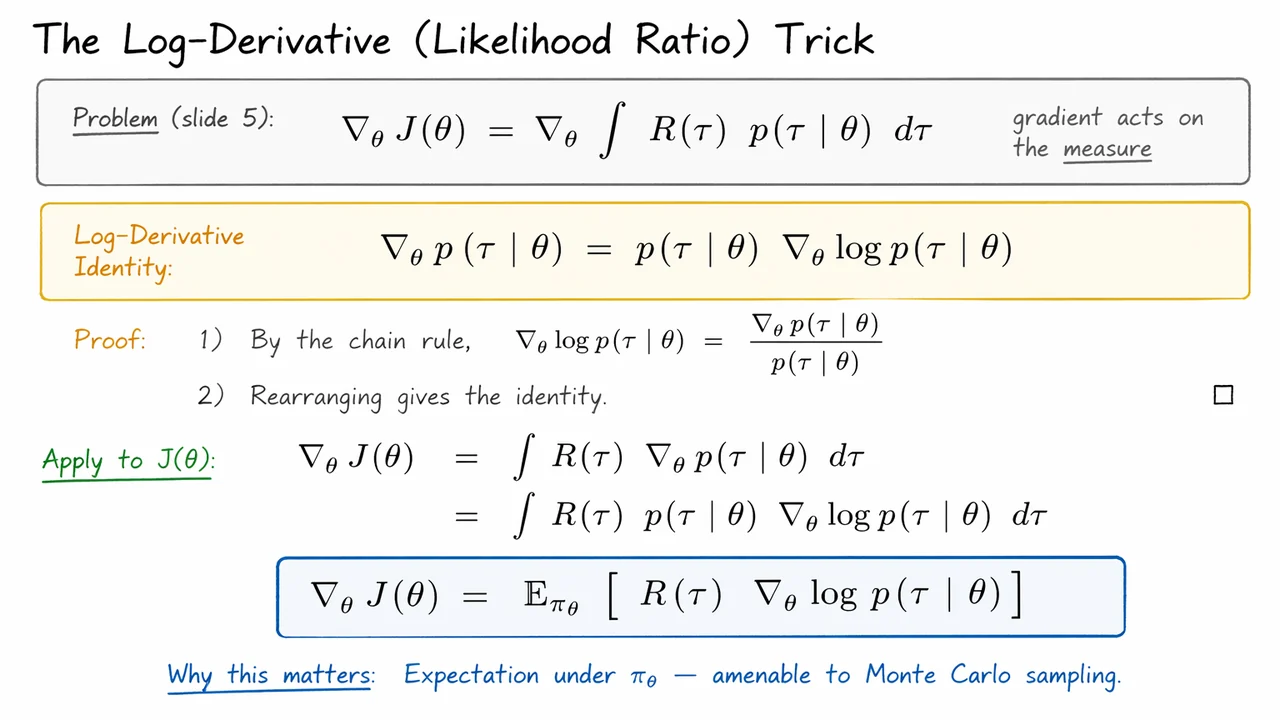
The key move is to rewrite the gradient in a form that isolates the parameter dependence inside a logarithm. For any differentiable density or mass function , the log-derivative identity says
This is just the chain rule in disguise: , so multiplying through by recovers the original gradient. The point of this identity is not aesthetic; it is operational. It turns an awkward derivative of a probability measure into something that looks like an ordinary expectation under the same distribution.
Applying it to the return objective,
we obtain
So the gradient is
This is the essential policy-gradient transformation: the difficult derivative of an expectation becomes an expectation of a score function, i.e. the gradient of the log probability. Once written this way, the gradient can be estimated by Monte Carlo rollouts from the current policy, without differentiating through the environment’s state transitions.
A few subtle points are worth keeping in mind. First, this identity does not make the estimator low-variance by itself. In fact, the raw term is often noisy because the return can fluctuate wildly across trajectories. That is why later we will introduce baselines and advantage functions: they preserve the expectation while reducing variance. Second, the derivation assumes we can exchange gradient and integral under mild regularity conditions; in practice this is usually justified for the smooth parameterizations used in policy networks, but it is still an assumption hiding in the background.
Conceptually, the result matters because it gives us a way to optimize policies in environments where the dynamics are unknown, stochastic, or non-differentiable. The only thing we need to differentiate is the policy’s own log-probability, which is exactly what neural networks can provide. That is why the score-function form is the foundation of REINFORCE, of baseline methods, and eventually of actor-critic algorithms. All of those methods are variations on this same expectation identity.
The visual below compresses that logic into a compact typographic progression. The top reminder isolates the original problem: the gradient is acting on a -dependent measure. The middle identity box captures the whole trick in one line, with the short chain-rule proof underneath to show that nothing mysterious is happening. The bottom derivation then walks from the original integral to the Monte Carlo-friendly expectation, highlighting the exact point where the likelihood ratio form turns a hard calculus problem into a sampling problem.
Read as a whole, the figure is less a derivation than a map of the transformation: from a derivative that seems to require environmental gradients, to a score-function expectation that can be estimated from sampled trajectories. That transition is the conceptual hinge for everything that follows.
Having established the likelihood-ratio identity, the next question is what actually sits inside the trajectory score . This is the point where policy gradients become especially elegant: the trajectory probability factors into pieces generated by the environment and pieces generated by the policy, and only one of those depends on .
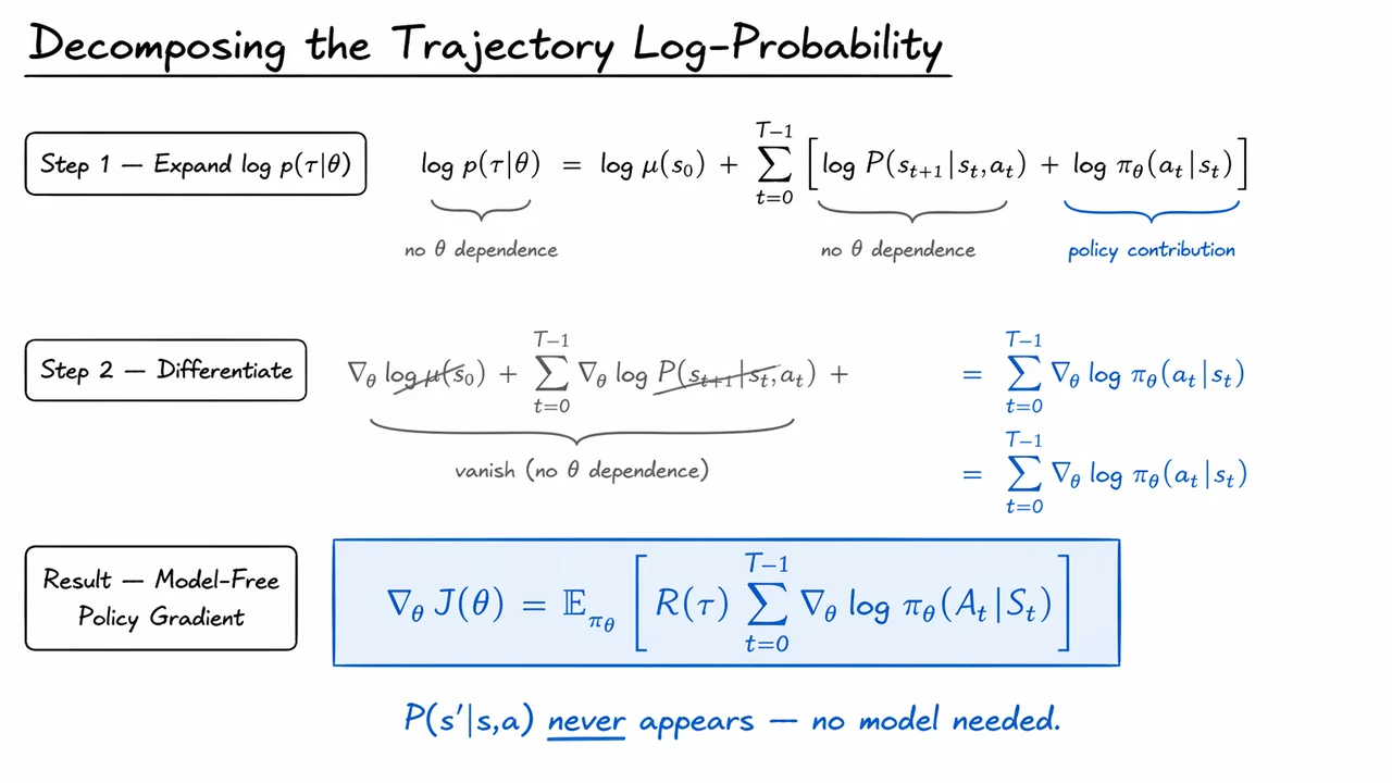
For a finite-horizon trajectory , the joint density under policy is
Taking logs turns the product into a sum:
This decomposition is not just algebraic bookkeeping. It encodes a crucial modeling assumption: the environment evolves according to dynamics that do not change when we adjust the policy parameters . In other words, the policy chooses actions, the environment reacts, but the environment itself is not being differentiated through. That is exactly why the policy gradient method is called model-free: we do not need a differentiable model of the transition kernel to compute the gradient.
Now apply . The initial-state term vanishes immediately, and so do all transition terms , because they are independent of . What remains is just the sum of policy score functions:
This is the heart of the derivation. Every time step contributes a local sensitivity term saying how the log-probability of the sampled action changes if we nudge the policy parameters. The environment still shapes the trajectory, but it contributes only through the realized states and rewards, not through any explicit gradient path.
Substituting this back into the likelihood-ratio form from the previous step yields the familiar REINFORCE estimator:
A useful way to interpret this is as a correlation estimator: trajectories with larger return reinforce the action choices that produced them. The estimator is unbiased, but it is also noisy because the same scalar return multiplies every action score in the trajectory. That variance problem is exactly what motivates baselines, reward-to-go, and actor-critic methods later on.
There is also a subtle but important boundary condition here. The cancellation of relies on the standard policy-gradient setting where the environment dynamics are fixed with respect to . If the policy parameters were to influence the dynamics directly, or if we were learning a differentiable simulator model jointly with the policy, then additional gradient paths could appear. In the classical RL setting, however, the result is clean: the only differentiable object inside the trajectory probability is the policy itself.
So the conceptual message is compact:
The visual below condenses exactly that logic into three steps: expand the log trajectory probability, delete the -independent terms, and arrive at the model-free policy gradient. It is less a new derivation than a proof-of-cancellation, and that cancellation is what makes policy gradient methods practical in unknown environments.
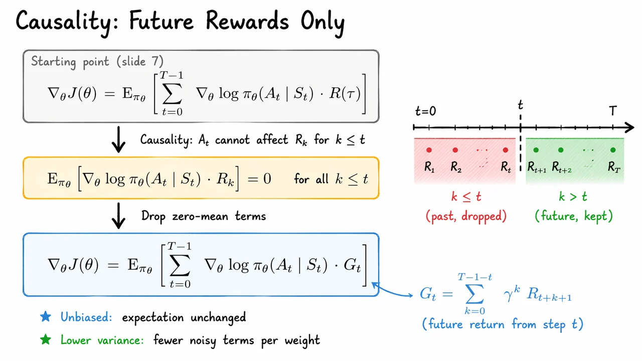
We can now make the policy gradient estimator a little more honest about when information becomes available. The previous form used the full trajectory return with every score term , but that quietly mixes together rewards that happened before action with rewards that happen after it. Intuitively, that is wasteful: if a reward has already occurred, then the action at time could not have caused it.
This is where causality enters. In an MDP, action is selected after observing , and only then does the environment transition forward. So when we ask how the parameters should change to increase expected return, the only rewards that should matter for the decision at time are the ones that lie in its causal future. Past rewards are fixed by the time the action is taken, so they cannot provide a useful learning signal for that action.
Formally, the key observation is a zero-mean identity. For any reward with , the score function term has no positive correlation with that past reward: This is not saying the gradient term is literally zero everywhere; it says that, in expectation, the contribution from rewards that happened before the action cancels out. That cancellation is exactly what lets us simplify the estimator without changing its mean.
So the full-trajectory return can be replaced by the future return from time : With that substitution, the policy gradient becomes This is the causal form of REINFORCE: each action is paired only with the rewards that it could plausibly influence.
The practical benefit is important. We have preserved unbiasedness because we only removed terms whose expectation is zero. But we have also improved the estimator’s variance. Every time we multiply a score term by the full return, we inject noise from rewards that the action could never affect. Removing those irrelevant terms usually makes the gradient signal sharper and learning more stable.
There is a subtle point worth emphasizing: this is not merely a bookkeeping trick. The same return appears in every time step’s gradient estimate, but the relevant portion of that return depends on the time index. The estimator is therefore less like “score times total outcome” and more like “score times the consequences that lie ahead from this decision.” That causal interpretation is what makes the later actor-critic and advantage formulations feel natural rather than ad hoc.
A few takeaways make the logic compact:
The visual summary below organizes exactly this flow: the older full-return expression is shown as the starting point, the causal identity in the middle highlights why the past contributes nothing in expectation, and the final expression keeps only . The small timeline on the side is especially useful because it turns the abstract proof into a picture: the red region marks rewards that are already in the past and therefore dropped, while the green region marks the future rewards that remain attached to the action.
Read that diagram as a compact proof sketch. The arrows are doing the same logical work as the equations: first identify the overcounted past, then invoke causality and zero expectation, and finally arrive at the lower-variance estimator that will power the rest of the policy gradient methods we build next.
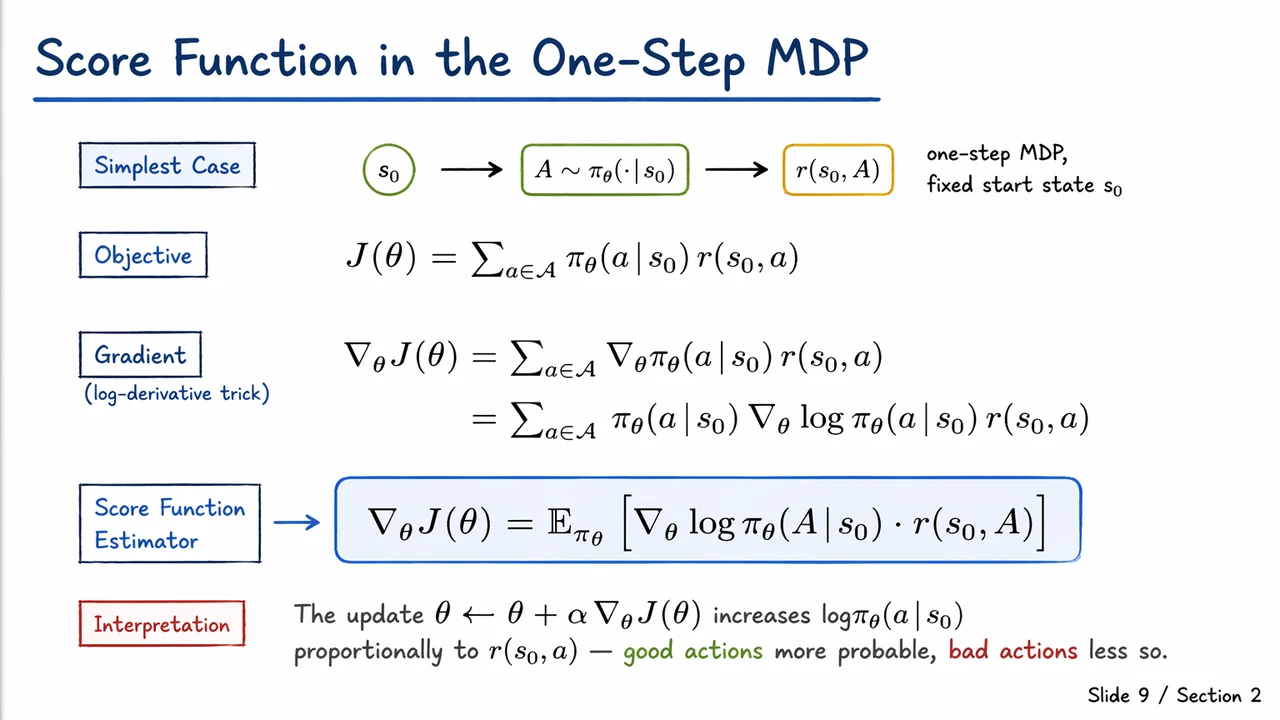
Having established why only future rewards matter, we can now strip the problem down to its cleanest possible form and see the policy gradient mechanism with almost no distractions. The one-step MDP is the smallest setting where the entire idea is already present: there is a fixed start state , we sample a single action , and then immediately receive reward . There is no trajectory credit assignment yet, no return-to-go, and no bootstrapping—just a stochastic choice followed by a scalar payoff.
In this case, the objective is simply the expected reward under the policy: This is the most direct expression of what policy optimization means. We are not trying to predict rewards explicitly; instead, we are adjusting the parameters so that the policy places more mass on actions that empirically lead to higher reward. The dependence on is entirely through the action probabilities.
The key step is to differentiate with respect to . Since does not depend on the policy parameters, it passes through the gradient unchanged: At this point the expression is correct but not yet useful, because it involves directly. The standard trick is to rewrite that derivative in terms of the log-probability: This is just the identity , sometimes called the likelihood ratio trick or log-derivative trick. Its power is that it converts a derivative of a probability into a probability-weighted derivative of a log-probability, which is exactly what we can estimate from samples.
Substituting that identity gives Now the gradient is written as an expectation under the current policy: This is the score function estimator in its most elementary form. The “score” is the gradient of the log policy, and the reward acts as the weight that says how strongly that sampled action should influence the update. High-reward actions push the policy up; low-reward actions push it down.
The intuition is worth stating carefully. Because points in the direction that increases the log-probability of action , multiplying by means:
So the gradient ascent update literally “moves probability mass” toward the better actions. This is the first place where the probabilistic interpretation of policy gradients becomes concrete: we are not editing a value table, we are nudging a distribution.
There is also a subtle but important assumption hiding here: the reward term must be independent of for this derivation to hold in this simple form. In the one-step MDP, that is naturally true because the reward is treated as a function of the chosen action and state, not of the parameters directly. In more general settings, the same idea survives, but the algebra becomes richer because the action influences future states and rewards through the trajectory distribution.
The visual below compresses this chain into a single, readable flow: from the one-step setup, to the expected-reward objective, to the log-derivative rewrite, and finally to the boxed score function estimator. Read it as a compact proof sketch rather than a standalone formula sheet—the point is not just that the identities are true, but that each line prepares the next one by turning an awkward derivative of probabilities into a sample-friendly expectation.
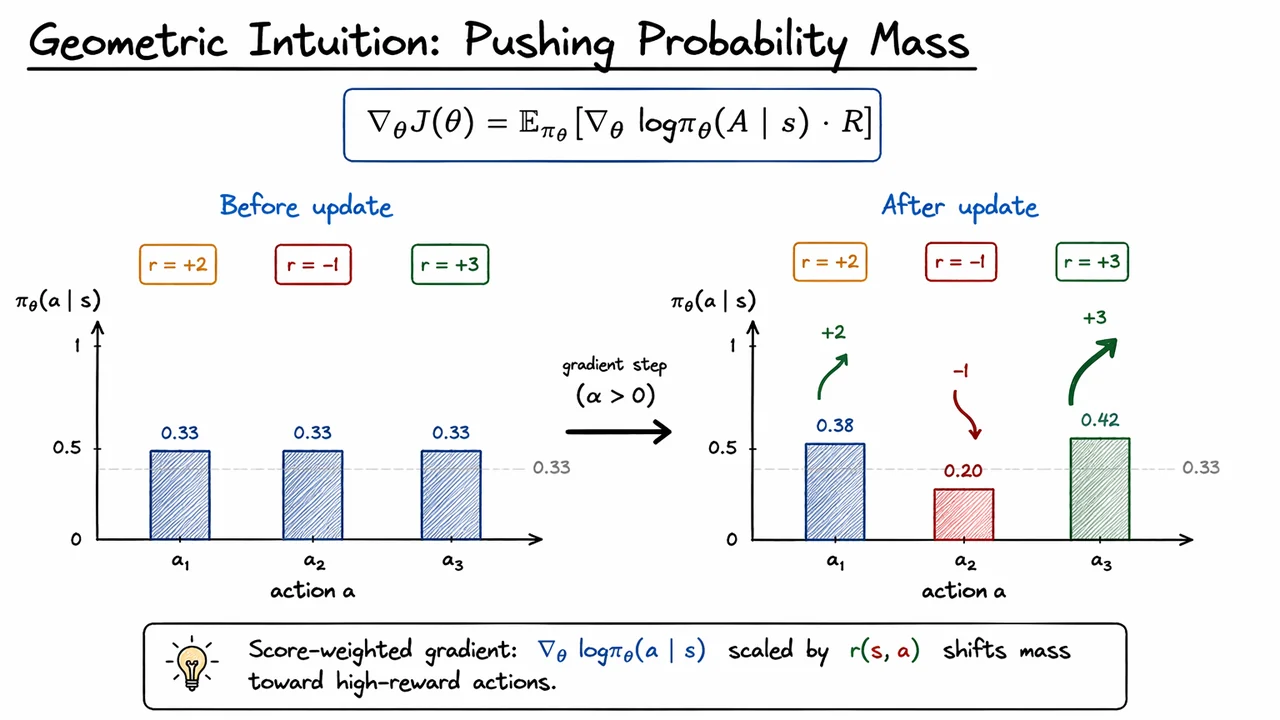
We can now make the score-function update feel geometric rather than merely algebraic. The key question is not just what gradient ascent computes, but how a change in parameters moves the policy itself. For a discrete action space, the policy is a probability distribution over actions, so a gradient step should be understood as redistributing mass across actions, not simply nudging numbers in parameter space.
In the one-step setting, the objective is the expected reward Applying the likelihood ratio trick gives This is already the essential geometric statement: each sampled action contributes a direction in parameter space, and that direction is weighted by how much reward followed that action. If the reward is positive, the update reinforces the probability of that action; if it is negative, the update suppresses it.
A useful way to think about this is to imagine each action carrying its own “vote” in the parameter update. The score function tells us how to increase the probability of locally, and the reward determines how loud that vote is. So the update is a reward-weighted sum of score directions, not an undifferentiated push toward every action equally.
This also explains why the update behaves sensibly in the presence of multiple actions with different payoffs. Suppose we start from a uniform policy over three actions, , with rewards , , and . Then a single gradient step should:
The important subtlety is that the policy update is relative. Because probabilities must still sum to one, increasing mass on high-reward actions necessarily takes mass away from lower-reward ones. This is why policy gradients are often described as pushing probability mass uphill on the reward landscape: the geometry lives on the simplex of categorical distributions, where improvement in one region implies contraction elsewhere.
There is also a deeper connection to reinforcement as a statistical learning principle. The update behaves like a policy-level analogue of Hebbian learning: actions that are “co-activated” with positive reward are strengthened, while actions associated with poor outcomes are weakened. Unlike supervised learning, however, the signal is not a target label; it is a scalar return that only tells us whether the sampled behavior was valuable.
Of course, this clean picture hides the fact that the raw Monte Carlo gradient can be noisy. A single sampled reward may be unrepresentative, and the score function can have large variance even when the direction is unbiased. That limitation is precisely why later variants introduce baselines and critics: they keep the same geometric rule—push mass toward better-than-average actions—while reducing the randomness in how hard each action is pushed.
The visual below compresses this intuition into a simple before-and-after story. Starting from equal probability bars, the update arrow points from the uniform policy to a new distribution where the tallest bar belongs to the highest-reward action, the intermediate reward gets a moderate increase, and the negative-reward action shrinks. The curved arrows are doing more than decorating the diagram: they encode the fact that the gradient acts like a mass transport mechanism, lifting probability where reward is high and draining it where reward is low.
Seen this way, the diagram is not just a summary of a particular example. It is a compact geometric rendering of and of the update Together, they say the same thing: policy gradients do not directly optimize actions; they reshape probability mass so that better actions become more likely.
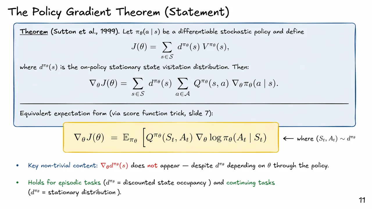
Building on the geometric view from before, we can now state the central identity that makes policy gradients practical: the gradient of performance can be written as an on-policy expectation of a local score term weighted by an action-value signal. This is the point where the optimization problem stops looking like “differentiate through the whole environment” and starts looking like “increase the probability of actions that turn out well.”
Formally, for a differentiable stochastic policy , define the return objective as the expected value under the policy’s own visitation distribution: The notation matters here. The objective is not just a sum of per-state values; it is weighted by , the distribution over states the current policy actually visits. That dependence on is exactly what makes policy gradients seem tricky at first glance. If we differentiate naively, it looks like we should have to backpropagate through both the value function and the state distribution. The theorem says something surprisingly cleaner happens.
The policy gradient theorem states that Equivalently, using the score-function identity , we obtain the compact expectation form This is the form that powers REINFORCE and essentially every modern policy-gradient method. It says: sample from the current policy, evaluate how good the sampled action was in hindsight, and nudge the policy parameters in the direction that makes that action a little more likely.
The subtle, non-trivial part is what does not appear. Although depends on , there is no explicit term in the theorem. That omission is not a shortcut or approximation; it is an exact cancellation that follows from the dynamics of Markov decision processes. Intuitively, the effect of changing the policy on future state visitation is already accounted for indirectly through , because the action-value function captures the downstream consequences of choosing in . In other words, the theorem separates where the policy acts locally from how the environment propagates those choices forward.
This is why the theorem is so useful computationally. If the gradient had to explicitly differentiate through the visitation distribution, we would need a model of the environment dynamics or a full unrolled computation graph of the trajectory distribution. Instead, the theorem gives a model-free policy gradient that only requires sampled trajectories and estimates of or returns. It applies both to episodic tasks, where can be read as a discounted occupancy measure, and to continuing tasks, where it is the stationary state distribution.
A few implications are worth keeping in view:
This theorem is the conceptual bridge between the intuitive “push probability mass toward good actions” picture and the concrete algorithms that follow. REINFORCE will replace with sampled returns ; baselines will subtract variance-reducing terms without changing the expectation; actor-critic methods will learn a low-variance approximation to . All of those variations are easier to understand once this identity is in place, because they are all trying to estimate the same gradient in different ways.
The visual below is best read as a compact summary of that logic. The top portion collects the objective and the theorem statement in symbolic form, while the highlighted expectation form emphasizes the result we actually use in algorithms. The small notes at the bottom are there for two reasons: first, to underline that is absent despite seeming unavoidable; second, to remind us that the theorem covers both episodic and continuing settings. Taken together, the diagram condenses the whole message of the theorem: policy gradients are exact, on-policy, and local in form even though their effect is long-horizon and global in consequence.
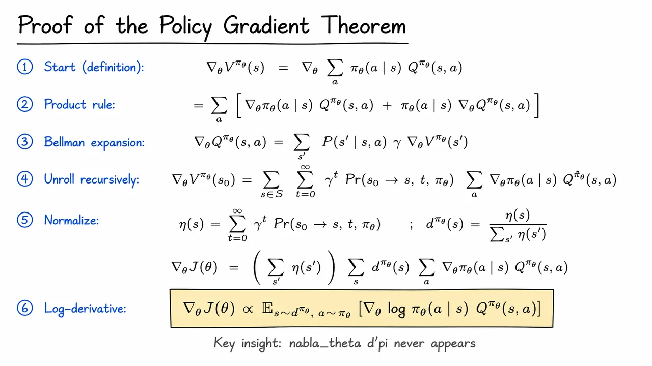
We now have the statement of the policy gradient theorem; the remaining question is why it is true and, just as importantly, why the proof is structured the way it is. The key difficulty is that the objective depends on in two intertwined ways: directly through the policy , and indirectly through the state distribution induced by repeatedly following that policy. A naive differentiation would appear to require tracking how the entire trajectory distribution changes with , which looks hopeless.
The proof avoids that trap by working with the Bellman recursion for the value function. Starting from we apply the product rule: This split is the heart of the argument. The first term already has the shape we want: a policy gradient weighted by action value. The second term is the annoying recursive remainder, but it is also where the Bellman equation earns its keep.
To expand , write the action-value function in one-step form: The transition kernel and reward are environment properties, so they do not depend on . Only the downstream value does. Hence This is the recursive step: the gradient of the value at one state is expressed through the gradient of the value at successor states, discounted by . If you keep substituting this relation forward, the gradient propagates along all possible future trajectories, with each path accumulating a factor of and its corresponding probability under .
That recursive unrolling produces a discounted visitation-weighted sum over states: It is useful to name the discounted occupancy measure This normalization is not just a cosmetic trick: it packages the infinite unrolling into a distribution over states visited under the policy. The important subtlety is that the derivative of this distribution never has to be computed. The proof does not differentiate the state occupancy measure directly; instead, it accumulates the contributions that flow through it, which is why the theorem is so practical.
At this point, the final simplification is the log-derivative trick: Substituting this converts the gradient into the familiar expectation form, The proportionality hides the normalization constant from , but that constant is irrelevant for optimization because it does not change the direction of ascent. What matters is that the gradient can be estimated from sampled trajectories using only terms evaluated along the visited states and actions.
There are two conceptual payoffs here:
That second point is what makes REINFORCE possible, and it also explains why the estimator is so noisy: the theorem gives us a correct unbiased direction, but it does not reduce variance by itself. Baselines, advantage functions, and actor-critic methods will all be refinements of this same identity, designed to replace the raw -signal with lower-variance surrogates while preserving unbiasedness.
The visual below condenses this proof into a compact chain: product rule Bellman recursion discounted unrolling occupancy measure log-derivative form. Read left to right, it emphasizes the one genuinely surprising fact in the proof: the gradient never needs a separate term. That absence is not a loophole; it is the theorem.
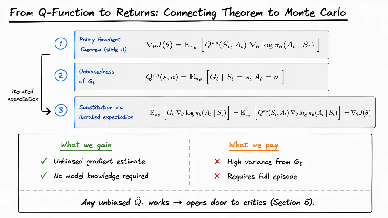
We now have the policy gradient theorem in its cleanest form, but the theorem by itself is still a little too abstract to implement directly. It tells us that the gradient can be written as an expectation involving the action-value function: This is elegant, but it hides a practical problem: is itself unknown. To use the theorem in code, we need some quantity we can actually compute from experience.
The simplest candidate is the Monte Carlo return , the sampled sum of future rewards from time onward. The key identity is that, by definition of the action-value function, This says that is not some unrelated target; it is exactly the conditional expectation of the return after taking action in state and then following the policy. So when we observe one rollout and compute a realized return , we are drawing one sample from the distribution whose mean is .
That observation justifies the Monte Carlo replacement through iterated expectation. If we multiply by the score function and then average over trajectories, the sampled return and the true action-value produce the same expected gradient: The subtle point is that the replacement is not “approximately true” in expectation; it is exactly unbiased as long as is sampled from the correct policy-induced trajectory distribution. This is why Monte Carlo policy gradients are so attractive: they require no model of the environment and no bootstrapping assumptions.
There is, however, an important cost. is a random variable with potentially large spread, especially in long-horizon tasks where each reward is a noisy proxy for eventual success. The estimator is unbiased, but unbiasedness alone does not guarantee usefulness. In practice, a very noisy gradient can make learning unstable, slow, or even appear to fail entirely because updates point in inconsistent directions from episode to episode.
This is the first place where the broader design space of policy gradients becomes visible. The theorem does not demand that we use the exact function ; it only demands an unbiased estimator of it. So any satisfying can be plugged into the same gradient formula without changing the expectation of the update. That freedom is the conceptual bridge to baselines and critics: once you understand that the theorem only cares about the mean of the estimator, you can start trading computation structure for lower variance.
From this viewpoint, Monte Carlo returns are the most direct substitute:
Later, a critic will try to estimate or more smoothly than raw returns, while baselines will subtract a control variate that leaves the mean gradient unchanged. But those are refinements of the same basic logic: replace the unknown with something whose conditional expectation matches it.
The visual below compresses that argument into three steps. The top blocks start with the theorem, then identify as a conditional expectation of , and finally show the substitution justified by iterated expectation. The lower comparison area highlights the real tradeoff: we gain a simple unbiased estimator, but we pay for it with variance. Read as a whole, the diagram is less a new result than a compact proof sketch that explains why the Monte Carlo form is valid and why it is only the beginning of the story.
Up to this point, the policy-gradient story has been about replacing an intractable derivative of environment dynamics with something we can estimate from sampled experience. REINFORCE is the most direct expression of that idea: it takes the Monte Carlo return and uses it as a learning signal for the policy’s score function. In other words, instead of asking, “What action is optimal in this state?” it asks, “Which sampled actions seemed to lead to better returns, and how should I increase their probability?”
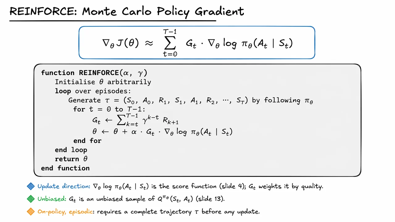
The core estimator is
where the return from time is
This is the most literal Monte Carlo policy gradient: for each visited state-action pair, we compute the total discounted reward that followed it, and then push the parameters in the direction that makes that action more likely. The score function term says how to change the policy locally; the scalar return says whether that sampled decision was good or bad.
A useful way to think about the update is as a form of credit assignment by hindsight. If an action eventually leads to a large return, then the update increases its probability; if it leads to a poor return, the same mechanism decreases its probability. The parameter step is
which is just stochastic gradient ascent on expected return. The elegance here is that the update never needs a model of the environment and never needs an explicit -function approximation. It only needs sampled trajectories and the policy’s own log-probability gradient.
There is, however, an important subtlety: the update is unbiased only because is a Monte Carlo sample of the action-value under the current policy. That means REINFORCE is tied to the data distribution generated by itself. If the episode came from some different behavior policy, then the estimator would no longer be the plain on-policy form; one would need importance sampling corrections. For the basic algorithm, the price of simplicity is that we must collect full trajectories under the current policy before making updates.
That episodic requirement matters practically. Because depends on rewards that occur after time , we cannot update immediately after a single step without either waiting for the episode to finish or introducing additional bootstrapping machinery. This makes REINFORCE conceptually clean but often sample-inefficient: the whole trajectory is used as a delayed training signal, and every action in the episode receives a return-based weight. In long-horizon tasks, those weights can be noisy, especially when many actions have only a weak influence on the final outcome.
The estimator can also be written as a sum of per-time-step gradients, which makes its mechanism easier to remember:
This decomposition is the bridge between the theory and the implementation. The gradient term tells us how to change the policy distribution; the return tells us which sampled decisions deserve reinforcement. Nothing in the update requires a critic, a value baseline, or temporal-difference bootstrapping yet.
The visual below is a compact summary of exactly that logic. The equation at the top captures the policy-gradient estimator in its Monte Carlo form, while the pseudocode box turns the math into an operational recipe: generate a full episode, compute for each time step, and apply the score-function update immediately afterward. The three short callouts reinforce the essential properties that make REINFORCE both attractive and problematic: it is on-policy, unbiased, and episodic.
That combination is what makes REINFORCE the canonical starting point for variance reduction. It is the simplest correct policy-gradient algorithm, and precisely because it is so direct, its weaknesses become easy to see. Those weaknesses are not a flaw in the derivation; they are the inevitable consequence of using raw Monte Carlo returns as the learning signal.
After establishing that REINFORCE gives us an unbiased policy gradient estimate, the next question is the one that matters in practice: why does it still feel so unstable? The answer is variance. Unbiasedness only says that, in expectation, the estimator points in the right direction; it says nothing about how wildly individual samples may deviate from that direction. In policy gradient methods, those deviations can be so large that learning becomes painfully slow, even though the underlying objective is theoretically correct.
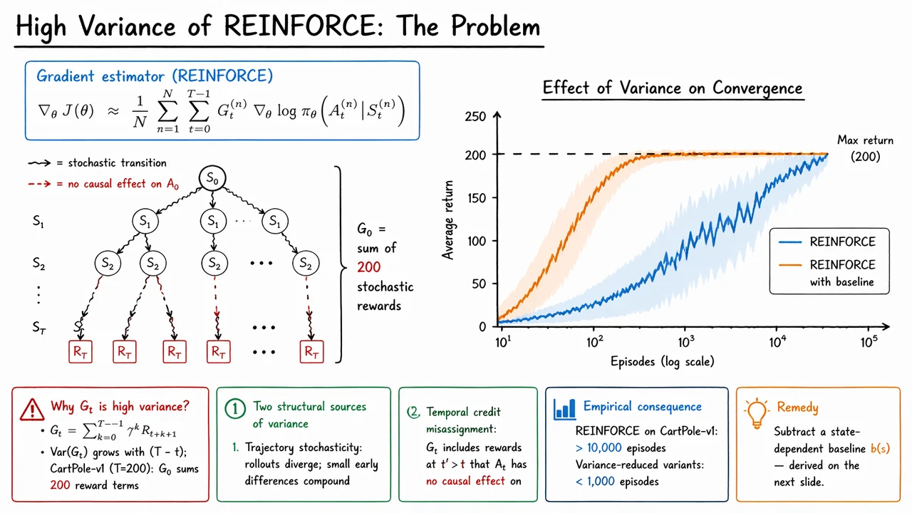
The core estimator is
This looks deceptively simple: each action gets weighted by the return observed after it, and the average over many rollouts approximates the true gradient. But the quantity doing the heavy lifting here is , the Monte Carlo return from time ,
That sum is where the trouble begins. It aggregates a long chain of stochastic rewards, and the longer the horizon, the more random terms accumulate. A useful mental model is that the variance of grows roughly with the remaining episode length:
So early actions are evaluated using the noisiest return estimates, because they depend on the entire future of the trajectory. In environments like CartPole-v1, where an episode can last 200 steps, the first few updates are effectively tied to sums of hundreds of random reward contributions.
There are really two different sources of noise here. First, trajectory stochasticity: even if we start from the same policy, small differences in sampled actions cause trajectories to diverge, and those divergences compound over time. Second, temporal credit misassignment: the return includes rewards that happened after action , even when that action had little or no causal influence on them. The gradient update therefore treats distant rewards as evidence about nearby decisions, which is statistically legal but often semantically misleading.
This distinction is important. The estimator remains unbiased because, in expectation, the log-derivative trick correctly attributes score to the policy's chosen actions. But high variance means a single episode can push the parameters in a very different direction from the next episode, even when both are sampled from the same policy. In effect, the learning signal is correct on average but too noisy to be useful without some form of variance reduction.
That is why REINFORCE often converges so slowly in practice. On CartPole-v1, vanilla Monte Carlo policy gradients may require more than 10,000 episodes to become reliable, while methods that reduce variance can reach the same performance in under 1,000. The difference is not that the objective changes; it is that the estimator becomes less distracted by irrelevant fluctuations. The most direct fix is to subtract a baseline , ideally one that depends on the state but not on the sampled action. Intuitively, this recenters the learning signal so that only relative advantage matters.
A few takeaways are worth keeping in mind:
The visual below compresses these ideas into two complementary pictures. On the left, the trajectory tree makes the credit problem concrete: early actions must “inherit” a noisy return built from many future rewards, and the red distant nodes emphasize how much of that signal is only weakly connected to the action being updated. On the right, the learning curves turn the statistics into an empirical story: the same algorithm that is mathematically sound can still crawl, while a variance-reduced version climbs much faster toward the optimal return. Together, they motivate the next step: subtracting a baseline to preserve correctness while taming the noise.
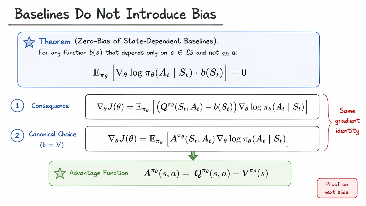
We now have the key variance-reduction idea in hand: subtract something that helps numerically, but contributes nothing in expectation. In policy gradients, that “something” is a baseline that depends only on the state. The subtle point is that this is not an ad hoc trick—it is an exact identity that follows from the way the policy gradient is constructed.
Start from the REINFORCE form of the gradient, where the policy is weighted by a return-like signal. If we replace with , the gradient remains unchanged as long as does not depend on the sampled action. The reason is that the expected contribution of the baseline vanishes: This identity is the heart of the theorem. It says the baseline can reduce variance without shifting the mean of the estimator, so we are not trading bias for stability. We are only changing the spread of the Monte Carlo signal.
Why does the expectation collapse to zero? Condition on the state . Then is just a constant with respect to the action draw , so assuming a discrete action space; the continuous-action version uses the same normalization argument with an integral. This is the quiet but important structural fact behind baseline methods: the score function always integrates to zero under the policy that generated the sample.
Once that identity is in place, the policy gradient theorem immediately admits the centered form This is the same gradient, just rewritten with a better-conditioned learning signal. Intuitively, the policy no longer asks, “Was this return large in absolute terms?” It asks, “Was this action better or worse than what I would typically expect from this state?”
That interpretation becomes especially clean with the canonical choice . Then the centered return becomes the advantage function and the gradient takes the compact form This is conceptually important because it separates two roles that REINFORCE had been mixing together:
The variance reduction matters because the raw return can be dominated by environment noise, horizon length, and reward scale, all of which obscure the learning signal. A baseline removes the predictable state-dependent component, often making updates much smaller in variance and therefore much more stable. But the theorem also clarifies a common failure mode: if the baseline depends on the action, then the zero-expectation argument breaks, and bias can creep in unless the correction is handled carefully.
So the real lesson is not merely that baselines are “allowed,” but that they are mathematically free so long as they remain state-only. That freedom is what lets us build actor-critic methods: the critic learns a baseline, usually , while the actor receives the advantage-weighted policy gradient. The result is a more efficient estimator that preserves the exact objective.
The visual below compresses this argument into a compact theorem-style layout. The upper block states the zero-bias identity itself, while the lower equations show the two natural rewritings: first with an arbitrary baseline , and then with the canonical choice . Read together, they make the logic almost mechanical: subtract a state-only function, keep the same expected gradient, and interpret the remainder as advantage.
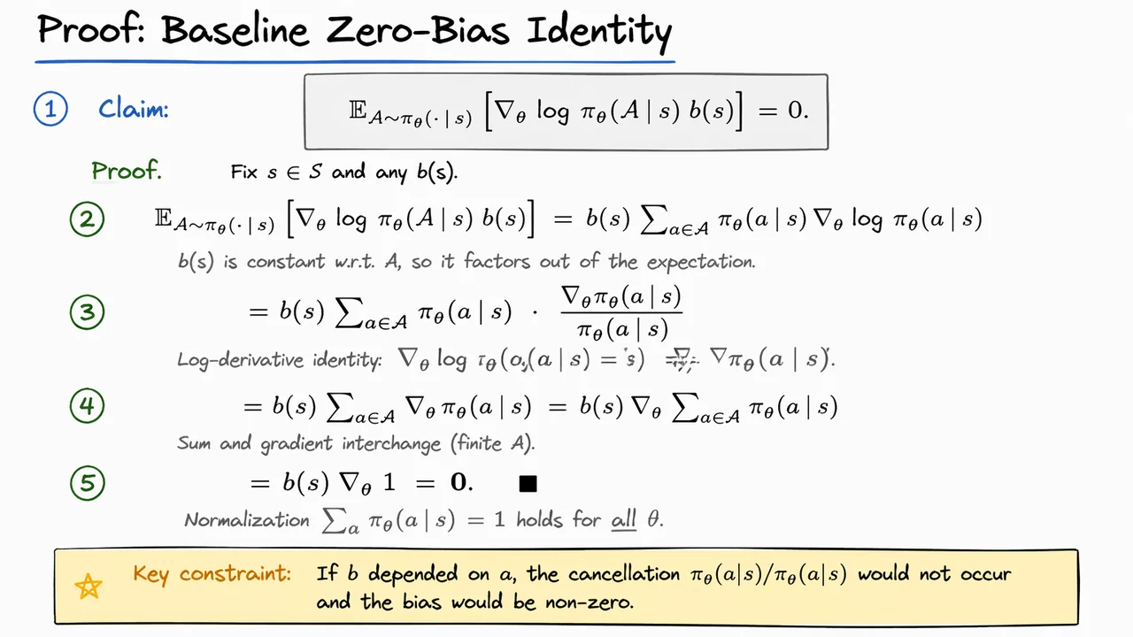
We now have the key algebraic ingredient that makes baselines useful in policy gradients: they can reduce variance without changing the expected update. The essential point is that a baseline must depend only on the state , not on the sampled action . That restriction is what turns the baseline term into something that averages to zero under the policy.
To see why, fix a state and consider the random action . The baseline contribution to the policy-gradient estimator is At first glance this looks nontrivial, because is a random vector that depends on the sampled action. But is fixed once the state is fixed, so it can be pulled outside the expectation. The remaining expectation is just the expected score function under the policy.
Now the important identity enters: for discrete actions, Substituting this into the sum over actions causes the policy probability to cancel, leaving This is where normalization does the real work. Since for every , differentiating both sides gives So the whole baseline term vanishes in expectation.
That cancellation is the reason baselines are so attractive in REINFORCE-style methods: they can change the spread of the estimator without changing its mean. Put differently, the baseline acts as a control variate whose expectation is exactly zero under the current policy. The policy-gradient estimate stays unbiased, but its variance can drop dramatically if tracks the typical return from that state.
There is also a subtle failure mode worth keeping in mind. The argument breaks the moment the baseline depends on the action. If were , then it would no longer factor out of the expectation, and the cancellation would not go through. In that case the “baseline” would generally introduce bias rather than remove variance. This is why, in policy-gradient practice, baselines are usually implemented as state-value functions or approximations to them.
This proof also explains why advantage functions are so natural. If we write then the subtraction of is exactly the kind of zero-mean baseline we just proved harmless. The update can then use the advantage instead of the raw return, which tends to center the learning signal around what is better or worse than expected rather than what is merely large in absolute terms.
The visual below compresses that algebra into a compact chain of equalities: factor out the state-only baseline, rewrite the score function with the log-derivative identity, cancel the policy in numerator and denominator, and finally invoke normalization to reach zero. The boxed remark at the bottom highlights the only real constraint in the argument: action-independence. Once that is clear, the result becomes a reusable lemma for the next step, where we turn this identity into the practical REINFORCE with baseline estimator.
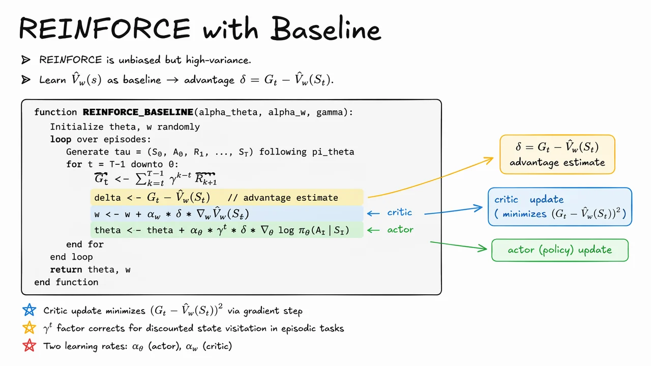
After the zero-bias baseline identity, the natural next step is to ask: if any state-dependent baseline is allowed, what baseline should we actually learn? The answer is to estimate the state value , because it is the most obvious quantity whose scale matches the return and therefore can remove a large fraction of the variance in the policy-gradient signal. In practice we do not know , so we fit a parametric approximation and use it as a learned baseline.
This gives the familiar advantage-style update where is the Monte Carlo return from time , The quantity is not just a heuristic error term: it is the return centered by the critic’s prediction. If is accurate, then is small for actions whose outcomes were ordinary and large in magnitude for unexpectedly good or bad outcomes. That makes the policy update much less noisy than plain REINFORCE, while preserving the same expected gradient as long as the baseline depends only on the state.
The algorithm therefore has two coupled learning problems. The critic learns to predict returns by minimizing a squared-error objective, while the actor uses the resulting advantage estimate to update the policy. The critic step is which is just stochastic gradient ascent on or equivalently gradient descent on the prediction error. The actor step is Here the same drives the policy update, but now it is weighted by the score function , which tells us how to change the probability of the sampled action. Positive advantage increases the action’s log-probability; negative advantage decreases it.
A subtle but important detail is the factor . In episodic problems, the policy gradient theorem can be written as an expectation over discounted state visitation, and that discounting appears in the per-step contribution when we expand the gradient into an episode-wise sum. If you omit it in this formulation, you implicitly change the weighting of earlier versus later decisions. It is one of those bookkeeping factors that is easy to overlook but essential for matching the theoretical objective.
The resulting method is often described as REINFORCE with baseline, but it is more revealing to think of it as the first actor-critic algorithm in miniature:
This is precisely why the method reduces variance without introducing bias: subtracting changes the center of the learning signal, not its expectation, provided the baseline is state-dependent and not action-dependent. In other words, the critic is allowed to reshape the noise, but not to change which direction is correct in expectation.
There is also a practical reason to keep the critic and actor learning rates separate. The critic should usually track the moving target quickly enough to stay informative, but not so aggressively that it becomes unstable. The actor, meanwhile, should move more cautiously because it is optimizing the actual policy objective. When the critic is undertrained, remains noisy; when it is overconfident but inaccurate, the actor can be pushed in poor directions. So the two-step update is simple, but the interaction is delicate.
The visual below compresses all of that into a compact algorithmic picture: the top reminds you that the method is still REINFORCE at heart, the center shows how the return is turned into an advantage via the learned value baseline, and the highlighted lines separate the critic update from the actor update. That split is the key conceptual move. Once you can read the pseudo-code as “estimate value, form advantage, update critic, update policy,” the whole method becomes easy to place inside the broader bias-variance story.
It also prepares the ground for what comes next. REINFORCE with baseline still uses full Monte Carlo returns, so it keeps the low-bias, high-variance character of sampling complete episodes. The baseline makes the signal cleaner, but it does not yet bootstrap from incomplete future predictions. That is exactly the transition point to the next idea: how to trade Monte Carlo targets for bootstrapped ones in order to push variance down further, at the cost of introducing controlled bias.
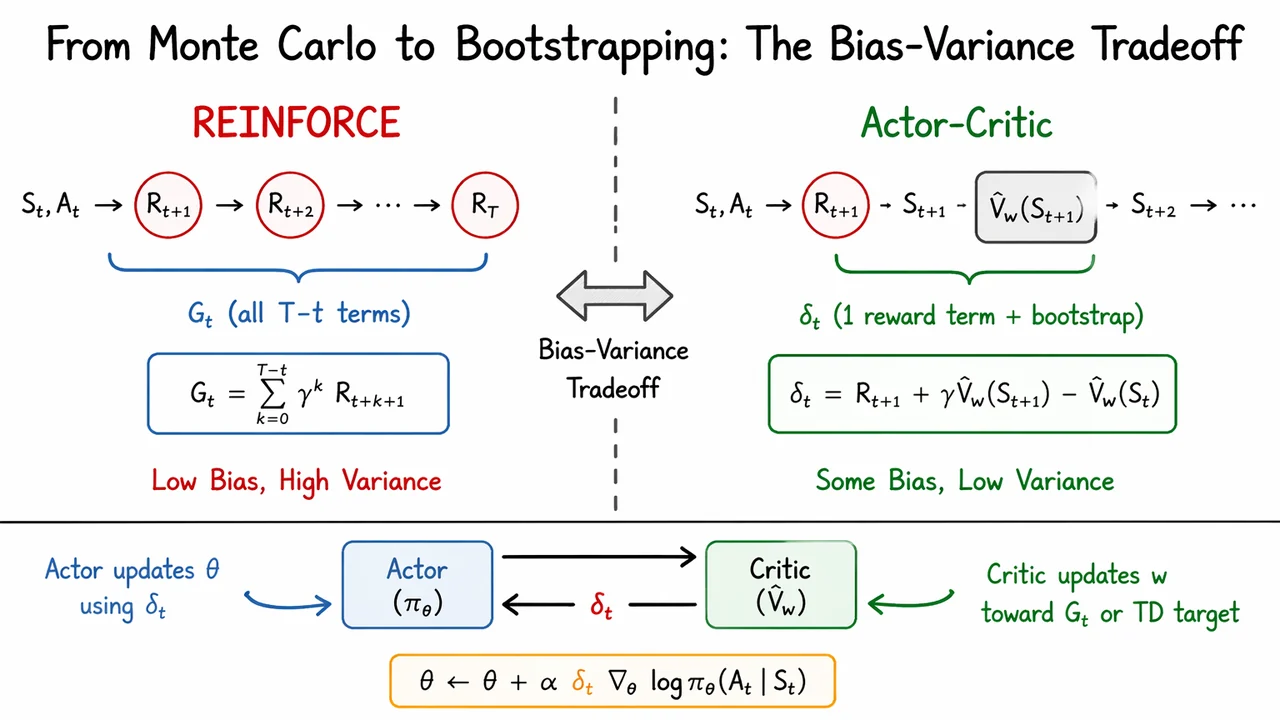
After introducing a baseline, the natural next question is: why stop at subtracting variance from a Monte Carlo return if we can estimate the return itself more aggressively? The answer is the core idea behind actor-critic methods. Instead of waiting until the end of the trajectory to compute the full return , we let a learned value function supply a bootstrapped estimate of the future. That move replaces “sum everything you will ever see” with “use what you have now, plus a guess about what comes next.”
For REINFORCE, the return is
which is conceptually clean: if you sample complete trajectories from the current policy, is an unbiased target for . But that unbiasedness comes at a price. Every additional future reward term injects randomness, so as the horizon grows, the target becomes increasingly noisy. In long episodes, the policy gradient is then driven by a signal that is correct on average but volatile from sample to sample.
Bootstrapping changes the estimator from “roll out all the way to the end” to “stop after one step and consult a critic.” A common one-step target is
This is a much smaller random object: only the immediate reward is sampled directly, while the rest of the future is summarized by . The variance drops sharply because we no longer accumulate a long chain of stochastic rewards. The tradeoff is that is only an approximation, so is generally biased relative to the true action-value function. In other words, we are no longer guaranteed to point exactly toward the true gradient direction at every step.
The same idea can be expressed even more locally through the TD error
This quantity is best understood as an advantage-like correction: if the observed outcome is better than the critic predicted, and the actor increases the probability of the chosen action; if worse, the probability is decreased. If the critic were perfect, meaning , then would be an unbiased sample of the advantage . In practice, the critic is imperfect, so the update is biased—but often only mildly so, and that small bias is a worthwhile payment for a much cleaner learning signal.
This is why the actor update becomes
Notice the structural beauty here: the policy gradient still has the same likelihood-ratio form, but the return estimate has been replaced by a critic-generated teaching signal. The actor does not need a full Monte Carlo return anymore; it only needs a scalar that says whether the recent action was better or worse than expected. Meanwhile, the critic is trained to reduce its own prediction error, so the two components co-evolve.
The essential lesson is the bias-variance tradeoff:
The visual below is useful precisely because it compresses that tradeoff into a single comparison. The left side emphasizes how REINFORCE spreads credit across an entire reward sequence, which is statistically faithful but noisy. The right side shows the actor-critic compromise: one immediate reward, one bootstrapped estimate, and a TD error that serves as the actor’s training signal. Read together, the two panels make the central point tangible—actor-critic methods are not abandoning policy gradients, but approximating their targets in a way that dramatically lowers variance while accepting controlled bias.
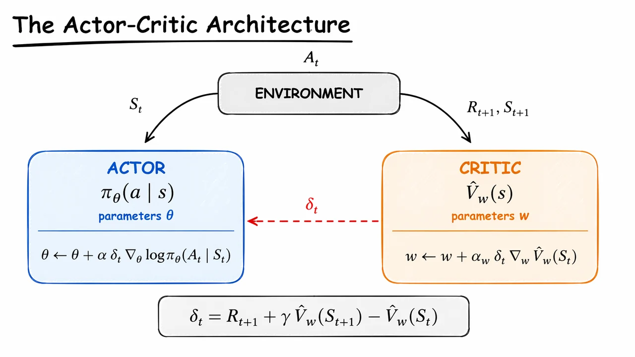
Building on the bias–variance tradeoff, the actor–critic architecture makes a very practical compromise: instead of waiting for a full return to score an action, we let a learned critic provide a fast, local evaluation signal to a learned actor that controls behavior. This keeps the policy-gradient machinery intact, but replaces the noisy Monte Carlo target with something that can be formed at every step.
The key idea is that we now maintain two separate parameter vectors with different jobs. The actor is the policy , and its only responsibility is to choose actions that increase the objective . The critic is a value approximator , whose job is to estimate how good the current state is under the current policy. Because these components learn different quantities, they do not share parameters: is updated to improve control, while is updated to improve prediction.
What makes this architecture interesting is that the critic does not merely predict state values for their own sake; it also produces an advantage-like signal for the actor. The one-step temporal-difference error is If , the outcome was better than the critic expected, so the taken action should be reinforced. If , the outcome was worse than expected, so the actor should reduce the probability of repeating that action in that state. In that sense, plays the same conceptual role as an advantage estimate.
The critic itself is usually trained by a semi-gradient TD(0) update: This is a prediction problem, not a control problem. The critic tries to make its current estimate agree with a bootstrapped target , which means it can learn from a single transition rather than waiting for episode termination. That is the source of the lower variance: we are no longer averaging over long return trajectories.
The actor then uses the critic’s signal as a multiplicative weight on the policy-gradient direction: This has the same structural form as REINFORCE with a baseline, except that the baseline has been replaced by a bootstrapped estimator. The benefit is immediate feedback and much smaller variance; the cost is that is now biased because it depends on , not the true value function. In practice, that tradeoff is often worth it, especially when episodes are long or returns are extremely noisy.
A useful way to think about the whole system is:
This division of labor is what gives actor–critic methods their flexibility. They unify Monte Carlo-style policy improvement with bootstrapped value learning, and they scale well when full returns are expensive or variance would otherwise dominate the gradient estimate. The main caveat is that the actor is only as good as the critic’s signal; if the critic is inaccurate or unstable, the policy update can be misled, even though it is lower variance.
The visual below compresses exactly that relationship into a compact update loop. The two large boxes separate the roles of policy and value estimation, while the arrows make the information flow explicit: state goes to the actor, action goes back to the environment, reward and next state feed the critic, and the critic sends back as the learning signal. The equation at the bottom then ties the whole diagram together by showing that the scalar driving both updates is just a one-step TD error.
That compact summary is important because it reveals the core identity of actor–critic methods: they are not two unrelated algorithms glued together, but a single learning system in which a learned evaluator shapes the policy update step by step.
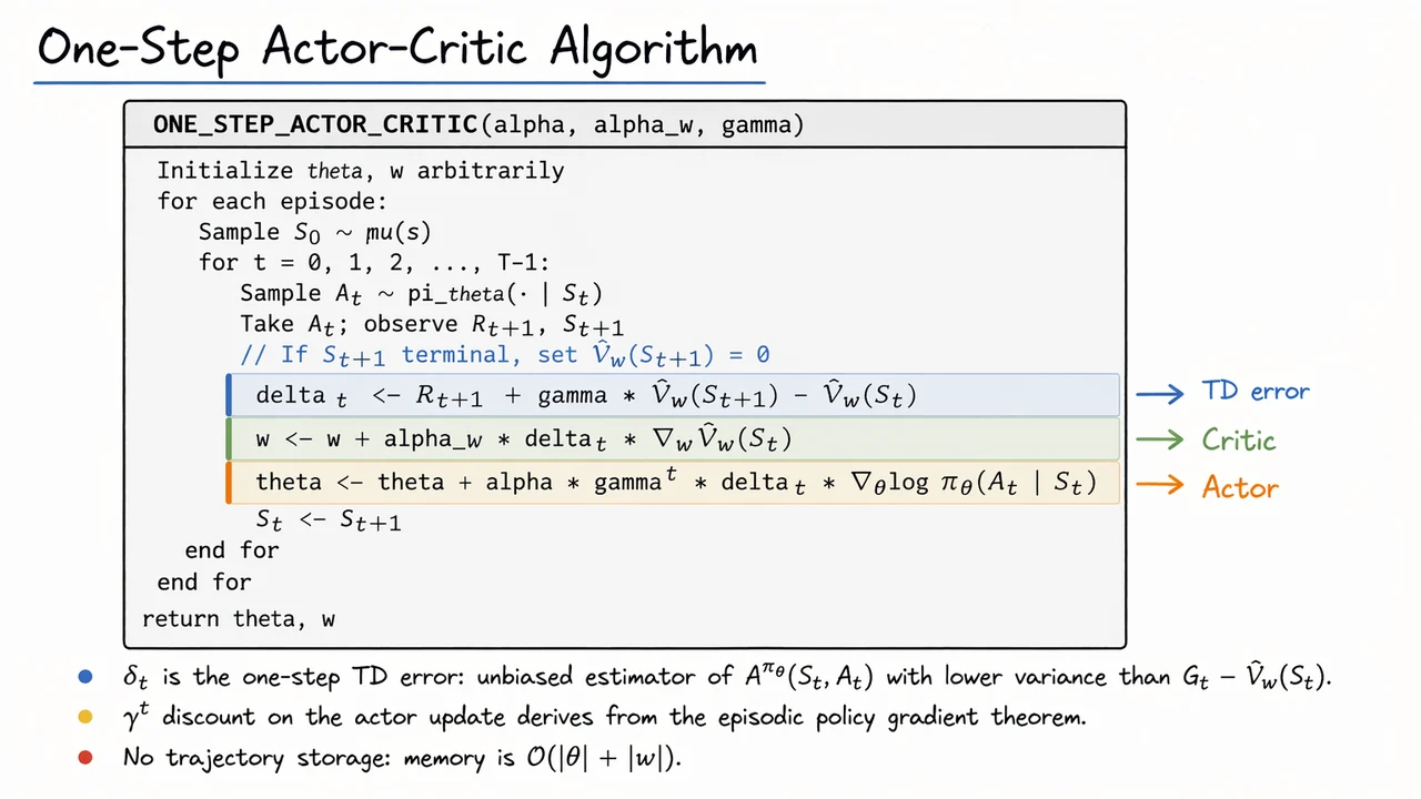
We can now make the leap from Monte Carlo actor-critic to a truly online algorithm. The key observation is simple but powerful: the actor does not actually need to wait until the end of the episode to get a learning signal. Instead of using the full return , we can bootstrap from the critic’s current value estimate and use a one-step target. This trades exactness for immediacy, and in policy-gradient methods that is often the right exchange.
Formally, define the temporal-difference error This quantity compares what the critic expected at state with what actually happened after one transition. If , the transition turned out better than expected; if , it was worse. That is why is so useful: it behaves like a noisy estimate of the advantage , but is available immediately after observing the next reward and state.
The critic update is then just standard TD learning with function approximation: Intuitively, the critic moves its value estimate in the direction that would have reduced the one-step prediction error. If the critic is well behaved, this update makes track the current policy’s value function, which in turn makes the actor’s updates less noisy than plain REINFORCE. Of course, this comes with the usual caveats: with nonlinear function approximation, bootstrapping, and off-policy data, stability can become delicate. In the on-policy setting we are considering here, though, the update remains the cleanest online baseline one can reasonably hope for.
The actor update uses the same as a surrogate for the advantage: The factor is not cosmetic; it comes directly from the episodic policy gradient theorem. Earlier, when we derived the gradient of the discounted objective, each time step’s contribution was weighted by . The one-step actor-critic preserves that structure while replacing the high-variance Monte Carlo return with a local, bootstrapped signal. This is what makes the algorithm both online and still faithful to the underlying policy-gradient objective.
A useful way to see the logic is to compare the estimator forms:
That last point is subtle. The critic is not merely a learned baseline here; it is also the mechanism that defines the temporal-difference target. So the actor and critic are coupled more tightly than in baseline-only REINFORCE. If the critic lags too far behind, the actor may be chasing a moving target; if the critic is accurate enough, the TD error becomes a much cleaner learning signal than raw returns.
Another advantage is practical rather than statistical: there is no trajectory storage. The algorithm updates immediately after each transition, so memory scales as rather than with episode length. That matters in long-horizon tasks, continuing tasks, and any setting where waiting until the end of an episode would be inconvenient or impossible.
The visual below compresses exactly these ideas into a compact algorithmic form. The highlighted line emphasizes that the TD error is the hinge between critic and actor: it first updates the value function, and then it becomes the weighted signal that pushes the policy parameters. The blue, green, and orange accents are not just decorative; they correspond to the error signal, the critic update, and the actor update, respectively, making it easy to see how one observed transition drives both learning systems.
Just as importantly, the boxed pseudocode also makes the computational story explicit. You can read it as an online loop: sample an action, observe the next reward and state, compute , update the critic, update the actor, and move on. That sequence is the essence of one-step actor-critic: a small modification to REINFORCE-with-baseline, but one that changes the algorithm from an episodic estimator into a fully streaming policy-gradient method.
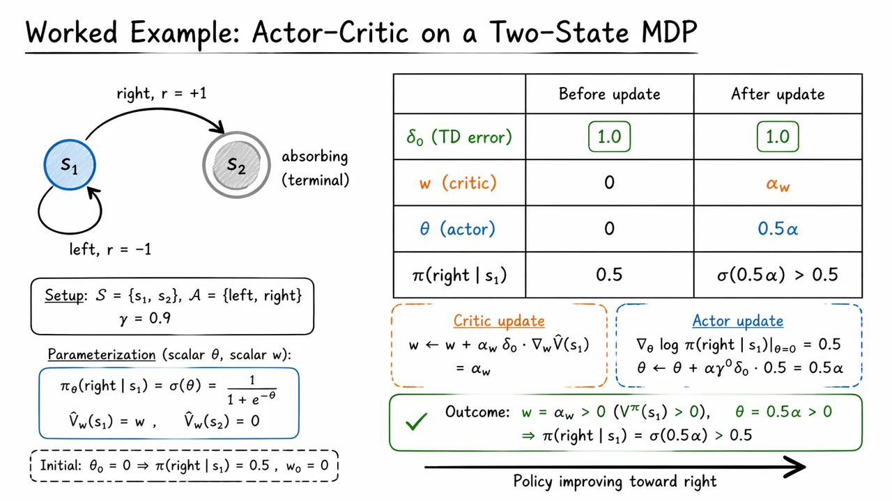
Having established the one-step actor-critic update in abstract, it helps to anchor the formulas in a toy environment where every quantity can be computed by hand. The point of this example is not complexity; it is clarity. With only two states and two actions, we can watch the critic estimate a value, the actor shift the policy, and the temporal-difference error couple the two updates in real time.
Consider the MDP with , , and discount . State is absorbing, while state is the only decision point. The reward structure is deliberately asymmetric: So the optimal behavior is obvious in hindsight: always choose right. But the algorithm does not know that in advance. It must infer it from sampled experience, which is exactly why this tiny problem is useful.
We use the simplest possible parameterization: a scalar policy parameter and a scalar value parameter . The actor is a logistic policy, and the critic predicts Starting at means the policy is initially indifferent: . Starting at means the critic initially believes has zero value. That symmetry is important, because it makes the first update easy to interpret: any movement is due to the observed transition, not to a prior preference baked into the parameters.
Now suppose the agent samples , receives , and transitions to . Because is terminal, , so the TD error is This single number drives both updates. The critic performs a semi-gradient step toward the observed return: So the value estimate becomes positive immediately, which is exactly what we want: after seeing a rewarding transition from , the critic should raise its estimate of how good is.
The actor receives the same TD error as a learning signal, but now it is modulated by the score function term: Therefore the policy update is Because increases, the probability of choosing right also increases: This is the essential actor-critic mechanism in miniature: the critic says, “that outcome was better than expected,” and the actor responds by making the responsible action more likely.
A few subtleties are worth noticing. First, the actor does not update directly from reward alone; it updates from advantage-like information encoded in . If the reward had been worse than expected, would be negative and the policy would move in the opposite direction. Second, the critic and actor are coupled but not identical: the critic learns a baseline value function, while the actor uses the critic’s residual error as a direction of improvement. This is precisely how actor-critic methods reduce the variance of pure Monte Carlo policy gradients without introducing bias from an unrelated baseline.
The visual below condenses that entire chain of reasoning into one glance. The left side isolates the MDP structure: a single decision state, two actions, and the absorbing terminal state that makes the return easy to compute. The right side then aligns the pre- and post-update values for , , , and , so you can see the co-evolution of critic and actor rather than treating them as separate algorithms.
Read it as a compact proof by example: a positive TD error raises the critic’s estimate of and simultaneously nudges the policy toward the action that caused the improvement. That concrete feedback loop is the bridge from this one-step update to the more general variance-reduction ideas that come next, including multi-step returns and generalized advantage estimation.
After seeing how a one-step critic turns raw rewards into the temporal-difference error , the natural question is how far we should propagate information before handing it to the policy update. A single TD step is attractive because it is cheap and local, but it can be too local: it trusts the critic’s bootstrapped estimate heavily, so any systematic value-function error leaks directly into the advantage estimate. At the other extreme, the Monte Carlo advantage waits until the end of the trajectory, which removes bootstrapping bias but makes the update noisy, especially in long-horizon tasks.
This is exactly the bias–variance tradeoff in actor-critic form. If we write the -step return as then increasing moves us closer to a Monte Carlo target. That generally reduces bias because we rely less on the critic’s one-step extrapolation, but it also raises variance because more of the target depends on sampled rewards. In practice, no single is uniformly best across training phases or tasks, so a fixed horizon can be a brittle design choice.
Generalized Advantage Estimation (GAE) replaces the hard choice of one with a smooth mixture over all future TD residuals: This formula is elegant because it says: don’t commit to a single backup length; average them with exponentially decaying weights. Early TD errors get the most influence, later ones still matter, and the parameter controls how quickly that influence fades. In other words, is a soft horizon parameter.
The two boundary cases make the interpretation precise:
So GAE is not a new target in the sense of inventing a different objective; it is a particular way of estimating advantage that interpolates between two familiar extremes. The main practical benefit is that policy optimization often cares more about getting the direction of improvement right than about perfectly unbiased advantages. A slightly biased but much lower-variance estimate can produce faster and more stable learning than an unbiased estimate that thrashes the policy gradient with noise.
There is also a useful conceptual link to -step returns. GAE can be viewed as combining the advantages implied by all -step targets, with exponentially decaying weights determined by . That means it inherits the multi-step propagation benefits of longer backups while retaining the stability of short backups. The common default is popular precisely because it tends to keep enough trace of future rewards without letting variance explode; paired with , it usually yields a long but controlled effective horizon.
A subtle but important assumption here is that the baseline is state-dependent but not action-dependent. That preserves the policy gradient’s correctness while reducing variance; if we were to use an action-dependent correction carelessly, we could distort the update direction. GAE fits cleanly into the actor-critic framework because it is still just an advantage estimator—a replacement for , not a change to the underlying policy-gradient theorem.
The visual summary below helps because the whole story is really about a continuum. The upper part compresses the two mathematical anchors: the -step return on one side and the GAE residual sum on the other. The lower spectrum then makes the tradeoff tangible: as moves from to , we slide from one-step TD toward Monte Carlo, trading variance for bias in a controlled way. The marked default around is a reminder that practical algorithms usually live in the middle, not at either endpoint.
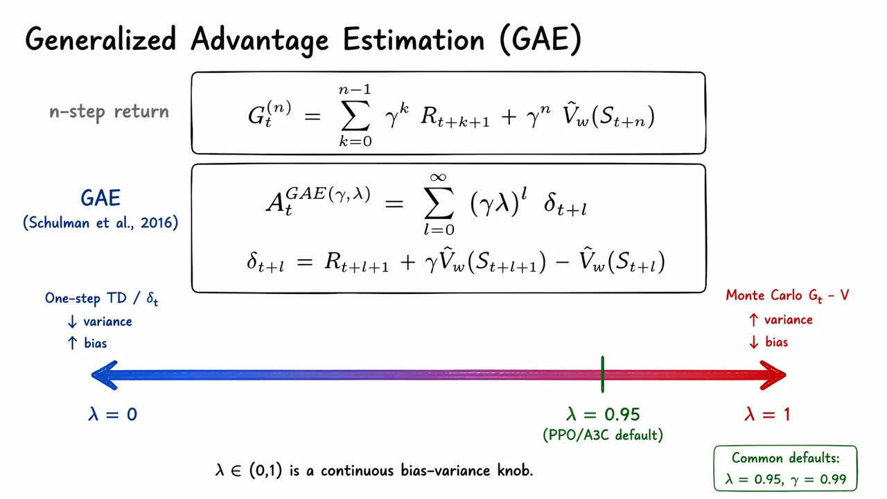
After GAE gives us a cleaner estimate of advantage, the next question is almost unavoidable: why keep throwing away experience? In vanilla REINFORCE and many actor-critic implementations, once a trajectory has been used to update the policy, it is typically treated as stale. That makes the mathematics simple—our samples are drawn from the very policy whose gradient we want—but it is also painfully wasteful. A policy rollout may contain rich information about state visitation, action preferences, and reward structure, yet the algorithm effectively consumes it once and discards it.
This inefficiency is especially glaring when compared with value-based methods such as DQN, which are built around replay. There, a single transition can be revisited many times because the target is not tied so tightly to the current policy distribution. For policy gradients, the obstacle is subtler: the objective is an expectation under the current policy , so if the data were generated by an older policy , then naïvely treating those samples as current would introduce bias. In other words, the data are not wrong—they are just drawn from the wrong distribution.
The standard fix is importance sampling. The idea is to correct for the mismatch between the behavior policy that generated the data and the target policy we now want to optimize. For a single timestep, the correction factor is
If the new policy assigns higher probability to the sampled action than the old policy did, then and that sample is upweighted; if the new policy likes it less, the sample is downweighted. This is a principled way to reuse old trajectories while still estimating the gradient of the current objective.
Putting this into the policy gradient gives the familiar off-policy form
The structure is worth unpacking. The term is still the same likelihood-ratio gradient from REINFORCE. The advantage term is still what tells us whether the action was better or worse than expected. The only new ingredient is , which converts old data into an estimator for the new policy. So in a very real sense, off-policy policy gradients are not a different algorithmic species; they are the same gradient estimator with a correction for distribution shift.
But this is where the trade-off becomes unavoidable. Importance sampling is unbiased in the idealized sense, yet uncontrolled ratios can destroy variance. If drifts far from , then even a small set of trajectories can acquire enormous weights, and a few samples dominate the update. That makes the optimization noisy, brittle, and sometimes catastrophic. The problem is not just theoretical: whenever the denominator is tiny, can become very large, and the gradient estimate can swing violently from one batch to the next.
This creates the central tension of off-policy policy optimization:
So off-policy methods buy efficiency only if they can keep the policy from moving too far, or otherwise limit the damage caused by large ratios. That is exactly why the next ideas in the lecture—trust regions and clipping—matter so much. They are not arbitrary regularizers; they are responses to the same mathematical failure mode: importance weights that become too extreme to trust.
The visual below compactly summarizes this story. The left side captures the wastefulness of purely on-policy methods: collect a trajectory, update once, and discard it. The right side shows the appeal of off-policy learning: keep the data, correct it with , and reuse it multiple times. The two display equations in the middle and bottom connect that intuition to the actual estimator, while the warning callout emphasizes the price of aggressive reuse—variance can explode when the policies diverge.
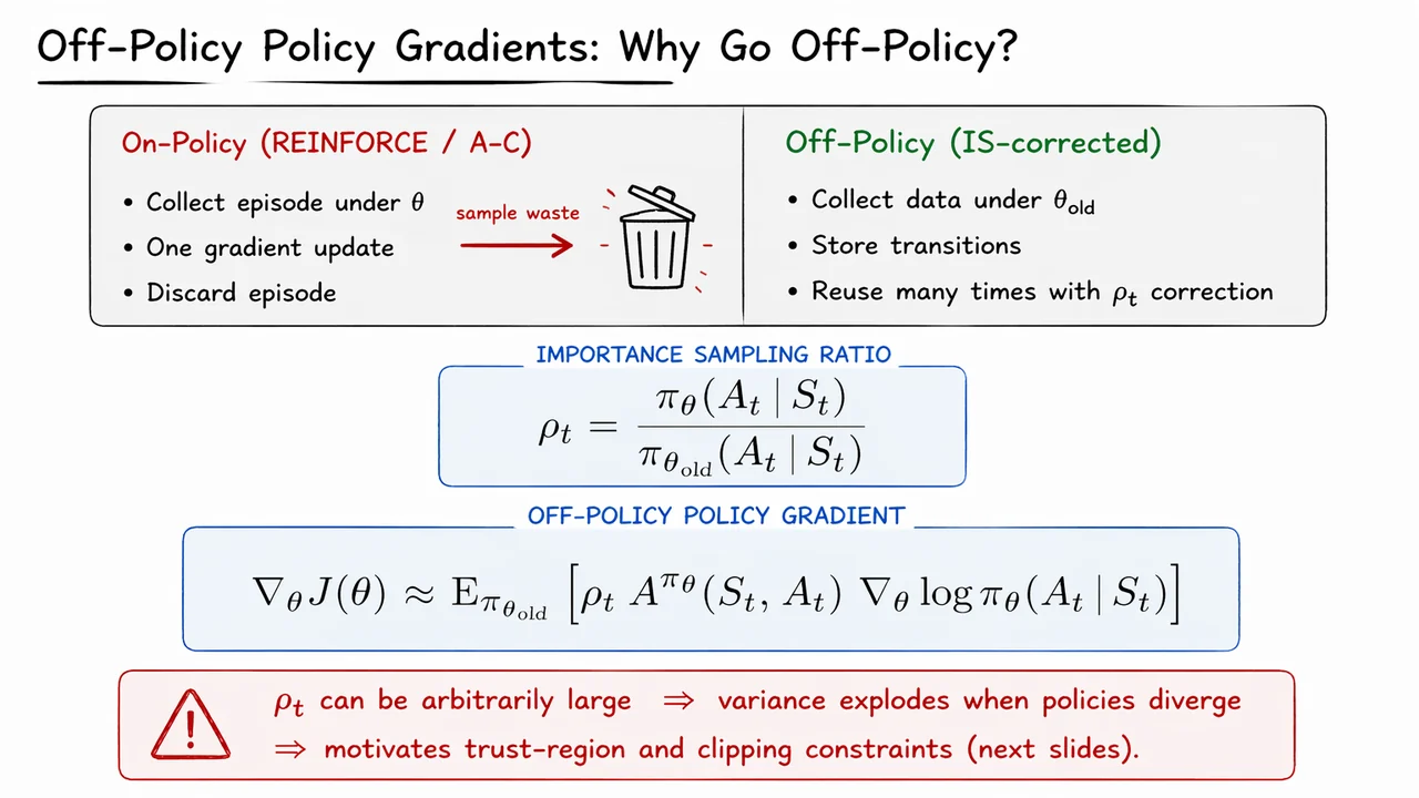
After introducing the instability of unconstrained importance weighting, the central question becomes: how do we move the policy enough to improve it, without moving so far that the old data stops being trustworthy? PPO answers this by replacing a hard trust-region constraint with a softer surrogate that behaves like a trust region where it matters most. The key object is the importance ratio which is exactly at the on-policy starting point . If the new policy increases the probability of an action that turned out to be good, ; if it suppresses a bad action, . In principle this is just ordinary off-policy correction. In practice, however, the ratio can drift too far from , and then the estimator starts to amplify noise instead of improving the policy.
PPO’s insight is not to eliminate the ratio, but to refuse to reward changes that are too extreme. The clipped surrogate objective implements this idea with a simple trick: once leaves the interval , the objective no longer gives you additional gain for pushing it farther out. That is the crucial design choice. PPO is not merely penalizing large deviations; it is removing the gradient incentive to continue in the risky direction.
The behavior depends on the sign of the advantage. If , then the sampled action was better than the baseline, so increasing its probability is desirable—but only up to a point. Beyond , the gain is capped, which prevents the update from over-committing to a possibly lucky sample. If , the action was worse than the baseline, so decreasing its probability is desirable—but again only within reason. Once drops below , the objective stops rewarding further suppression, which prevents the optimizer from “over-correcting” based on noisy negative evidence.
This is why PPO is often described as a proximal method: it encourages updates to stay near the previous policy, not through an explicit constrained optimization problem, but through the geometry of the surrogate itself. Compared with a KL-constrained formulation, this is much easier to implement and tune. Instead of solving a delicate constrained problem each iteration, we optimize a plain loss and let clipping act as a built-in safeguard. The result is a practical compromise:
A useful way to see the mechanism is to think of as a control knob. For positive-advantage samples, the unclipped objective grows linearly with , but the clipped version flattens after . For negative-advantage samples, the mirror-image effect occurs on the low side: the objective flattens before becomes too small. In both cases, the optimizer is allowed to move toward better behavior, but it is denied extra incentive to keep pushing once the policy has already departed “enough” from the old one. That subtle asymmetry is what makes clipping stable: it does not forbid change, it just caps the benefit of extreme change.
The full PPO objective also includes an entropy bonus, which nudges the policy to remain somewhat stochastic. This matters because clipping alone can make the policy too conservative, especially early in training or in sparse-reward settings. The entropy term counterbalances premature collapse by preserving exploration, while the clipped surrogate keeps that exploration from turning into destructive drift. In practice, this combination is one of the reasons PPO became the default policy-gradient workhorse in many modern deep RL systems.
The visual below condenses exactly this logic into two complementary views. The left panel lays out the three equations in sequence: the ratio , the clipped surrogate , and the final objective with entropy regularization. Read top to bottom, they show how a plain importance-weighted update becomes a stabilized optimizer. The right panel makes the more important geometric point: once crosses the band , the clipped objective goes flat in the direction that would otherwise keep increasing the update magnitude. That flat region is the mechanism behind PPO’s stability.
So the figure is not just a summary of formulas; it is a compact proof-by-picture of the main design principle. PPO keeps the benefits of off-policy correction from , but it removes the incentive to exploit that correction too aggressively. That is why it works so well in practice: it turns a fragile importance-weighted update into one that is, in effect, self-limiting.
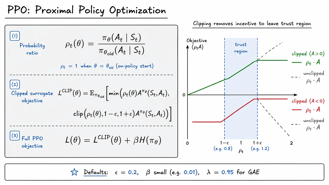
After deriving policy gradients in the abstract, the next question is almost always practical: how do we make the update stable enough to reuse data without drifting too far from the policy that generated it? PPO answers this by turning policy improvement into a controlled local optimization problem. Instead of optimizing the raw advantage-weighted likelihood ratio everywhere, it keeps a reference policy fixed, measures how much the new policy has moved via and then limits how much that ratio can help or hurt the objective.
The central subtlety is that the policy gradient wants to increase the probability of actions with positive advantage and decrease it for negative advantage, but unconstrained reuse of the same batch can make those updates explode. If , then increasing seems good in the surrogate objective, but after a point the optimizer can keep pushing even when the resulting policy is already too different from the data-collecting policy. PPO’s clipped objective is a practical compromise: This is not a hard trust region, but it behaves like a soft safety rail. Once the ratio crosses the interval , the clipped term stops the objective from rewarding further movement in that direction.
There is a nice asymmetry hidden here. When , the objective rewards increasing only until the upper clip boundary; when , it rewards decreasing only until the lower boundary. So the clipping is not merely “regularization” in the vague sense; it is specifically designed to truncate the incentive for destructive policy shifts while preserving the first-order direction of improvement around the current policy.
PPO is also not just an actor update. In the standard implementation, the algorithm jointly trains a policy network and a value network. The critic is fit by regression, and the whole system is optimized together with entropy regularization: The negative sign in front of is easy to miss but conceptually important: we are still doing gradient descent in the implementation, even though the policy term itself is a maximization objective. The entropy bonus adds another useful pressure, discouraging the policy from collapsing too early into near-deterministic behavior.
A second key ingredient is the use of generalized advantage estimation. PPO typically computes from temporal-difference residuals, then forms an exponentially weighted sum of future residuals. This gives a smoother bias-variance tradeoff than pure Monte Carlo returns or one-step TD, which matters because the clipped objective is only as good as the advantage signal feeding it. In practice, the advantages are also normalized across the batch: That normalization does not change the direction of the update in any essential way, but it makes the gradient scale much more predictable across tasks and reward magnitudes.
The training loop itself is what makes PPO sample-efficient. We first collect a batch of trajectories with the current policy, then freeze and reuse that batch for several minibatch epochs. This is the crucial compromise between on-policy purity and practical efficiency: we are still optimizing against data generated by a policy close to the one being updated, but we amortize the cost of environment interaction by taking multiple gradient steps per batch. The frozen reference policy is also what makes well-defined during those inner epochs; without that freeze, the denominator would drift underneath us and the clipped objective would lose its meaning.
That combination of ingredients is exactly what the compact pseudocode below is meant to summarize. The visual below makes the training loop feel like a pipeline: collect data, compute GAE advantages, normalize them, then repeat several minibatch passes over the same batch while the old policy stays fixed. The highlighted lines separate the roles cleanly: freeze the behavior policy, compute clipped surrogate loss, fit the value baseline, add entropy, and descend on the total objective.
The small design-choice callouts are especially useful because they point to the algorithmic reasons PPO works in practice, not just the formula itself. In particular, the diagram reinforces four ideas that are easy to forget when reading equations in isolation:
Taken together, PPO is best understood as a carefully engineered middle ground: it borrows the sample reuse of supervised optimization, the low-variance learning signal of actor-critic methods, and just enough conservatism to avoid the brittle behavior of naive policy gradients.
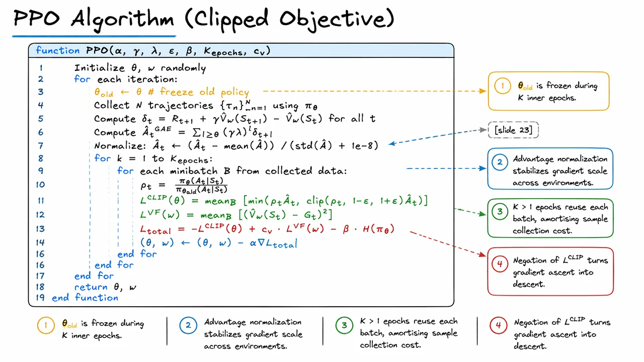
Now that PPO has been derived as a trust-region-style policy gradient with clipped importance ratios, the natural question is whether these extra ingredients actually matter in practice. The answer is yes—and the most revealing way to see it is not through another algebraic manipulation, but through learning curves under a fixed environment budget. In continuous-control benchmarks like HalfCheetah-v2 and Hopper-v2, sample efficiency is the real currency: if an algorithm needs many more interactions to reach the same return, then the optimization trick is not merely elegant, it is practically decisive.
To interpret the comparison correctly, it helps to remember what each method is buying you. REINFORCE uses Monte Carlo returns directly, so every update is an unbiased but noisy estimate of the policy gradient. That noise is especially damaging in high-dimensional continuous-control tasks, where a single bad rollout can dominate the update. Adding a baseline reduces variance by centering the return, but it does not change the fact that the signal still comes from full-trajectory outcomes. A2C goes further by using a learned critic , replacing high-variance returns with a bootstrapped advantage estimate. And PPO layers on a conservative update rule that prevents large policy shifts from destroying the data you just collected.
The key difference, empirically, is that these improvements compound rather than merely add. In the tabulated results, plain REINFORCE barely gets off the ground in HalfCheetah within one million environment steps, hovering around a return of only a few hundred. The baseline version improves this substantially, but still remains far behind actor-critic methods. A2C brings the curve into a regime where learning becomes visibly useful, reaching roughly on HalfCheetah. PPO then pushes much further, approaching under the same budget. That is not a small constant-factor improvement; it is the signature of an optimizer that can both extract more learning signal per sample and reuse data more effectively.
A useful way to think about PPO is that it solves a delicate tension in policy optimization. On the one hand, you want to reuse a batch multiple times so that each environment step contributes more gradient information. On the other hand, aggressive reuse can make the policy drift too far from the behavior that generated the batch, which breaks the assumptions behind the gradient estimate. PPO’s clipped objective limits how much a single advantage estimate can benefit from a large ratio , where This is exactly why multi-epoch minibatch reuse works: you can revisit the same data times, but the clipped surrogate keeps the update from becoming reckless. In practice, that lets PPO translate each batch into more useful parameter movement than a one-pass method like A2C.
The benchmark also highlights a subtle but important failure mode of high-variance gradients: poor early exploration can become self-reinforcing. In HalfCheetah, REINFORCE often fails to discover consistently better actions before the budget is exhausted, so the return curve stays nearly flat. The entropy bonus helps here by discouraging premature collapse to a nearly deterministic policy, keeping the optimizer willing to explore while the value estimates are still noisy. That matters most in the first few hundred thousand steps, when a brittle policy can lock the agent into a bad region of parameter space.
The practical lesson is not that PPO is magical, but that the pieces introduced earlier are doing very specific jobs:
Seen together, these explain why PPO achieves roughly the A2C return on HalfCheetah and reaches near-optimal Hopper performance in about half the steps. The point is not merely that PPO “wins,” but that it wins for the exact reasons the theory predicts: lower variance, controlled policy drift, and better sample reuse.
The visual below condenses that story into one glance. The left panel turns the learning dynamics into a clear ranking: the red REINFORCE curve stays low, the baseline version climbs somewhat, A2C rises more reliably, and PPO accelerates sharply toward the top of the return range. The vertical marker emphasizes that PPO reaches strong performance much earlier in the budget, which is the essence of sample efficiency.
The right panel complements the curve with a compact numerical summary and a short reminder of the crucial hyperparameters . Read together, the plot and table serve as empirical evidence for the earlier derivation: the clipped objective is not just a theoretical safeguard, it is what makes multi-epoch policy gradient updates work well enough to dominate the simpler REINFORCE and A2C baselines in MuJoCo.
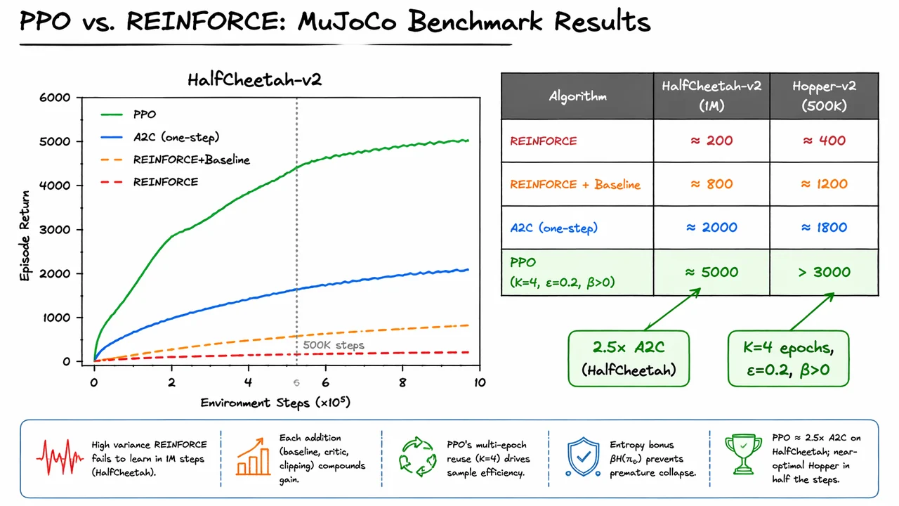
After the abstract derivation of the policy gradient, it is useful to ground the machinery in the simplest possible controlled setting: a one-step bandit. Here there is no state evolution, no credit assignment across time, and no discount factor to complicate the picture. The entire reinforcement learning problem collapses to choosing one action from , receiving a fixed reward, and updating the policy so that better actions become more likely.
This is exactly why the bandit is such a good sanity check for REINFORCE. If the score-function estimator is correct, then in expectation it should push probability mass toward the action with the largest reward and away from inferior alternatives. In other words, we want the gradient to be aligned with what we already know from the reward structure: Because the environment is so simple, we can inspect the gradient algebraically and verify that the update is not just plausible, but exactly right.
We parameterize the policy with a softmax over logits : At initialization , the policy is uniform: This symmetry makes the first update especially transparent. Since the policy starts with no preference, any change must come purely from reward-weighted gradient information.
The key identity is the softmax score function: This formula is the engine behind REINFORCE. It says that if action was sampled, then the selected log-probability is pushed up, while all logits are adjusted through the normalization term. The actual direction of the update is determined by the reward attached to that sampled action. High-reward samples reinforce themselves; low-reward samples get suppressed.
At the uniform initialization, we can compute the expected gradient exactly. For , So the lowest-reward action gets a negative push. For , So the best action gets a positive push. That sign pattern is the whole story: increase the logit of the good action, decrease the logit of the bad one.
With a small learning rate, say , the REINFORCE update is just Even from a perfectly symmetric starting point, the expected effect is already asymmetric: increases, decreases, and the policy shifts probability mass toward . This is a tiny example, but it contains the core intuition of policy gradients: sampling an action, observing its return, and nudging the policy in proportion to reward is enough to improve expected performance.
Of course, this toy setting also hints at the main weakness of vanilla REINFORCE. In a bandit, the return is immediate and noise is limited; in long-horizon problems, the same estimator can have very high variance because every sampled trajectory must carry the learning signal. That is why later variance-reduction tools matter so much: a baseline can center the return without changing the expected gradient, and actor-critic methods can replace full Monte Carlo returns with lower-variance bootstrapped estimates.
The visual below compresses this entire verification into one glance. The left side lays out the setup, the softmax policy, the score-function identity, and the two gradient calculations that certify the update direction. The right side turns those equations into geometry: before learning, the policy is uniform; after one REINFORCE step, mass moves away from and toward , exactly matching the reward ordering.
That before/after comparison is more than a picture of arithmetic. It is a concrete confirmation that the likelihood-ratio gradient estimator is doing the right thing. In the simplest possible environment, REINFORCE does not merely produce a plausible heuristic update—it verifiably pushes the policy in the direction predicted by the theorem, which is the right foundation before we move on to variance reduction on harder tasks.
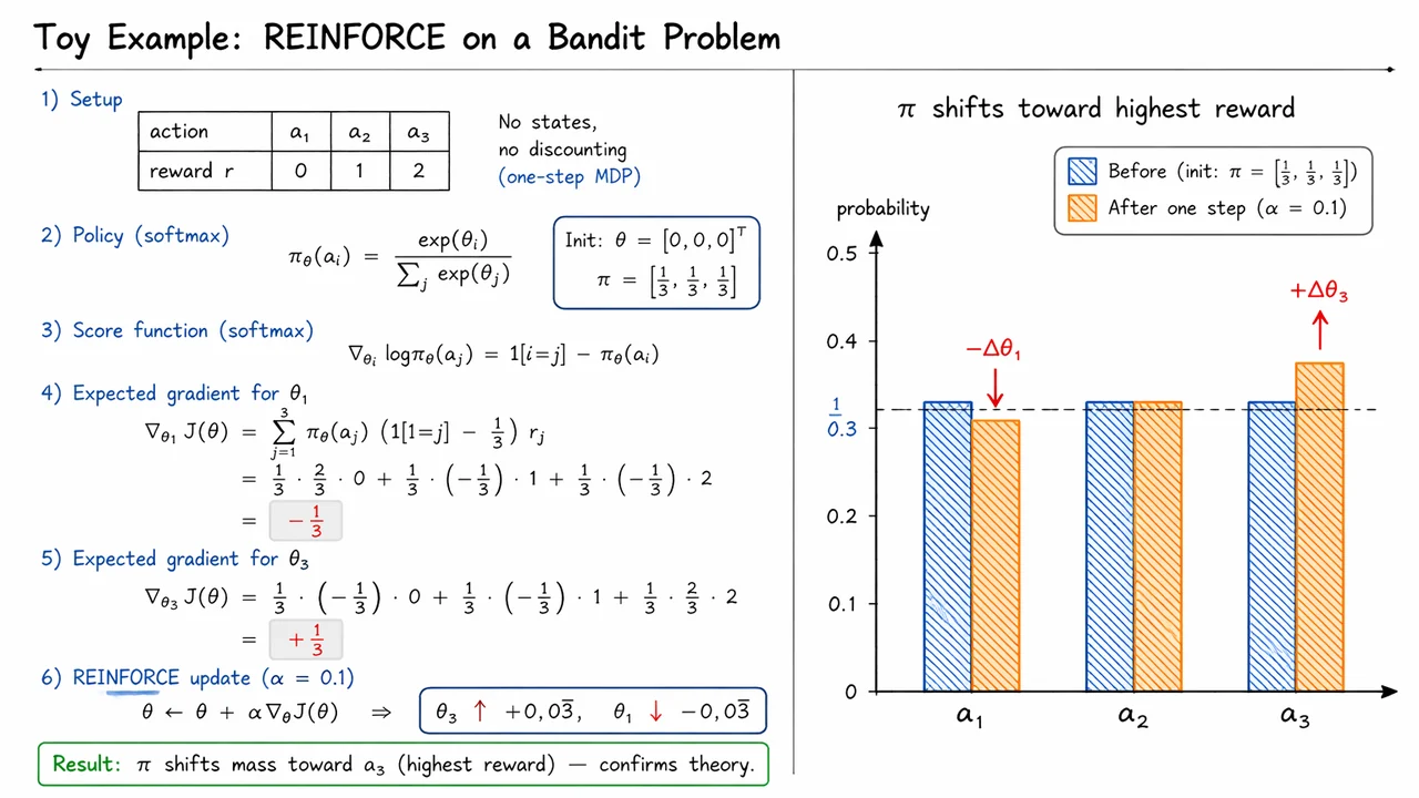
After the theory, the most convincing question is practical: does variance reduction actually change learning behavior, or is it just algebraic convenience? CartPole is a good stress test because it is simple enough to train quickly, yet still exposes the pathologies of Monte Carlo policy gradients. The task has a hard ceiling at return , so improvements are easy to interpret, and instability is immediately visible when a method overshoots or collapses.
The central issue is that the REINFORCE update uses a noisy estimate of long-term return. In its simplest form, the gradient estimator at time is proportional to
where is a Monte Carlo return. This estimator is unbiased, but in finite data regimes its variance can be so large that a single unlucky trajectory can push the policy in a destructive direction. In control problems like CartPole, that means a policy can appear to be improving and then abruptly forget what it learned because the update step was dominated by noise rather than signal.
A baseline changes that picture without changing the mean gradient. If we subtract any state-dependent baseline , the policy gradient remains unbiased because In practice we choose , the learned value function, because it approximates the expected return from that state. The quantity that matters is the advantage-like residual : it is smaller, less heteroskedastic, and therefore much easier to optimize. This is exactly why The subtle assumption here is that the baseline should not depend on the sampled action, otherwise the cancellation property breaks and bias can creep in.
Actor-critic methods go one step further by replacing the full Monte Carlo return with a bootstrapped target. Instead of waiting for the episode to finish, we form the one-step temporal-difference error This estimate is noisier in a different way: it introduces a small bias because is itself imperfect, but it dramatically reduces variance and makes updates available after every transition. In effect, the critic supplies a moving local estimate of “how much better than expected this action was,” while the actor uses that signal to adjust the policy. The tradeoff is classic: Monte Carlo is unbiased but noisy; bootstrapping is slightly biased but much more sample-efficient.
These ideas explain the empirical hierarchy we see in CartPole. Each successive method is not merely “more sophisticated”; it changes the noise properties of the gradient enough to shift the learning dynamics. A sensible summary is:
The visual below condenses that story into one plot. The curves are not just performance traces; they are evidence for the variance argument. The red REINFORCE trajectory rises erratically and even exhibits catastrophic forgetting, where a promising policy is suddenly destroyed by a high-variance update. The orange, blue, and green curves progressively narrow that instability, matching the theoretical expectation that better estimators should produce smoother optimization.
Just as importantly, the plot makes the practical meaning of variance reduction unmistakable. The baseline does not merely improve the final number; it changes the time to reach competence. The actor-critic line shows that bootstrapping can accelerate learning substantially, and PPO’s tight, flat curve reflects what happens when policy updates are additionally constrained to stay near the previous iterate. In other words, the diagram is a compact empirical summary of the same chain of reasoning we built analytically: reduce gradient variance, preserve useful signal, and optimization becomes both faster and safer.
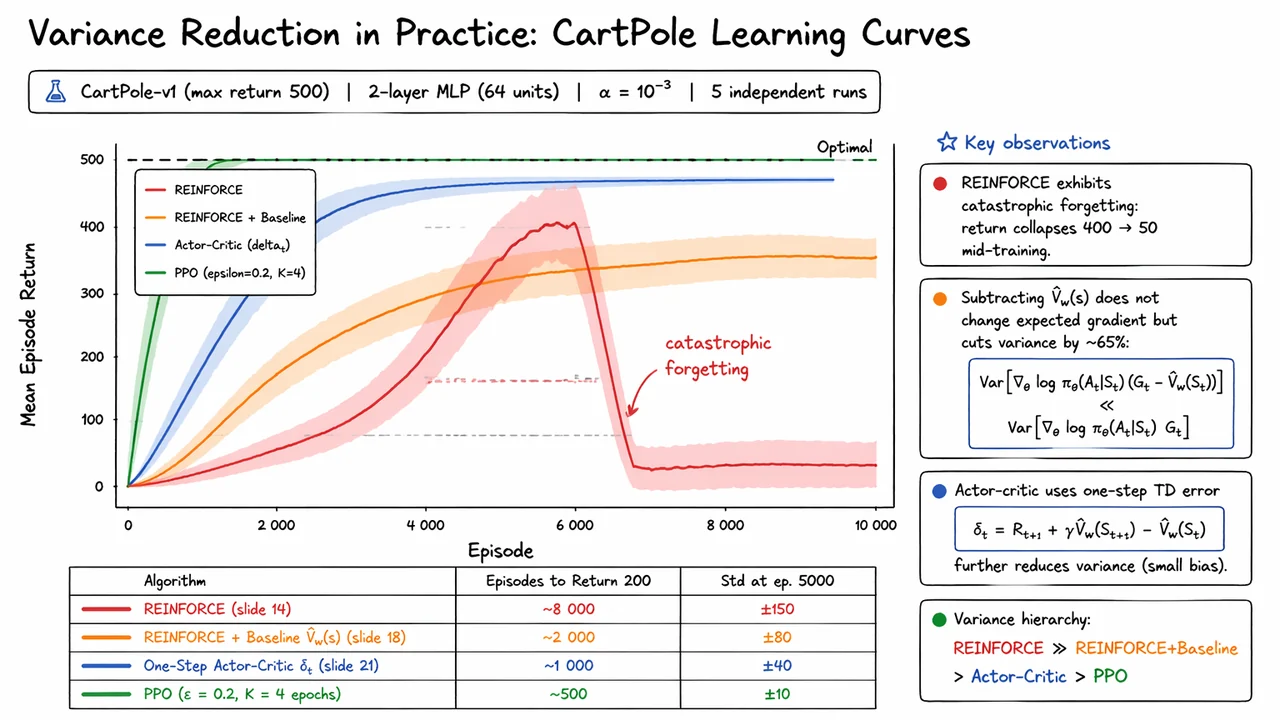
After working through REINFORCE, baselines, actor-critic updates, and their more practical descendants, the key realization is that these are not separate algorithms so much as different choices of the same estimator template. That is the unifying perspective that makes the policy-gradient literature feel much smaller than it first appears.
At the core, we optimize an objective by nudging parameters in the direction This identity is powerful because it isolates the moving parts. The policy-gradient term is always the same: it tells us how to increase the probability of the sampled action under the current policy. All of the algorithmic variation is hidden inside the scalar or vector signal , which tells us how much that action should be reinforced or suppressed.
The simplest case is Monte Carlo REINFORCE, where , the full return This choice is unbiased, but it is also notoriously noisy. The return depends on every random reward that follows the action, so the credit assigned to a single decision can fluctuate wildly from episode to episode. That is mathematically acceptable, but statistically inefficient: the estimator has to average out a lot of variance before the true direction becomes visible. In long-horizon problems, that can make learning painfully slow.
A baseline changes the story without changing the expectation. If we replace with , and the baseline depends only on the state, the gradient remains unbiased because the policy-gradient term has zero mean under the current policy. Intuitively, we are not changing what is good or bad, only re-centering the signal around what we already expect from that state. This is an important subtlety: variance reduction is not the same as changing the objective. The baseline removes predictable structure, leaving the update focused on the action-specific surprise.
Actor-critic methods push this idea further by replacing Monte Carlo return estimates with a learned critic. The one-step temporal-difference error is a much cheaper learning signal than a full return. Its advantage is immediate: it can be computed online, before the episode ends, and it typically has much lower variance. The price is that is only an approximation to , so the update can become biased if the critic is inaccurate. In practice, this trade-off is usually worthwhile because a slightly biased but stable direction often learns faster than an unbiased but chaotic one.
There is a spectrum here, not a binary choice. -step actor-critic interpolates between full Monte Carlo and one-step TD by mixing real returns with bootstrapping, while GAE forms a weighted sum of TD errors, The parameter is the knob that controls how much we trust long-horizon Monte Carlo evidence versus short-horizon critic bootstrapping. Small leans toward low variance and stronger bias from the critic; large leans toward more accurate but noisier advantage estimates. This is why GAE is so widely used: it exposes a principled bias–variance continuum rather than forcing a hard choice.
PPO fits into the same framework, but with an extra layer of conservatism. Its clipped objective uses an advantage estimate, usually from GAE, but prevents the new policy from moving too far in one update through an importance ratio and clipping. That makes the overall method more stable and sample-efficient, especially when function approximation and multi-step bootstrapping interact. The important thing is that even here, the gradient is still being driven by a shaped version of ; the machinery around it mainly manages update size and off-policy drift.
So the unifying lesson is simple but deep:
The visual below condenses exactly this perspective. The top equation identifies the common template, while the table organizes the major algorithms by the one thing that really changes: the choice of . Once that is clear, the color pattern becomes meaningful rather than decorative: green is not “better” in an absolute sense, but a reminder that low variance often comes from learned structure, and learned structure is where approximation error can enter.
Read the table as evidence for the principle we have been building toward: policy-gradient methods are unified by the same estimator form, and their practical differences come from how they trade bias, variance, and sample efficiency through the design of .
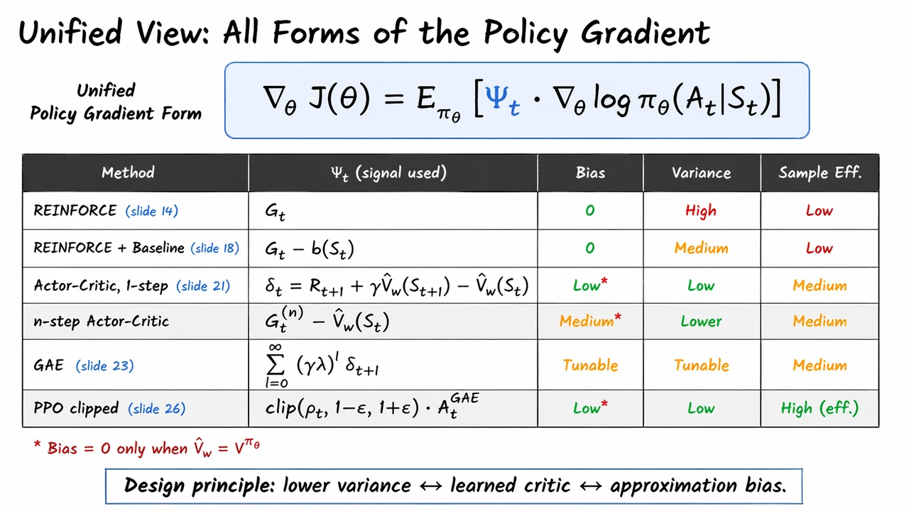
When we first learn reinforcement learning, it is tempting to imagine that the hardest part is estimating a good value function and then simply acting greedily with respect to it. That works beautifully in discrete problems with a small action set: learn , choose , and you have a policy. The logic is elegant because it reduces control to prediction.
But that elegance hides an important assumption: that the action space is easy to search, that one action is enough to represent the right behavior, and that the agent can truly observe the relevant state. Once any of those assumptions breaks, a value function alone becomes a brittle intermediary rather than a solution.
The greedy policy induced by a value function is typically written as This expression is harmless when is finite and small. In that case, the argmax is just a comparison over a short list. But if , the expression quietly becomes a nested optimisation problem: every time the agent wants to act, it must solve a continuous maximisation over actions. For high-dimensional control, that is not a small implementation detail — it is the central computational bottleneck.
That is the first failure mode: continuous actions. Here, the issue is not that -learning is conceptually wrong, but that the greedy extraction step is no longer cheap. We are no longer choosing among a handful of actions; we are searching over an uncountable space. Unless the critic has a special structure, is itself a hard optimisation problem, and we have merely moved the difficulty from policy learning into action selection.
The second failure mode is more subtle: perceptual aliasing. Imagine two different underlying situations that produce the same observation. From the agent’s perspective, the states are indistinguishable, but the correct behavior may differ. A deterministic greedy policy must commit to one action per observation, yet the best response may require a mixture over actions. In that case, the policy needs to encode uncertainty or ambiguity directly: A stochastic policy can represent “sometimes go left, sometimes go right” in a principled way; a pure argmax policy cannot.
This distinction matters because the right response is not always “pick the single best action.” When two hidden states collapse to the same observation, the agent may need to randomize to average over incompatible optimal actions. In other words, the policy is not just a decision rule; it is part of the model of how the agent resolves ambiguity.
The third failure mode is partial observability, where the agent does not directly observe the full Markov state at all. In a POMDP, the observation history or belief state is what matters, and deterministic policies can be fundamentally suboptimal. Stochasticity is not merely a convenience here — it can be structurally necessary, and there are settings where the best deterministic policy performs arbitrarily badly compared with a stochastic one. This is one of the most important conceptual reasons to stop treating “policy = argmax over value” as the universal template.
So the real lesson is not “value functions are useless.” Rather, value functions are often the wrong interface for control. If the action space is large or continuous, or if the environment forces the agent to randomize, then the policy itself should be optimized directly. That is exactly what policy gradient methods do: instead of first learning a value surface and then extracting a policy by maximization, we parameterize the policy and improve by following the gradient of expected return.
The visual below compresses these three failure modes into one glance. The left panel emphasizes that in continuous action spaces, the obstacle is the search problem hidden inside . The middle panel shows why aliased observations can demand a mixed strategy, making a stochastic policy strictly more expressive than a deterministic one. The right panel captures the POMDP intuition: when the agent does not fully observe the state, stochastic policies can outperform any fixed deterministic rule.
Taken together, the three panels justify the move that policy gradient methods make from the start: rather than asking how to recover a policy from a value function, we ask how to optimize the policy directly. That shift is what makes the rest of the lecture possible — from the likelihood-ratio derivation to REINFORCE, baselines, and actor-critic methods.
We now want a failure case that is simple enough to reason about in one glance, but rich enough to expose the real limitation of value-based control. The key idea is perceptual aliasing: the environment may be fully Markov in the underlying state, yet the agent’s observation collapses several distinct states into the same feature vector. Once that happens, the policy no longer gets to condition on the true state, only on what it can see.
That distinction matters because a value method such as Q-learning ultimately extracts a deterministic control rule, so every observation is mapped to a single action. If two or more hidden states share the same observation but require different actions, then a deterministic policy is forced to “average over” incompatible choices by committing to one of them. In a standard MDP with full observability, that is usually fine; in an aliased setting, it can be fatal.
A small gridworld makes the issue concrete. Imagine a grid with a goal in one corner and four interior squares that all look identical locally: each has walls on the same two sides, so the agent sees the same feature vector in all four places. The true state differs, but the observation does not. From the agent’s perspective, these are not four distinct situations — they are one ambiguous observation repeated in four locations.
Now ask what a deterministic policy can do. Because it must output a single action for the shared observation, it must choose the same move in each aliased square. But no single move is simultaneously correct everywhere: an action that escapes one hidden configuration may hit a wall or send the agent into a loop in another. In this kind of construction, any fixed choice incurs a substantial failure probability, and the expected return stays low. The problem is not that the policy is poorly trained; the problem is that the policy class is too rigid.
A stochastic policy is different in exactly the right way. Instead of collapsing the decision to one action, it can represent a distribution or symmetrically over , so that the agent randomizes between two perpendicular escape directions. This is not indecision for its own sake; it is a principled response to partial observability. When the same observation corresponds to several hidden states, randomization can hedge against the hidden ambiguity and produce a much higher return than any deterministic commitment.
This is exactly why the usual greedy value-based view can break down here. The maximizer assumes that one action should dominate for the state under consideration. But when the observation aliases multiple hidden states, the induced greedy policy is still deterministic and therefore cannot adapt to each hidden case separately. Even if the Q-function is accurate with respect to the underlying hidden dynamics, the final policy extraction step throws away the very stochasticity that would solve the task.
The broader lesson is that we should optimize the policy directly, not merely infer it indirectly from values. By parameterizing and maximizing , we allow the model class itself to include useful stochastic strategies. That is the real motivation for policy gradients: they are not just another way to train controllers, but a way to learn policies whose distributional structure is essential to success.
The visual below compresses this argument into two contrasted worlds. On the left, the deterministic controller is trapped by a single committed action: the same red arrow must serve every aliased square, so at least some hidden cases fail or cycle. On the right, the stochastic policy assigns probability mass to multiple actions, and that extra flexibility lets the agent escape the ambiguous region and reach the goal with high probability.
If you keep one idea from this example, let it be this: when the observation is ambiguous, the right object to learn is not just a value function, but a parameterized policy distribution. This is the conceptual bridge from “why not just learn a value function?” to the policy-gradient objective that follows.
After the failure modes of aliasing, the next question is almost unavoidable: what exactly are we optimizing when we say “learn a policy”? In policy gradients, the answer is not a value table or a greedy action rule, but a parameterized stochastic policy whose parameters can be adjusted by gradient ascent. Formally, at each time , the policy defines a distribution over actions, so the policy is not a single action choice but a family of action probabilities that can be made sharper, smoother, or more exploratory depending on .
The objective in episodic reinforcement learning is to choose so that trajectories with high long-term return become more likely. A standard way to write this is where is the discounted return from the start of an episode. This is already useful conceptually: instead of optimizing immediate reward, we optimize the expected total outcome under the policy’s own behavior. If the initial state is random, we can also view this as an average over the initial-state distribution : This makes the dependence on the policy explicit through the value function , while separating it from the environment’s starting-state distribution.
It is often cleaner to reason not at the level of states, but at the level of entire trajectories. A trajectory is a full episode sampled from the policy and the environment dynamics, and the same objective can be written as This trajectory view is the one that later makes the likelihood-ratio trick work. It turns the objective into an expectation over a distribution , which is the key object we need when differentiating .
The crucial structural fact is that the trajectory probability factorizes into two very different parts: Only the policy terms depend on . The environment transition probabilities and the initial-state distribution are fixed by the environment. This distinction matters enormously: it is what makes policy gradients possible even when the dynamics are unknown, non-differentiable, or too complex to model directly. We never need to differentiate through the environment; we only need to know how the policy assigns probability to the actions it takes.
This also explains why policy-gradient methods are so different from value-based methods. Instead of solving for a greedy argmax over actions, we directly reshape the action distribution so that trajectories with larger return become more likely. In that sense, the optimization problem is:
That update rule is deceptively simple, because the real challenge is estimating from sampled experience. But once the objective has been written at the trajectory level, the path to REINFORCE and the policy gradient theorem becomes natural: we will differentiate an expectation over trajectories, isolate the -dependent policy factors, and turn return-weighted action probabilities into a usable learning signal.
The visual below compresses exactly that logic. The left side collects the same objective in three equivalent forms: policy, state-value, and trajectory expectation. That progression is not redundant; it shows that we can move between local decisions and global episode performance without changing the underlying quantity we optimize. The final boxed update rule at the bottom is there to remind you that all of this structure ultimately feeds one operation: gradient ascent on .
On the right, the unrolled trajectory diagram reinforces the most important modeling asymmetry: the blue arrows are controlled by , while the gray arrows belong to the environment. That is the conceptual hinge of policy gradients. We are not trying to redesign the world; we are only adjusting how the agent samples actions inside it.
After introducing the policy objective, the next question is not why we would optimize a stochastic policy, but how we can take gradients of it in a form that is actually usable. The key object is the score function : once this quantity is available, the policy gradient machinery becomes concrete, because the gradient of the return can be written as an expectation of that score weighted by advantage-like signals.
The point of this section is that two standard policy classes give us exactly the kind of differentiable structure we need. They look different—one for discrete action spaces, one for continuous action spaces—but both produce a clean log-derivative that can be computed by ordinary backpropagation. That is the crucial bridge between abstract policy optimization and implementable algorithms.
For a discrete action set, the most common choice is the softmax policy. If we assign each action a feature vector , then the policy is This is just a normalized exponential family model over actions: the numerator prefers actions whose features align with , and the denominator ensures the probabilities sum to one. The shape of the resulting gradient is especially elegant: In words, the update direction is the observed feature vector minus the policy’s own expected feature vector. That centering matters: it prevents the gradient from simply chasing large feature magnitudes and instead measures how surprising the chosen action was relative to the current policy. This is one reason softmax policies behave so naturally in REINFORCE-style updates.
For continuous actions, the canonical choice is a Gaussian policy. Instead of selecting an action from a finite set, the policy outputs a mean and samples around it: Here the policy class is smooth in the parameters through the mean network , and the score function becomes This expression is extremely informative. The scalar factor says that actions sampled above the mean and below the mean push the network in opposite directions, with larger deviations creating stronger learning signals. The vector factor is where standard backpropagation enters: once the mean is represented by a neural network, the policy gradient can be propagated through it exactly like any other differentiable model.
A useful way to compare the two cases is:
This smoothness is not a cosmetic detail. Policy gradient theory relies on being able to exchange differentiation and expectation, so the parameterization must be well-behaved enough for the gradient of to pass through the stochastic action selection. Softmax and Gaussian policies are the workhorses because they satisfy this requirement while still remaining simple enough to evaluate and differentiate exactly.
The visual below condenses that story into two parallel pipelines. The left panel captures the softmax case as “scores probabilities centered features,” while the right panel shows the Gaussian case as “mean network density backpropagated score.” Read together, they reinforce the main lesson: the policy gradient method does not need to differentiate through the sampling operation itself; it only needs a policy class whose log-derivative is tractable.
That is why these two parameterizations appear so early in the policy-gradient story. They are not merely convenient examples; they are the concrete templates from which REINFORCE, baseline methods, and actor-critic algorithms all inherit their gradient estimates.
Having defined a policy class, the next question is not what to optimize, but how to differentiate the objective efficiently. In policy gradient methods, we want to maximize
where denotes an entire trajectory and is the return accumulated along it. The key subtlety is that does not appear inside the reward function itself; it appears in the distribution over trajectories. That means the objective is an expectation whose measure depends on the parameters we are trying to optimize. This is exactly the kind of situation where naive differentiation becomes awkward.
If we write the gradient directly, we get
At first glance, this looks like something we might pass through the integral sign. But that instinct hides the real difficulty: the integrand is not just , it is times a parameter-dependent density. The domain of integration over trajectories does not move, but the probability mass assigned to each trajectory does. So the challenge is not “differentiate the reward”; it is “differentiate through the sampling distribution that generates the data.”
This distinction matters because in reinforcement learning, the return is often noisy, delayed, and discontinuous with respect to actions. There is usually no differentiable computational graph from to in the way that standard backpropagation assumes. Instead, the policy influences the likelihood of seeing different trajectories:
Here the environment dynamics and initial-state distribution are typically fixed, while the policy is the only factor that changes with . This is the source of the gradient signal—but also the source of the technical obstacle. The parameter dependence is buried inside a product of probabilities, not inside a simple explicit formula for .
A tempting workaround is numerical differentiation. For the -th parameter component, one could approximate
This finite-difference estimate is conceptually straightforward, but it is computationally disastrous at scale. Each component of requires two fresh evaluations of the full objective, and each evaluation requires many rollouts because itself is stochastic. For a neural policy with millions of parameters, that means millions of full rollouts per update in the worst case. The method is therefore not just slow; it is fundamentally mismatched to large-scale RL.
The real lesson is that we need a way to convert a gradient of an expectation into an expectation of a gradient-like quantity that can be estimated from sampled trajectories. In other words, we want to keep the Monte Carlo friendliness of sampling while still obtaining a valid derivative signal. That is the conceptual bridge to the likelihood ratio trick, which will let us rewrite the gradient without differentiating through the environment or through the return directly.
A useful way to keep the three roles separate is:
The visual below condenses exactly this bottleneck. The central equation emphasizes that the gradient is acting on an expectation, while the highlighted trajectory density reminds us that the parameter dependence lives inside the measure. The finite-difference box captures the brute-force alternative and why it scales so badly, and the bottom banner previews the escape hatch: once we apply the likelihood ratio trick, the gradient becomes something we can estimate from ordinary rollouts instead of from prohibitively many reruns.
We now have the core difficulty in focus: the objective is an expectation over trajectories, but those trajectories themselves depend on the policy parameters . That means the derivative is not just acting on a familiar integrand ; it is acting on the distribution . In other words, the obstacle is measure-theoretic rather than algebraic. If we try to differentiate the return directly through the environment, we immediately run into the fact that the dynamics may be unknown, discontinuous, or simply not differentiable in any useful way.
The key move is to rewrite the gradient in a form that isolates the parameter dependence inside a logarithm. For any differentiable density or mass function , the log-derivative identity says
This is just the chain rule in disguise: , so multiplying through by recovers the original gradient. The point of this identity is not aesthetic; it is operational. It turns an awkward derivative of a probability measure into something that looks like an ordinary expectation under the same distribution.
Applying it to the return objective,
we obtain
So the gradient is
This is the essential policy-gradient transformation: the difficult derivative of an expectation becomes an expectation of a score function, i.e. the gradient of the log probability. Once written this way, the gradient can be estimated by Monte Carlo rollouts from the current policy, without differentiating through the environment’s state transitions.
A few subtle points are worth keeping in mind. First, this identity does not make the estimator low-variance by itself. In fact, the raw term is often noisy because the return can fluctuate wildly across trajectories. That is why later we will introduce baselines and advantage functions: they preserve the expectation while reducing variance. Second, the derivation assumes we can exchange gradient and integral under mild regularity conditions; in practice this is usually justified for the smooth parameterizations used in policy networks, but it is still an assumption hiding in the background.
Conceptually, the result matters because it gives us a way to optimize policies in environments where the dynamics are unknown, stochastic, or non-differentiable. The only thing we need to differentiate is the policy’s own log-probability, which is exactly what neural networks can provide. That is why the score-function form is the foundation of REINFORCE, of baseline methods, and eventually of actor-critic algorithms. All of those methods are variations on this same expectation identity.
The visual below compresses that logic into a compact typographic progression. The top reminder isolates the original problem: the gradient is acting on a -dependent measure. The middle identity box captures the whole trick in one line, with the short chain-rule proof underneath to show that nothing mysterious is happening. The bottom derivation then walks from the original integral to the Monte Carlo-friendly expectation, highlighting the exact point where the likelihood ratio form turns a hard calculus problem into a sampling problem.
Read as a whole, the figure is less a derivation than a map of the transformation: from a derivative that seems to require environmental gradients, to a score-function expectation that can be estimated from sampled trajectories. That transition is the conceptual hinge for everything that follows.
Having established the likelihood-ratio identity, the next question is what actually sits inside the trajectory score . This is the point where policy gradients become especially elegant: the trajectory probability factors into pieces generated by the environment and pieces generated by the policy, and only one of those depends on .
For a finite-horizon trajectory , the joint density under policy is
Taking logs turns the product into a sum:
This decomposition is not just algebraic bookkeeping. It encodes a crucial modeling assumption: the environment evolves according to dynamics that do not change when we adjust the policy parameters . In other words, the policy chooses actions, the environment reacts, but the environment itself is not being differentiated through. That is exactly why the policy gradient method is called model-free: we do not need a differentiable model of the transition kernel to compute the gradient.
Now apply . The initial-state term vanishes immediately, and so do all transition terms , because they are independent of . What remains is just the sum of policy score functions:
This is the heart of the derivation. Every time step contributes a local sensitivity term saying how the log-probability of the sampled action changes if we nudge the policy parameters. The environment still shapes the trajectory, but it contributes only through the realized states and rewards, not through any explicit gradient path.
Substituting this back into the likelihood-ratio form from the previous step yields the familiar REINFORCE estimator:
A useful way to interpret this is as a correlation estimator: trajectories with larger return reinforce the action choices that produced them. The estimator is unbiased, but it is also noisy because the same scalar return multiplies every action score in the trajectory. That variance problem is exactly what motivates baselines, reward-to-go, and actor-critic methods later on.
There is also a subtle but important boundary condition here. The cancellation of relies on the standard policy-gradient setting where the environment dynamics are fixed with respect to . If the policy parameters were to influence the dynamics directly, or if we were learning a differentiable simulator model jointly with the policy, then additional gradient paths could appear. In the classical RL setting, however, the result is clean: the only differentiable object inside the trajectory probability is the policy itself.
So the conceptual message is compact:
The visual below condenses exactly that logic into three steps: expand the log trajectory probability, delete the -independent terms, and arrive at the model-free policy gradient. It is less a new derivation than a proof-of-cancellation, and that cancellation is what makes policy gradient methods practical in unknown environments.
We can now make the policy gradient estimator a little more honest about when information becomes available. The previous form used the full trajectory return with every score term , but that quietly mixes together rewards that happened before action with rewards that happen after it. Intuitively, that is wasteful: if a reward has already occurred, then the action at time could not have caused it.
This is where causality enters. In an MDP, action is selected after observing , and only then does the environment transition forward. So when we ask how the parameters should change to increase expected return, the only rewards that should matter for the decision at time are the ones that lie in its causal future. Past rewards are fixed by the time the action is taken, so they cannot provide a useful learning signal for that action.
Formally, the key observation is a zero-mean identity. For any reward with , the score function term has no positive correlation with that past reward: This is not saying the gradient term is literally zero everywhere; it says that, in expectation, the contribution from rewards that happened before the action cancels out. That cancellation is exactly what lets us simplify the estimator without changing its mean.
So the full-trajectory return can be replaced by the future return from time : With that substitution, the policy gradient becomes This is the causal form of REINFORCE: each action is paired only with the rewards that it could plausibly influence.
The practical benefit is important. We have preserved unbiasedness because we only removed terms whose expectation is zero. But we have also improved the estimator’s variance. Every time we multiply a score term by the full return, we inject noise from rewards that the action could never affect. Removing those irrelevant terms usually makes the gradient signal sharper and learning more stable.
There is a subtle point worth emphasizing: this is not merely a bookkeeping trick. The same return appears in every time step’s gradient estimate, but the relevant portion of that return depends on the time index. The estimator is therefore less like “score times total outcome” and more like “score times the consequences that lie ahead from this decision.” That causal interpretation is what makes the later actor-critic and advantage formulations feel natural rather than ad hoc.
A few takeaways make the logic compact:
The visual summary below organizes exactly this flow: the older full-return expression is shown as the starting point, the causal identity in the middle highlights why the past contributes nothing in expectation, and the final expression keeps only . The small timeline on the side is especially useful because it turns the abstract proof into a picture: the red region marks rewards that are already in the past and therefore dropped, while the green region marks the future rewards that remain attached to the action.
Read that diagram as a compact proof sketch. The arrows are doing the same logical work as the equations: first identify the overcounted past, then invoke causality and zero expectation, and finally arrive at the lower-variance estimator that will power the rest of the policy gradient methods we build next.
Having established why only future rewards matter, we can now strip the problem down to its cleanest possible form and see the policy gradient mechanism with almost no distractions. The one-step MDP is the smallest setting where the entire idea is already present: there is a fixed start state , we sample a single action , and then immediately receive reward . There is no trajectory credit assignment yet, no return-to-go, and no bootstrapping—just a stochastic choice followed by a scalar payoff.
In this case, the objective is simply the expected reward under the policy: This is the most direct expression of what policy optimization means. We are not trying to predict rewards explicitly; instead, we are adjusting the parameters so that the policy places more mass on actions that empirically lead to higher reward. The dependence on is entirely through the action probabilities.
The key step is to differentiate with respect to . Since does not depend on the policy parameters, it passes through the gradient unchanged: At this point the expression is correct but not yet useful, because it involves directly. The standard trick is to rewrite that derivative in terms of the log-probability: This is just the identity , sometimes called the likelihood ratio trick or log-derivative trick. Its power is that it converts a derivative of a probability into a probability-weighted derivative of a log-probability, which is exactly what we can estimate from samples.
Substituting that identity gives Now the gradient is written as an expectation under the current policy: This is the score function estimator in its most elementary form. The “score” is the gradient of the log policy, and the reward acts as the weight that says how strongly that sampled action should influence the update. High-reward actions push the policy up; low-reward actions push it down.
The intuition is worth stating carefully. Because points in the direction that increases the log-probability of action , multiplying by means:
So the gradient ascent update literally “moves probability mass” toward the better actions. This is the first place where the probabilistic interpretation of policy gradients becomes concrete: we are not editing a value table, we are nudging a distribution.
There is also a subtle but important assumption hiding here: the reward term must be independent of for this derivation to hold in this simple form. In the one-step MDP, that is naturally true because the reward is treated as a function of the chosen action and state, not of the parameters directly. In more general settings, the same idea survives, but the algebra becomes richer because the action influences future states and rewards through the trajectory distribution.
The visual below compresses this chain into a single, readable flow: from the one-step setup, to the expected-reward objective, to the log-derivative rewrite, and finally to the boxed score function estimator. Read it as a compact proof sketch rather than a standalone formula sheet—the point is not just that the identities are true, but that each line prepares the next one by turning an awkward derivative of probabilities into a sample-friendly expectation.
We can now make the score-function update feel geometric rather than merely algebraic. The key question is not just what gradient ascent computes, but how a change in parameters moves the policy itself. For a discrete action space, the policy is a probability distribution over actions, so a gradient step should be understood as redistributing mass across actions, not simply nudging numbers in parameter space.
In the one-step setting, the objective is the expected reward Applying the likelihood ratio trick gives This is already the essential geometric statement: each sampled action contributes a direction in parameter space, and that direction is weighted by how much reward followed that action. If the reward is positive, the update reinforces the probability of that action; if it is negative, the update suppresses it.
A useful way to think about this is to imagine each action carrying its own “vote” in the parameter update. The score function tells us how to increase the probability of locally, and the reward determines how loud that vote is. So the update is a reward-weighted sum of score directions, not an undifferentiated push toward every action equally.
This also explains why the update behaves sensibly in the presence of multiple actions with different payoffs. Suppose we start from a uniform policy over three actions, , with rewards , , and . Then a single gradient step should:
The important subtlety is that the policy update is relative. Because probabilities must still sum to one, increasing mass on high-reward actions necessarily takes mass away from lower-reward ones. This is why policy gradients are often described as pushing probability mass uphill on the reward landscape: the geometry lives on the simplex of categorical distributions, where improvement in one region implies contraction elsewhere.
There is also a deeper connection to reinforcement as a statistical learning principle. The update behaves like a policy-level analogue of Hebbian learning: actions that are “co-activated” with positive reward are strengthened, while actions associated with poor outcomes are weakened. Unlike supervised learning, however, the signal is not a target label; it is a scalar return that only tells us whether the sampled behavior was valuable.
Of course, this clean picture hides the fact that the raw Monte Carlo gradient can be noisy. A single sampled reward may be unrepresentative, and the score function can have large variance even when the direction is unbiased. That limitation is precisely why later variants introduce baselines and critics: they keep the same geometric rule—push mass toward better-than-average actions—while reducing the randomness in how hard each action is pushed.
The visual below compresses this intuition into a simple before-and-after story. Starting from equal probability bars, the update arrow points from the uniform policy to a new distribution where the tallest bar belongs to the highest-reward action, the intermediate reward gets a moderate increase, and the negative-reward action shrinks. The curved arrows are doing more than decorating the diagram: they encode the fact that the gradient acts like a mass transport mechanism, lifting probability where reward is high and draining it where reward is low.
Seen this way, the diagram is not just a summary of a particular example. It is a compact geometric rendering of and of the update Together, they say the same thing: policy gradients do not directly optimize actions; they reshape probability mass so that better actions become more likely.
Building on the geometric view from before, we can now state the central identity that makes policy gradients practical: the gradient of performance can be written as an on-policy expectation of a local score term weighted by an action-value signal. This is the point where the optimization problem stops looking like “differentiate through the whole environment” and starts looking like “increase the probability of actions that turn out well.”
Formally, for a differentiable stochastic policy , define the return objective as the expected value under the policy’s own visitation distribution: The notation matters here. The objective is not just a sum of per-state values; it is weighted by , the distribution over states the current policy actually visits. That dependence on is exactly what makes policy gradients seem tricky at first glance. If we differentiate naively, it looks like we should have to backpropagate through both the value function and the state distribution. The theorem says something surprisingly cleaner happens.
The policy gradient theorem states that Equivalently, using the score-function identity , we obtain the compact expectation form This is the form that powers REINFORCE and essentially every modern policy-gradient method. It says: sample from the current policy, evaluate how good the sampled action was in hindsight, and nudge the policy parameters in the direction that makes that action a little more likely.
The subtle, non-trivial part is what does not appear. Although depends on , there is no explicit term in the theorem. That omission is not a shortcut or approximation; it is an exact cancellation that follows from the dynamics of Markov decision processes. Intuitively, the effect of changing the policy on future state visitation is already accounted for indirectly through , because the action-value function captures the downstream consequences of choosing in . In other words, the theorem separates where the policy acts locally from how the environment propagates those choices forward.
This is why the theorem is so useful computationally. If the gradient had to explicitly differentiate through the visitation distribution, we would need a model of the environment dynamics or a full unrolled computation graph of the trajectory distribution. Instead, the theorem gives a model-free policy gradient that only requires sampled trajectories and estimates of or returns. It applies both to episodic tasks, where can be read as a discounted occupancy measure, and to continuing tasks, where it is the stationary state distribution.
A few implications are worth keeping in view:
This theorem is the conceptual bridge between the intuitive “push probability mass toward good actions” picture and the concrete algorithms that follow. REINFORCE will replace with sampled returns ; baselines will subtract variance-reducing terms without changing the expectation; actor-critic methods will learn a low-variance approximation to . All of those variations are easier to understand once this identity is in place, because they are all trying to estimate the same gradient in different ways.
The visual below is best read as a compact summary of that logic. The top portion collects the objective and the theorem statement in symbolic form, while the highlighted expectation form emphasizes the result we actually use in algorithms. The small notes at the bottom are there for two reasons: first, to underline that is absent despite seeming unavoidable; second, to remind us that the theorem covers both episodic and continuing settings. Taken together, the diagram condenses the whole message of the theorem: policy gradients are exact, on-policy, and local in form even though their effect is long-horizon and global in consequence.
We now have the statement of the policy gradient theorem; the remaining question is why it is true and, just as importantly, why the proof is structured the way it is. The key difficulty is that the objective depends on in two intertwined ways: directly through the policy , and indirectly through the state distribution induced by repeatedly following that policy. A naive differentiation would appear to require tracking how the entire trajectory distribution changes with , which looks hopeless.
The proof avoids that trap by working with the Bellman recursion for the value function. Starting from we apply the product rule: This split is the heart of the argument. The first term already has the shape we want: a policy gradient weighted by action value. The second term is the annoying recursive remainder, but it is also where the Bellman equation earns its keep.
To expand , write the action-value function in one-step form: The transition kernel and reward are environment properties, so they do not depend on . Only the downstream value does. Hence This is the recursive step: the gradient of the value at one state is expressed through the gradient of the value at successor states, discounted by . If you keep substituting this relation forward, the gradient propagates along all possible future trajectories, with each path accumulating a factor of and its corresponding probability under .
That recursive unrolling produces a discounted visitation-weighted sum over states: It is useful to name the discounted occupancy measure This normalization is not just a cosmetic trick: it packages the infinite unrolling into a distribution over states visited under the policy. The important subtlety is that the derivative of this distribution never has to be computed. The proof does not differentiate the state occupancy measure directly; instead, it accumulates the contributions that flow through it, which is why the theorem is so practical.
At this point, the final simplification is the log-derivative trick: Substituting this converts the gradient into the familiar expectation form, The proportionality hides the normalization constant from , but that constant is irrelevant for optimization because it does not change the direction of ascent. What matters is that the gradient can be estimated from sampled trajectories using only terms evaluated along the visited states and actions.
There are two conceptual payoffs here:
That second point is what makes REINFORCE possible, and it also explains why the estimator is so noisy: the theorem gives us a correct unbiased direction, but it does not reduce variance by itself. Baselines, advantage functions, and actor-critic methods will all be refinements of this same identity, designed to replace the raw -signal with lower-variance surrogates while preserving unbiasedness.
The visual below condenses this proof into a compact chain: product rule Bellman recursion discounted unrolling occupancy measure log-derivative form. Read left to right, it emphasizes the one genuinely surprising fact in the proof: the gradient never needs a separate term. That absence is not a loophole; it is the theorem.
We now have the policy gradient theorem in its cleanest form, but the theorem by itself is still a little too abstract to implement directly. It tells us that the gradient can be written as an expectation involving the action-value function: This is elegant, but it hides a practical problem: is itself unknown. To use the theorem in code, we need some quantity we can actually compute from experience.
The simplest candidate is the Monte Carlo return , the sampled sum of future rewards from time onward. The key identity is that, by definition of the action-value function, This says that is not some unrelated target; it is exactly the conditional expectation of the return after taking action in state and then following the policy. So when we observe one rollout and compute a realized return , we are drawing one sample from the distribution whose mean is .
That observation justifies the Monte Carlo replacement through iterated expectation. If we multiply by the score function and then average over trajectories, the sampled return and the true action-value produce the same expected gradient: The subtle point is that the replacement is not “approximately true” in expectation; it is exactly unbiased as long as is sampled from the correct policy-induced trajectory distribution. This is why Monte Carlo policy gradients are so attractive: they require no model of the environment and no bootstrapping assumptions.
There is, however, an important cost. is a random variable with potentially large spread, especially in long-horizon tasks where each reward is a noisy proxy for eventual success. The estimator is unbiased, but unbiasedness alone does not guarantee usefulness. In practice, a very noisy gradient can make learning unstable, slow, or even appear to fail entirely because updates point in inconsistent directions from episode to episode.
This is the first place where the broader design space of policy gradients becomes visible. The theorem does not demand that we use the exact function ; it only demands an unbiased estimator of it. So any satisfying can be plugged into the same gradient formula without changing the expectation of the update. That freedom is the conceptual bridge to baselines and critics: once you understand that the theorem only cares about the mean of the estimator, you can start trading computation structure for lower variance.
From this viewpoint, Monte Carlo returns are the most direct substitute:
Later, a critic will try to estimate or more smoothly than raw returns, while baselines will subtract a control variate that leaves the mean gradient unchanged. But those are refinements of the same basic logic: replace the unknown with something whose conditional expectation matches it.
The visual below compresses that argument into three steps. The top blocks start with the theorem, then identify as a conditional expectation of , and finally show the substitution justified by iterated expectation. The lower comparison area highlights the real tradeoff: we gain a simple unbiased estimator, but we pay for it with variance. Read as a whole, the diagram is less a new result than a compact proof sketch that explains why the Monte Carlo form is valid and why it is only the beginning of the story.
Up to this point, the policy-gradient story has been about replacing an intractable derivative of environment dynamics with something we can estimate from sampled experience. REINFORCE is the most direct expression of that idea: it takes the Monte Carlo return and uses it as a learning signal for the policy’s score function. In other words, instead of asking, “What action is optimal in this state?” it asks, “Which sampled actions seemed to lead to better returns, and how should I increase their probability?”
The core estimator is
where the return from time is
This is the most literal Monte Carlo policy gradient: for each visited state-action pair, we compute the total discounted reward that followed it, and then push the parameters in the direction that makes that action more likely. The score function term says how to change the policy locally; the scalar return says whether that sampled decision was good or bad.
A useful way to think about the update is as a form of credit assignment by hindsight. If an action eventually leads to a large return, then the update increases its probability; if it leads to a poor return, the same mechanism decreases its probability. The parameter step is
which is just stochastic gradient ascent on expected return. The elegance here is that the update never needs a model of the environment and never needs an explicit -function approximation. It only needs sampled trajectories and the policy’s own log-probability gradient.
There is, however, an important subtlety: the update is unbiased only because is a Monte Carlo sample of the action-value under the current policy. That means REINFORCE is tied to the data distribution generated by itself. If the episode came from some different behavior policy, then the estimator would no longer be the plain on-policy form; one would need importance sampling corrections. For the basic algorithm, the price of simplicity is that we must collect full trajectories under the current policy before making updates.
That episodic requirement matters practically. Because depends on rewards that occur after time , we cannot update immediately after a single step without either waiting for the episode to finish or introducing additional bootstrapping machinery. This makes REINFORCE conceptually clean but often sample-inefficient: the whole trajectory is used as a delayed training signal, and every action in the episode receives a return-based weight. In long-horizon tasks, those weights can be noisy, especially when many actions have only a weak influence on the final outcome.
The estimator can also be written as a sum of per-time-step gradients, which makes its mechanism easier to remember:
This decomposition is the bridge between the theory and the implementation. The gradient term tells us how to change the policy distribution; the return tells us which sampled decisions deserve reinforcement. Nothing in the update requires a critic, a value baseline, or temporal-difference bootstrapping yet.
The visual below is a compact summary of exactly that logic. The equation at the top captures the policy-gradient estimator in its Monte Carlo form, while the pseudocode box turns the math into an operational recipe: generate a full episode, compute for each time step, and apply the score-function update immediately afterward. The three short callouts reinforce the essential properties that make REINFORCE both attractive and problematic: it is on-policy, unbiased, and episodic.
That combination is what makes REINFORCE the canonical starting point for variance reduction. It is the simplest correct policy-gradient algorithm, and precisely because it is so direct, its weaknesses become easy to see. Those weaknesses are not a flaw in the derivation; they are the inevitable consequence of using raw Monte Carlo returns as the learning signal.
After establishing that REINFORCE gives us an unbiased policy gradient estimate, the next question is the one that matters in practice: why does it still feel so unstable? The answer is variance. Unbiasedness only says that, in expectation, the estimator points in the right direction; it says nothing about how wildly individual samples may deviate from that direction. In policy gradient methods, those deviations can be so large that learning becomes painfully slow, even though the underlying objective is theoretically correct.
The core estimator is
This looks deceptively simple: each action gets weighted by the return observed after it, and the average over many rollouts approximates the true gradient. But the quantity doing the heavy lifting here is , the Monte Carlo return from time ,
That sum is where the trouble begins. It aggregates a long chain of stochastic rewards, and the longer the horizon, the more random terms accumulate. A useful mental model is that the variance of grows roughly with the remaining episode length:
So early actions are evaluated using the noisiest return estimates, because they depend on the entire future of the trajectory. In environments like CartPole-v1, where an episode can last 200 steps, the first few updates are effectively tied to sums of hundreds of random reward contributions.
There are really two different sources of noise here. First, trajectory stochasticity: even if we start from the same policy, small differences in sampled actions cause trajectories to diverge, and those divergences compound over time. Second, temporal credit misassignment: the return includes rewards that happened after action , even when that action had little or no causal influence on them. The gradient update therefore treats distant rewards as evidence about nearby decisions, which is statistically legal but often semantically misleading.
This distinction is important. The estimator remains unbiased because, in expectation, the log-derivative trick correctly attributes score to the policy's chosen actions. But high variance means a single episode can push the parameters in a very different direction from the next episode, even when both are sampled from the same policy. In effect, the learning signal is correct on average but too noisy to be useful without some form of variance reduction.
That is why REINFORCE often converges so slowly in practice. On CartPole-v1, vanilla Monte Carlo policy gradients may require more than 10,000 episodes to become reliable, while methods that reduce variance can reach the same performance in under 1,000. The difference is not that the objective changes; it is that the estimator becomes less distracted by irrelevant fluctuations. The most direct fix is to subtract a baseline , ideally one that depends on the state but not on the sampled action. Intuitively, this recenters the learning signal so that only relative advantage matters.
A few takeaways are worth keeping in mind:
The visual below compresses these ideas into two complementary pictures. On the left, the trajectory tree makes the credit problem concrete: early actions must “inherit” a noisy return built from many future rewards, and the red distant nodes emphasize how much of that signal is only weakly connected to the action being updated. On the right, the learning curves turn the statistics into an empirical story: the same algorithm that is mathematically sound can still crawl, while a variance-reduced version climbs much faster toward the optimal return. Together, they motivate the next step: subtracting a baseline to preserve correctness while taming the noise.
We now have the key variance-reduction idea in hand: subtract something that helps numerically, but contributes nothing in expectation. In policy gradients, that “something” is a baseline that depends only on the state. The subtle point is that this is not an ad hoc trick—it is an exact identity that follows from the way the policy gradient is constructed.
Start from the REINFORCE form of the gradient, where the policy is weighted by a return-like signal. If we replace with , the gradient remains unchanged as long as does not depend on the sampled action. The reason is that the expected contribution of the baseline vanishes: This identity is the heart of the theorem. It says the baseline can reduce variance without shifting the mean of the estimator, so we are not trading bias for stability. We are only changing the spread of the Monte Carlo signal.
Why does the expectation collapse to zero? Condition on the state . Then is just a constant with respect to the action draw , so assuming a discrete action space; the continuous-action version uses the same normalization argument with an integral. This is the quiet but important structural fact behind baseline methods: the score function always integrates to zero under the policy that generated the sample.
Once that identity is in place, the policy gradient theorem immediately admits the centered form This is the same gradient, just rewritten with a better-conditioned learning signal. Intuitively, the policy no longer asks, “Was this return large in absolute terms?” It asks, “Was this action better or worse than what I would typically expect from this state?”
That interpretation becomes especially clean with the canonical choice . Then the centered return becomes the advantage function and the gradient takes the compact form This is conceptually important because it separates two roles that REINFORCE had been mixing together:
The variance reduction matters because the raw return can be dominated by environment noise, horizon length, and reward scale, all of which obscure the learning signal. A baseline removes the predictable state-dependent component, often making updates much smaller in variance and therefore much more stable. But the theorem also clarifies a common failure mode: if the baseline depends on the action, then the zero-expectation argument breaks, and bias can creep in unless the correction is handled carefully.
So the real lesson is not merely that baselines are “allowed,” but that they are mathematically free so long as they remain state-only. That freedom is what lets us build actor-critic methods: the critic learns a baseline, usually , while the actor receives the advantage-weighted policy gradient. The result is a more efficient estimator that preserves the exact objective.
The visual below compresses this argument into a compact theorem-style layout. The upper block states the zero-bias identity itself, while the lower equations show the two natural rewritings: first with an arbitrary baseline , and then with the canonical choice . Read together, they make the logic almost mechanical: subtract a state-only function, keep the same expected gradient, and interpret the remainder as advantage.
We now have the key algebraic ingredient that makes baselines useful in policy gradients: they can reduce variance without changing the expected update. The essential point is that a baseline must depend only on the state , not on the sampled action . That restriction is what turns the baseline term into something that averages to zero under the policy.
To see why, fix a state and consider the random action . The baseline contribution to the policy-gradient estimator is At first glance this looks nontrivial, because is a random vector that depends on the sampled action. But is fixed once the state is fixed, so it can be pulled outside the expectation. The remaining expectation is just the expected score function under the policy.
Now the important identity enters: for discrete actions, Substituting this into the sum over actions causes the policy probability to cancel, leaving This is where normalization does the real work. Since for every , differentiating both sides gives So the whole baseline term vanishes in expectation.
That cancellation is the reason baselines are so attractive in REINFORCE-style methods: they can change the spread of the estimator without changing its mean. Put differently, the baseline acts as a control variate whose expectation is exactly zero under the current policy. The policy-gradient estimate stays unbiased, but its variance can drop dramatically if tracks the typical return from that state.
There is also a subtle failure mode worth keeping in mind. The argument breaks the moment the baseline depends on the action. If were , then it would no longer factor out of the expectation, and the cancellation would not go through. In that case the “baseline” would generally introduce bias rather than remove variance. This is why, in policy-gradient practice, baselines are usually implemented as state-value functions or approximations to them.
This proof also explains why advantage functions are so natural. If we write then the subtraction of is exactly the kind of zero-mean baseline we just proved harmless. The update can then use the advantage instead of the raw return, which tends to center the learning signal around what is better or worse than expected rather than what is merely large in absolute terms.
The visual below compresses that algebra into a compact chain of equalities: factor out the state-only baseline, rewrite the score function with the log-derivative identity, cancel the policy in numerator and denominator, and finally invoke normalization to reach zero. The boxed remark at the bottom highlights the only real constraint in the argument: action-independence. Once that is clear, the result becomes a reusable lemma for the next step, where we turn this identity into the practical REINFORCE with baseline estimator.
After the zero-bias baseline identity, the natural next step is to ask: if any state-dependent baseline is allowed, what baseline should we actually learn? The answer is to estimate the state value , because it is the most obvious quantity whose scale matches the return and therefore can remove a large fraction of the variance in the policy-gradient signal. In practice we do not know , so we fit a parametric approximation and use it as a learned baseline.
This gives the familiar advantage-style update where is the Monte Carlo return from time , The quantity is not just a heuristic error term: it is the return centered by the critic’s prediction. If is accurate, then is small for actions whose outcomes were ordinary and large in magnitude for unexpectedly good or bad outcomes. That makes the policy update much less noisy than plain REINFORCE, while preserving the same expected gradient as long as the baseline depends only on the state.
The algorithm therefore has two coupled learning problems. The critic learns to predict returns by minimizing a squared-error objective, while the actor uses the resulting advantage estimate to update the policy. The critic step is which is just stochastic gradient ascent on or equivalently gradient descent on the prediction error. The actor step is Here the same drives the policy update, but now it is weighted by the score function , which tells us how to change the probability of the sampled action. Positive advantage increases the action’s log-probability; negative advantage decreases it.
A subtle but important detail is the factor . In episodic problems, the policy gradient theorem can be written as an expectation over discounted state visitation, and that discounting appears in the per-step contribution when we expand the gradient into an episode-wise sum. If you omit it in this formulation, you implicitly change the weighting of earlier versus later decisions. It is one of those bookkeeping factors that is easy to overlook but essential for matching the theoretical objective.
The resulting method is often described as REINFORCE with baseline, but it is more revealing to think of it as the first actor-critic algorithm in miniature:
This is precisely why the method reduces variance without introducing bias: subtracting changes the center of the learning signal, not its expectation, provided the baseline is state-dependent and not action-dependent. In other words, the critic is allowed to reshape the noise, but not to change which direction is correct in expectation.
There is also a practical reason to keep the critic and actor learning rates separate. The critic should usually track the moving target quickly enough to stay informative, but not so aggressively that it becomes unstable. The actor, meanwhile, should move more cautiously because it is optimizing the actual policy objective. When the critic is undertrained, remains noisy; when it is overconfident but inaccurate, the actor can be pushed in poor directions. So the two-step update is simple, but the interaction is delicate.
The visual below compresses all of that into a compact algorithmic picture: the top reminds you that the method is still REINFORCE at heart, the center shows how the return is turned into an advantage via the learned value baseline, and the highlighted lines separate the critic update from the actor update. That split is the key conceptual move. Once you can read the pseudo-code as “estimate value, form advantage, update critic, update policy,” the whole method becomes easy to place inside the broader bias-variance story.
It also prepares the ground for what comes next. REINFORCE with baseline still uses full Monte Carlo returns, so it keeps the low-bias, high-variance character of sampling complete episodes. The baseline makes the signal cleaner, but it does not yet bootstrap from incomplete future predictions. That is exactly the transition point to the next idea: how to trade Monte Carlo targets for bootstrapped ones in order to push variance down further, at the cost of introducing controlled bias.
After introducing a baseline, the natural next question is: why stop at subtracting variance from a Monte Carlo return if we can estimate the return itself more aggressively? The answer is the core idea behind actor-critic methods. Instead of waiting until the end of the trajectory to compute the full return , we let a learned value function supply a bootstrapped estimate of the future. That move replaces “sum everything you will ever see” with “use what you have now, plus a guess about what comes next.”
For REINFORCE, the return is
which is conceptually clean: if you sample complete trajectories from the current policy, is an unbiased target for . But that unbiasedness comes at a price. Every additional future reward term injects randomness, so as the horizon grows, the target becomes increasingly noisy. In long episodes, the policy gradient is then driven by a signal that is correct on average but volatile from sample to sample.
Bootstrapping changes the estimator from “roll out all the way to the end” to “stop after one step and consult a critic.” A common one-step target is
This is a much smaller random object: only the immediate reward is sampled directly, while the rest of the future is summarized by . The variance drops sharply because we no longer accumulate a long chain of stochastic rewards. The tradeoff is that is only an approximation, so is generally biased relative to the true action-value function. In other words, we are no longer guaranteed to point exactly toward the true gradient direction at every step.
The same idea can be expressed even more locally through the TD error
This quantity is best understood as an advantage-like correction: if the observed outcome is better than the critic predicted, and the actor increases the probability of the chosen action; if worse, the probability is decreased. If the critic were perfect, meaning , then would be an unbiased sample of the advantage . In practice, the critic is imperfect, so the update is biased—but often only mildly so, and that small bias is a worthwhile payment for a much cleaner learning signal.
This is why the actor update becomes
Notice the structural beauty here: the policy gradient still has the same likelihood-ratio form, but the return estimate has been replaced by a critic-generated teaching signal. The actor does not need a full Monte Carlo return anymore; it only needs a scalar that says whether the recent action was better or worse than expected. Meanwhile, the critic is trained to reduce its own prediction error, so the two components co-evolve.
The essential lesson is the bias-variance tradeoff:
The visual below is useful precisely because it compresses that tradeoff into a single comparison. The left side emphasizes how REINFORCE spreads credit across an entire reward sequence, which is statistically faithful but noisy. The right side shows the actor-critic compromise: one immediate reward, one bootstrapped estimate, and a TD error that serves as the actor’s training signal. Read together, the two panels make the central point tangible—actor-critic methods are not abandoning policy gradients, but approximating their targets in a way that dramatically lowers variance while accepting controlled bias.
Building on the bias–variance tradeoff, the actor–critic architecture makes a very practical compromise: instead of waiting for a full return to score an action, we let a learned critic provide a fast, local evaluation signal to a learned actor that controls behavior. This keeps the policy-gradient machinery intact, but replaces the noisy Monte Carlo target with something that can be formed at every step.
The key idea is that we now maintain two separate parameter vectors with different jobs. The actor is the policy , and its only responsibility is to choose actions that increase the objective . The critic is a value approximator , whose job is to estimate how good the current state is under the current policy. Because these components learn different quantities, they do not share parameters: is updated to improve control, while is updated to improve prediction.
What makes this architecture interesting is that the critic does not merely predict state values for their own sake; it also produces an advantage-like signal for the actor. The one-step temporal-difference error is If , the outcome was better than the critic expected, so the taken action should be reinforced. If , the outcome was worse than expected, so the actor should reduce the probability of repeating that action in that state. In that sense, plays the same conceptual role as an advantage estimate.
The critic itself is usually trained by a semi-gradient TD(0) update: This is a prediction problem, not a control problem. The critic tries to make its current estimate agree with a bootstrapped target , which means it can learn from a single transition rather than waiting for episode termination. That is the source of the lower variance: we are no longer averaging over long return trajectories.
The actor then uses the critic’s signal as a multiplicative weight on the policy-gradient direction: This has the same structural form as REINFORCE with a baseline, except that the baseline has been replaced by a bootstrapped estimator. The benefit is immediate feedback and much smaller variance; the cost is that is now biased because it depends on , not the true value function. In practice, that tradeoff is often worth it, especially when episodes are long or returns are extremely noisy.
A useful way to think about the whole system is:
This division of labor is what gives actor–critic methods their flexibility. They unify Monte Carlo-style policy improvement with bootstrapped value learning, and they scale well when full returns are expensive or variance would otherwise dominate the gradient estimate. The main caveat is that the actor is only as good as the critic’s signal; if the critic is inaccurate or unstable, the policy update can be misled, even though it is lower variance.
The visual below compresses exactly that relationship into a compact update loop. The two large boxes separate the roles of policy and value estimation, while the arrows make the information flow explicit: state goes to the actor, action goes back to the environment, reward and next state feed the critic, and the critic sends back as the learning signal. The equation at the bottom then ties the whole diagram together by showing that the scalar driving both updates is just a one-step TD error.
That compact summary is important because it reveals the core identity of actor–critic methods: they are not two unrelated algorithms glued together, but a single learning system in which a learned evaluator shapes the policy update step by step.
We can now make the leap from Monte Carlo actor-critic to a truly online algorithm. The key observation is simple but powerful: the actor does not actually need to wait until the end of the episode to get a learning signal. Instead of using the full return , we can bootstrap from the critic’s current value estimate and use a one-step target. This trades exactness for immediacy, and in policy-gradient methods that is often the right exchange.
Formally, define the temporal-difference error This quantity compares what the critic expected at state with what actually happened after one transition. If , the transition turned out better than expected; if , it was worse. That is why is so useful: it behaves like a noisy estimate of the advantage , but is available immediately after observing the next reward and state.
The critic update is then just standard TD learning with function approximation: Intuitively, the critic moves its value estimate in the direction that would have reduced the one-step prediction error. If the critic is well behaved, this update makes track the current policy’s value function, which in turn makes the actor’s updates less noisy than plain REINFORCE. Of course, this comes with the usual caveats: with nonlinear function approximation, bootstrapping, and off-policy data, stability can become delicate. In the on-policy setting we are considering here, though, the update remains the cleanest online baseline one can reasonably hope for.
The actor update uses the same as a surrogate for the advantage: The factor is not cosmetic; it comes directly from the episodic policy gradient theorem. Earlier, when we derived the gradient of the discounted objective, each time step’s contribution was weighted by . The one-step actor-critic preserves that structure while replacing the high-variance Monte Carlo return with a local, bootstrapped signal. This is what makes the algorithm both online and still faithful to the underlying policy-gradient objective.
A useful way to see the logic is to compare the estimator forms:
That last point is subtle. The critic is not merely a learned baseline here; it is also the mechanism that defines the temporal-difference target. So the actor and critic are coupled more tightly than in baseline-only REINFORCE. If the critic lags too far behind, the actor may be chasing a moving target; if the critic is accurate enough, the TD error becomes a much cleaner learning signal than raw returns.
Another advantage is practical rather than statistical: there is no trajectory storage. The algorithm updates immediately after each transition, so memory scales as rather than with episode length. That matters in long-horizon tasks, continuing tasks, and any setting where waiting until the end of an episode would be inconvenient or impossible.
The visual below compresses exactly these ideas into a compact algorithmic form. The highlighted line emphasizes that the TD error is the hinge between critic and actor: it first updates the value function, and then it becomes the weighted signal that pushes the policy parameters. The blue, green, and orange accents are not just decorative; they correspond to the error signal, the critic update, and the actor update, respectively, making it easy to see how one observed transition drives both learning systems.
Just as importantly, the boxed pseudocode also makes the computational story explicit. You can read it as an online loop: sample an action, observe the next reward and state, compute , update the critic, update the actor, and move on. That sequence is the essence of one-step actor-critic: a small modification to REINFORCE-with-baseline, but one that changes the algorithm from an episodic estimator into a fully streaming policy-gradient method.
Having established the one-step actor-critic update in abstract, it helps to anchor the formulas in a toy environment where every quantity can be computed by hand. The point of this example is not complexity; it is clarity. With only two states and two actions, we can watch the critic estimate a value, the actor shift the policy, and the temporal-difference error couple the two updates in real time.
Consider the MDP with , , and discount . State is absorbing, while state is the only decision point. The reward structure is deliberately asymmetric: So the optimal behavior is obvious in hindsight: always choose right. But the algorithm does not know that in advance. It must infer it from sampled experience, which is exactly why this tiny problem is useful.
We use the simplest possible parameterization: a scalar policy parameter and a scalar value parameter . The actor is a logistic policy, and the critic predicts Starting at means the policy is initially indifferent: . Starting at means the critic initially believes has zero value. That symmetry is important, because it makes the first update easy to interpret: any movement is due to the observed transition, not to a prior preference baked into the parameters.
Now suppose the agent samples , receives , and transitions to . Because is terminal, , so the TD error is This single number drives both updates. The critic performs a semi-gradient step toward the observed return: So the value estimate becomes positive immediately, which is exactly what we want: after seeing a rewarding transition from , the critic should raise its estimate of how good is.
The actor receives the same TD error as a learning signal, but now it is modulated by the score function term: Therefore the policy update is Because increases, the probability of choosing right also increases: This is the essential actor-critic mechanism in miniature: the critic says, “that outcome was better than expected,” and the actor responds by making the responsible action more likely.
A few subtleties are worth noticing. First, the actor does not update directly from reward alone; it updates from advantage-like information encoded in . If the reward had been worse than expected, would be negative and the policy would move in the opposite direction. Second, the critic and actor are coupled but not identical: the critic learns a baseline value function, while the actor uses the critic’s residual error as a direction of improvement. This is precisely how actor-critic methods reduce the variance of pure Monte Carlo policy gradients without introducing bias from an unrelated baseline.
The visual below condenses that entire chain of reasoning into one glance. The left side isolates the MDP structure: a single decision state, two actions, and the absorbing terminal state that makes the return easy to compute. The right side then aligns the pre- and post-update values for , , , and , so you can see the co-evolution of critic and actor rather than treating them as separate algorithms.
Read it as a compact proof by example: a positive TD error raises the critic’s estimate of and simultaneously nudges the policy toward the action that caused the improvement. That concrete feedback loop is the bridge from this one-step update to the more general variance-reduction ideas that come next, including multi-step returns and generalized advantage estimation.
After seeing how a one-step critic turns raw rewards into the temporal-difference error , the natural question is how far we should propagate information before handing it to the policy update. A single TD step is attractive because it is cheap and local, but it can be too local: it trusts the critic’s bootstrapped estimate heavily, so any systematic value-function error leaks directly into the advantage estimate. At the other extreme, the Monte Carlo advantage waits until the end of the trajectory, which removes bootstrapping bias but makes the update noisy, especially in long-horizon tasks.
This is exactly the bias–variance tradeoff in actor-critic form. If we write the -step return as then increasing moves us closer to a Monte Carlo target. That generally reduces bias because we rely less on the critic’s one-step extrapolation, but it also raises variance because more of the target depends on sampled rewards. In practice, no single is uniformly best across training phases or tasks, so a fixed horizon can be a brittle design choice.
Generalized Advantage Estimation (GAE) replaces the hard choice of one with a smooth mixture over all future TD residuals: This formula is elegant because it says: don’t commit to a single backup length; average them with exponentially decaying weights. Early TD errors get the most influence, later ones still matter, and the parameter controls how quickly that influence fades. In other words, is a soft horizon parameter.
The two boundary cases make the interpretation precise:
So GAE is not a new target in the sense of inventing a different objective; it is a particular way of estimating advantage that interpolates between two familiar extremes. The main practical benefit is that policy optimization often cares more about getting the direction of improvement right than about perfectly unbiased advantages. A slightly biased but much lower-variance estimate can produce faster and more stable learning than an unbiased estimate that thrashes the policy gradient with noise.
There is also a useful conceptual link to -step returns. GAE can be viewed as combining the advantages implied by all -step targets, with exponentially decaying weights determined by . That means it inherits the multi-step propagation benefits of longer backups while retaining the stability of short backups. The common default is popular precisely because it tends to keep enough trace of future rewards without letting variance explode; paired with , it usually yields a long but controlled effective horizon.
A subtle but important assumption here is that the baseline is state-dependent but not action-dependent. That preserves the policy gradient’s correctness while reducing variance; if we were to use an action-dependent correction carelessly, we could distort the update direction. GAE fits cleanly into the actor-critic framework because it is still just an advantage estimator—a replacement for , not a change to the underlying policy-gradient theorem.
The visual summary below helps because the whole story is really about a continuum. The upper part compresses the two mathematical anchors: the -step return on one side and the GAE residual sum on the other. The lower spectrum then makes the tradeoff tangible: as moves from to , we slide from one-step TD toward Monte Carlo, trading variance for bias in a controlled way. The marked default around is a reminder that practical algorithms usually live in the middle, not at either endpoint.
After GAE gives us a cleaner estimate of advantage, the next question is almost unavoidable: why keep throwing away experience? In vanilla REINFORCE and many actor-critic implementations, once a trajectory has been used to update the policy, it is typically treated as stale. That makes the mathematics simple—our samples are drawn from the very policy whose gradient we want—but it is also painfully wasteful. A policy rollout may contain rich information about state visitation, action preferences, and reward structure, yet the algorithm effectively consumes it once and discards it.
This inefficiency is especially glaring when compared with value-based methods such as DQN, which are built around replay. There, a single transition can be revisited many times because the target is not tied so tightly to the current policy distribution. For policy gradients, the obstacle is subtler: the objective is an expectation under the current policy , so if the data were generated by an older policy , then naïvely treating those samples as current would introduce bias. In other words, the data are not wrong—they are just drawn from the wrong distribution.
The standard fix is importance sampling. The idea is to correct for the mismatch between the behavior policy that generated the data and the target policy we now want to optimize. For a single timestep, the correction factor is
If the new policy assigns higher probability to the sampled action than the old policy did, then and that sample is upweighted; if the new policy likes it less, the sample is downweighted. This is a principled way to reuse old trajectories while still estimating the gradient of the current objective.
Putting this into the policy gradient gives the familiar off-policy form
The structure is worth unpacking. The term is still the same likelihood-ratio gradient from REINFORCE. The advantage term is still what tells us whether the action was better or worse than expected. The only new ingredient is , which converts old data into an estimator for the new policy. So in a very real sense, off-policy policy gradients are not a different algorithmic species; they are the same gradient estimator with a correction for distribution shift.
But this is where the trade-off becomes unavoidable. Importance sampling is unbiased in the idealized sense, yet uncontrolled ratios can destroy variance. If drifts far from , then even a small set of trajectories can acquire enormous weights, and a few samples dominate the update. That makes the optimization noisy, brittle, and sometimes catastrophic. The problem is not just theoretical: whenever the denominator is tiny, can become very large, and the gradient estimate can swing violently from one batch to the next.
This creates the central tension of off-policy policy optimization:
So off-policy methods buy efficiency only if they can keep the policy from moving too far, or otherwise limit the damage caused by large ratios. That is exactly why the next ideas in the lecture—trust regions and clipping—matter so much. They are not arbitrary regularizers; they are responses to the same mathematical failure mode: importance weights that become too extreme to trust.
The visual below compactly summarizes this story. The left side captures the wastefulness of purely on-policy methods: collect a trajectory, update once, and discard it. The right side shows the appeal of off-policy learning: keep the data, correct it with , and reuse it multiple times. The two display equations in the middle and bottom connect that intuition to the actual estimator, while the warning callout emphasizes the price of aggressive reuse—variance can explode when the policies diverge.
After introducing the instability of unconstrained importance weighting, the central question becomes: how do we move the policy enough to improve it, without moving so far that the old data stops being trustworthy? PPO answers this by replacing a hard trust-region constraint with a softer surrogate that behaves like a trust region where it matters most. The key object is the importance ratio which is exactly at the on-policy starting point . If the new policy increases the probability of an action that turned out to be good, ; if it suppresses a bad action, . In principle this is just ordinary off-policy correction. In practice, however, the ratio can drift too far from , and then the estimator starts to amplify noise instead of improving the policy.
PPO’s insight is not to eliminate the ratio, but to refuse to reward changes that are too extreme. The clipped surrogate objective implements this idea with a simple trick: once leaves the interval , the objective no longer gives you additional gain for pushing it farther out. That is the crucial design choice. PPO is not merely penalizing large deviations; it is removing the gradient incentive to continue in the risky direction.
The behavior depends on the sign of the advantage. If , then the sampled action was better than the baseline, so increasing its probability is desirable—but only up to a point. Beyond , the gain is capped, which prevents the update from over-committing to a possibly lucky sample. If , the action was worse than the baseline, so decreasing its probability is desirable—but again only within reason. Once drops below , the objective stops rewarding further suppression, which prevents the optimizer from “over-correcting” based on noisy negative evidence.
This is why PPO is often described as a proximal method: it encourages updates to stay near the previous policy, not through an explicit constrained optimization problem, but through the geometry of the surrogate itself. Compared with a KL-constrained formulation, this is much easier to implement and tune. Instead of solving a delicate constrained problem each iteration, we optimize a plain loss and let clipping act as a built-in safeguard. The result is a practical compromise:
A useful way to see the mechanism is to think of as a control knob. For positive-advantage samples, the unclipped objective grows linearly with , but the clipped version flattens after . For negative-advantage samples, the mirror-image effect occurs on the low side: the objective flattens before becomes too small. In both cases, the optimizer is allowed to move toward better behavior, but it is denied extra incentive to keep pushing once the policy has already departed “enough” from the old one. That subtle asymmetry is what makes clipping stable: it does not forbid change, it just caps the benefit of extreme change.
The full PPO objective also includes an entropy bonus, which nudges the policy to remain somewhat stochastic. This matters because clipping alone can make the policy too conservative, especially early in training or in sparse-reward settings. The entropy term counterbalances premature collapse by preserving exploration, while the clipped surrogate keeps that exploration from turning into destructive drift. In practice, this combination is one of the reasons PPO became the default policy-gradient workhorse in many modern deep RL systems.
The visual below condenses exactly this logic into two complementary views. The left panel lays out the three equations in sequence: the ratio , the clipped surrogate , and the final objective with entropy regularization. Read top to bottom, they show how a plain importance-weighted update becomes a stabilized optimizer. The right panel makes the more important geometric point: once crosses the band , the clipped objective goes flat in the direction that would otherwise keep increasing the update magnitude. That flat region is the mechanism behind PPO’s stability.
So the figure is not just a summary of formulas; it is a compact proof-by-picture of the main design principle. PPO keeps the benefits of off-policy correction from , but it removes the incentive to exploit that correction too aggressively. That is why it works so well in practice: it turns a fragile importance-weighted update into one that is, in effect, self-limiting.
After deriving policy gradients in the abstract, the next question is almost always practical: how do we make the update stable enough to reuse data without drifting too far from the policy that generated it? PPO answers this by turning policy improvement into a controlled local optimization problem. Instead of optimizing the raw advantage-weighted likelihood ratio everywhere, it keeps a reference policy fixed, measures how much the new policy has moved via and then limits how much that ratio can help or hurt the objective.
The central subtlety is that the policy gradient wants to increase the probability of actions with positive advantage and decrease it for negative advantage, but unconstrained reuse of the same batch can make those updates explode. If , then increasing seems good in the surrogate objective, but after a point the optimizer can keep pushing even when the resulting policy is already too different from the data-collecting policy. PPO’s clipped objective is a practical compromise: This is not a hard trust region, but it behaves like a soft safety rail. Once the ratio crosses the interval , the clipped term stops the objective from rewarding further movement in that direction.
There is a nice asymmetry hidden here. When , the objective rewards increasing only until the upper clip boundary; when , it rewards decreasing only until the lower boundary. So the clipping is not merely “regularization” in the vague sense; it is specifically designed to truncate the incentive for destructive policy shifts while preserving the first-order direction of improvement around the current policy.
PPO is also not just an actor update. In the standard implementation, the algorithm jointly trains a policy network and a value network. The critic is fit by regression, and the whole system is optimized together with entropy regularization: The negative sign in front of is easy to miss but conceptually important: we are still doing gradient descent in the implementation, even though the policy term itself is a maximization objective. The entropy bonus adds another useful pressure, discouraging the policy from collapsing too early into near-deterministic behavior.
A second key ingredient is the use of generalized advantage estimation. PPO typically computes from temporal-difference residuals, then forms an exponentially weighted sum of future residuals. This gives a smoother bias-variance tradeoff than pure Monte Carlo returns or one-step TD, which matters because the clipped objective is only as good as the advantage signal feeding it. In practice, the advantages are also normalized across the batch: That normalization does not change the direction of the update in any essential way, but it makes the gradient scale much more predictable across tasks and reward magnitudes.
The training loop itself is what makes PPO sample-efficient. We first collect a batch of trajectories with the current policy, then freeze and reuse that batch for several minibatch epochs. This is the crucial compromise between on-policy purity and practical efficiency: we are still optimizing against data generated by a policy close to the one being updated, but we amortize the cost of environment interaction by taking multiple gradient steps per batch. The frozen reference policy is also what makes well-defined during those inner epochs; without that freeze, the denominator would drift underneath us and the clipped objective would lose its meaning.
That combination of ingredients is exactly what the compact pseudocode below is meant to summarize. The visual below makes the training loop feel like a pipeline: collect data, compute GAE advantages, normalize them, then repeat several minibatch passes over the same batch while the old policy stays fixed. The highlighted lines separate the roles cleanly: freeze the behavior policy, compute clipped surrogate loss, fit the value baseline, add entropy, and descend on the total objective.
The small design-choice callouts are especially useful because they point to the algorithmic reasons PPO works in practice, not just the formula itself. In particular, the diagram reinforces four ideas that are easy to forget when reading equations in isolation:
Taken together, PPO is best understood as a carefully engineered middle ground: it borrows the sample reuse of supervised optimization, the low-variance learning signal of actor-critic methods, and just enough conservatism to avoid the brittle behavior of naive policy gradients.
Now that PPO has been derived as a trust-region-style policy gradient with clipped importance ratios, the natural question is whether these extra ingredients actually matter in practice. The answer is yes—and the most revealing way to see it is not through another algebraic manipulation, but through learning curves under a fixed environment budget. In continuous-control benchmarks like HalfCheetah-v2 and Hopper-v2, sample efficiency is the real currency: if an algorithm needs many more interactions to reach the same return, then the optimization trick is not merely elegant, it is practically decisive.
To interpret the comparison correctly, it helps to remember what each method is buying you. REINFORCE uses Monte Carlo returns directly, so every update is an unbiased but noisy estimate of the policy gradient. That noise is especially damaging in high-dimensional continuous-control tasks, where a single bad rollout can dominate the update. Adding a baseline reduces variance by centering the return, but it does not change the fact that the signal still comes from full-trajectory outcomes. A2C goes further by using a learned critic , replacing high-variance returns with a bootstrapped advantage estimate. And PPO layers on a conservative update rule that prevents large policy shifts from destroying the data you just collected.
The key difference, empirically, is that these improvements compound rather than merely add. In the tabulated results, plain REINFORCE barely gets off the ground in HalfCheetah within one million environment steps, hovering around a return of only a few hundred. The baseline version improves this substantially, but still remains far behind actor-critic methods. A2C brings the curve into a regime where learning becomes visibly useful, reaching roughly on HalfCheetah. PPO then pushes much further, approaching under the same budget. That is not a small constant-factor improvement; it is the signature of an optimizer that can both extract more learning signal per sample and reuse data more effectively.
A useful way to think about PPO is that it solves a delicate tension in policy optimization. On the one hand, you want to reuse a batch multiple times so that each environment step contributes more gradient information. On the other hand, aggressive reuse can make the policy drift too far from the behavior that generated the batch, which breaks the assumptions behind the gradient estimate. PPO’s clipped objective limits how much a single advantage estimate can benefit from a large ratio , where This is exactly why multi-epoch minibatch reuse works: you can revisit the same data times, but the clipped surrogate keeps the update from becoming reckless. In practice, that lets PPO translate each batch into more useful parameter movement than a one-pass method like A2C.
The benchmark also highlights a subtle but important failure mode of high-variance gradients: poor early exploration can become self-reinforcing. In HalfCheetah, REINFORCE often fails to discover consistently better actions before the budget is exhausted, so the return curve stays nearly flat. The entropy bonus helps here by discouraging premature collapse to a nearly deterministic policy, keeping the optimizer willing to explore while the value estimates are still noisy. That matters most in the first few hundred thousand steps, when a brittle policy can lock the agent into a bad region of parameter space.
The practical lesson is not that PPO is magical, but that the pieces introduced earlier are doing very specific jobs:
Seen together, these explain why PPO achieves roughly the A2C return on HalfCheetah and reaches near-optimal Hopper performance in about half the steps. The point is not merely that PPO “wins,” but that it wins for the exact reasons the theory predicts: lower variance, controlled policy drift, and better sample reuse.
The visual below condenses that story into one glance. The left panel turns the learning dynamics into a clear ranking: the red REINFORCE curve stays low, the baseline version climbs somewhat, A2C rises more reliably, and PPO accelerates sharply toward the top of the return range. The vertical marker emphasizes that PPO reaches strong performance much earlier in the budget, which is the essence of sample efficiency.
The right panel complements the curve with a compact numerical summary and a short reminder of the crucial hyperparameters . Read together, the plot and table serve as empirical evidence for the earlier derivation: the clipped objective is not just a theoretical safeguard, it is what makes multi-epoch policy gradient updates work well enough to dominate the simpler REINFORCE and A2C baselines in MuJoCo.
After the abstract derivation of the policy gradient, it is useful to ground the machinery in the simplest possible controlled setting: a one-step bandit. Here there is no state evolution, no credit assignment across time, and no discount factor to complicate the picture. The entire reinforcement learning problem collapses to choosing one action from , receiving a fixed reward, and updating the policy so that better actions become more likely.
This is exactly why the bandit is such a good sanity check for REINFORCE. If the score-function estimator is correct, then in expectation it should push probability mass toward the action with the largest reward and away from inferior alternatives. In other words, we want the gradient to be aligned with what we already know from the reward structure: Because the environment is so simple, we can inspect the gradient algebraically and verify that the update is not just plausible, but exactly right.
We parameterize the policy with a softmax over logits : At initialization , the policy is uniform: This symmetry makes the first update especially transparent. Since the policy starts with no preference, any change must come purely from reward-weighted gradient information.
The key identity is the softmax score function: This formula is the engine behind REINFORCE. It says that if action was sampled, then the selected log-probability is pushed up, while all logits are adjusted through the normalization term. The actual direction of the update is determined by the reward attached to that sampled action. High-reward samples reinforce themselves; low-reward samples get suppressed.
At the uniform initialization, we can compute the expected gradient exactly. For , So the lowest-reward action gets a negative push. For , So the best action gets a positive push. That sign pattern is the whole story: increase the logit of the good action, decrease the logit of the bad one.
With a small learning rate, say , the REINFORCE update is just Even from a perfectly symmetric starting point, the expected effect is already asymmetric: increases, decreases, and the policy shifts probability mass toward . This is a tiny example, but it contains the core intuition of policy gradients: sampling an action, observing its return, and nudging the policy in proportion to reward is enough to improve expected performance.
Of course, this toy setting also hints at the main weakness of vanilla REINFORCE. In a bandit, the return is immediate and noise is limited; in long-horizon problems, the same estimator can have very high variance because every sampled trajectory must carry the learning signal. That is why later variance-reduction tools matter so much: a baseline can center the return without changing the expected gradient, and actor-critic methods can replace full Monte Carlo returns with lower-variance bootstrapped estimates.
The visual below compresses this entire verification into one glance. The left side lays out the setup, the softmax policy, the score-function identity, and the two gradient calculations that certify the update direction. The right side turns those equations into geometry: before learning, the policy is uniform; after one REINFORCE step, mass moves away from and toward , exactly matching the reward ordering.
That before/after comparison is more than a picture of arithmetic. It is a concrete confirmation that the likelihood-ratio gradient estimator is doing the right thing. In the simplest possible environment, REINFORCE does not merely produce a plausible heuristic update—it verifiably pushes the policy in the direction predicted by the theorem, which is the right foundation before we move on to variance reduction on harder tasks.
After the theory, the most convincing question is practical: does variance reduction actually change learning behavior, or is it just algebraic convenience? CartPole is a good stress test because it is simple enough to train quickly, yet still exposes the pathologies of Monte Carlo policy gradients. The task has a hard ceiling at return , so improvements are easy to interpret, and instability is immediately visible when a method overshoots or collapses.
The central issue is that the REINFORCE update uses a noisy estimate of long-term return. In its simplest form, the gradient estimator at time is proportional to
where is a Monte Carlo return. This estimator is unbiased, but in finite data regimes its variance can be so large that a single unlucky trajectory can push the policy in a destructive direction. In control problems like CartPole, that means a policy can appear to be improving and then abruptly forget what it learned because the update step was dominated by noise rather than signal.
A baseline changes that picture without changing the mean gradient. If we subtract any state-dependent baseline , the policy gradient remains unbiased because In practice we choose , the learned value function, because it approximates the expected return from that state. The quantity that matters is the advantage-like residual : it is smaller, less heteroskedastic, and therefore much easier to optimize. This is exactly why The subtle assumption here is that the baseline should not depend on the sampled action, otherwise the cancellation property breaks and bias can creep in.
Actor-critic methods go one step further by replacing the full Monte Carlo return with a bootstrapped target. Instead of waiting for the episode to finish, we form the one-step temporal-difference error This estimate is noisier in a different way: it introduces a small bias because is itself imperfect, but it dramatically reduces variance and makes updates available after every transition. In effect, the critic supplies a moving local estimate of “how much better than expected this action was,” while the actor uses that signal to adjust the policy. The tradeoff is classic: Monte Carlo is unbiased but noisy; bootstrapping is slightly biased but much more sample-efficient.
These ideas explain the empirical hierarchy we see in CartPole. Each successive method is not merely “more sophisticated”; it changes the noise properties of the gradient enough to shift the learning dynamics. A sensible summary is:
The visual below condenses that story into one plot. The curves are not just performance traces; they are evidence for the variance argument. The red REINFORCE trajectory rises erratically and even exhibits catastrophic forgetting, where a promising policy is suddenly destroyed by a high-variance update. The orange, blue, and green curves progressively narrow that instability, matching the theoretical expectation that better estimators should produce smoother optimization.
Just as importantly, the plot makes the practical meaning of variance reduction unmistakable. The baseline does not merely improve the final number; it changes the time to reach competence. The actor-critic line shows that bootstrapping can accelerate learning substantially, and PPO’s tight, flat curve reflects what happens when policy updates are additionally constrained to stay near the previous iterate. In other words, the diagram is a compact empirical summary of the same chain of reasoning we built analytically: reduce gradient variance, preserve useful signal, and optimization becomes both faster and safer.
After working through REINFORCE, baselines, actor-critic updates, and their more practical descendants, the key realization is that these are not separate algorithms so much as different choices of the same estimator template. That is the unifying perspective that makes the policy-gradient literature feel much smaller than it first appears.
At the core, we optimize an objective by nudging parameters in the direction This identity is powerful because it isolates the moving parts. The policy-gradient term is always the same: it tells us how to increase the probability of the sampled action under the current policy. All of the algorithmic variation is hidden inside the scalar or vector signal , which tells us how much that action should be reinforced or suppressed.
The simplest case is Monte Carlo REINFORCE, where , the full return This choice is unbiased, but it is also notoriously noisy. The return depends on every random reward that follows the action, so the credit assigned to a single decision can fluctuate wildly from episode to episode. That is mathematically acceptable, but statistically inefficient: the estimator has to average out a lot of variance before the true direction becomes visible. In long-horizon problems, that can make learning painfully slow.
A baseline changes the story without changing the expectation. If we replace with , and the baseline depends only on the state, the gradient remains unbiased because the policy-gradient term has zero mean under the current policy. Intuitively, we are not changing what is good or bad, only re-centering the signal around what we already expect from that state. This is an important subtlety: variance reduction is not the same as changing the objective. The baseline removes predictable structure, leaving the update focused on the action-specific surprise.
Actor-critic methods push this idea further by replacing Monte Carlo return estimates with a learned critic. The one-step temporal-difference error is a much cheaper learning signal than a full return. Its advantage is immediate: it can be computed online, before the episode ends, and it typically has much lower variance. The price is that is only an approximation to , so the update can become biased if the critic is inaccurate. In practice, this trade-off is usually worthwhile because a slightly biased but stable direction often learns faster than an unbiased but chaotic one.
There is a spectrum here, not a binary choice. -step actor-critic interpolates between full Monte Carlo and one-step TD by mixing real returns with bootstrapping, while GAE forms a weighted sum of TD errors, The parameter is the knob that controls how much we trust long-horizon Monte Carlo evidence versus short-horizon critic bootstrapping. Small leans toward low variance and stronger bias from the critic; large leans toward more accurate but noisier advantage estimates. This is why GAE is so widely used: it exposes a principled bias–variance continuum rather than forcing a hard choice.
PPO fits into the same framework, but with an extra layer of conservatism. Its clipped objective uses an advantage estimate, usually from GAE, but prevents the new policy from moving too far in one update through an importance ratio and clipping. That makes the overall method more stable and sample-efficient, especially when function approximation and multi-step bootstrapping interact. The important thing is that even here, the gradient is still being driven by a shaped version of ; the machinery around it mainly manages update size and off-policy drift.
So the unifying lesson is simple but deep:
The visual below condenses exactly this perspective. The top equation identifies the common template, while the table organizes the major algorithms by the one thing that really changes: the choice of . Once that is clear, the color pattern becomes meaningful rather than decorative: green is not “better” in an absolute sense, but a reminder that low variance often comes from learned structure, and learned structure is where approximation error can enter.
Read the table as evidence for the principle we have been building toward: policy-gradient methods are unified by the same estimator form, and their practical differences come from how they trade bias, variance, and sample efficiency through the design of .