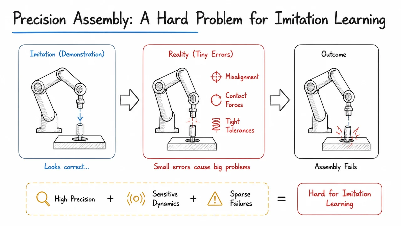
Imagine teaching a robot to plug a delicate connector into a port with sub‑millimeter clearance. The task demands precision, yet the robot learns from human demonstrations: someone teleoperating the arm, guiding it slowly to the target. Humans naturally correct micro‑misalignments using visual feedback, but the robot sees only a stream of joint positions and gripper commands. The naive approach—record the demo trajectories and train a policy to reproduce them—is behavior cloning (BC). For standard pick‑and‑place tasks, recent advances like action‑chunking transformers have made BC remarkably effective. However, high‑precision assembly exposes a set of stubborn failure modes. This section unpacks why such tasks remain a hard problem for imitation learning, setting the stage for a refinement strategy that goes beyond cloning.
The central tension lies in the nature of the imitation data. Demonstrations provide expert trajectories, but they are on‑policy samples from the human’s own policy, not the robot’s. When a BC policy deviates even slightly from a demonstrated state—perhaps because the gripper is a millimeter off, or the peg encounters unexpected friction—it enters states that the training distribution never covered. The learned mapping from observation to action becomes unreliable, and the error compounds. In high‑precision assembly, tolerance is essentially zero: a miniscule orientation error turns a successful insertion into a failed jam. The policy, trained to minimize error on the training set, has no incentive to recover from such deviations because it never saw them during training. This is the distribution shift problem, and in tight‑clearance tasks it is catastrophic.
Action chunking, which predicts a sequence of future actions at once, amplifies the difficulty. Chunking improves smoothness and reduces the effective horizon during training, but at deployment it introduces open‑loop execution within each chunk. The robot commits to, say, actions before reassessing the state. If the initial state already contains a small error, executing the whole chunk blind can drive the end‑effector far off course. In assembly, a single chunk that prescribes a straight‑line approach might collide with the chamfered edge of the hole; a closed‑loop controller would detect the contact force and adjust, but the chunked BC policy naively continues pushing. This open‑loop drift is a primary cause of performance saturation: beyond a certain dataset size or model capacity, BC’s success rate plateaus well below 100% because no amount of data can cover every possible off‑track scenario.
Mathematically, we can view the chunked policy as producing a trajectory conditioned on the current observation . The ground‑truth expert action sequence would bring the robot to the intended next state, but the learned is an imperfect approximation. The rollout error after steps depends on the dynamics : . Even if the average per‑step action error is small, the accumulated state deviation can grow super‑linearly, especially when the dynamics involve contact that abruptly changes the system’s response. The standard BC objective treats each step equally, ignoring the cascading nature of errors. In precision tasks, this ignores the fact that a 1‑degree orientation error at the start of insertion causes a completely different contact interaction than a perfect alignment—yet the squared loss penalizes them identically during training.
Why not simply collect more data? Extra demonstrations cover more variations, but they are still near‑optimal. They rarely include recovery behaviors—dropping the peg, retrying, wiggling—because the human demonstrator rarely makes mistakes. The distribution of states in the dataset remains concentrated around successful trajectories. The policy never learns to handle the fringe states it will inevitably visit due to its own imperfections. This is the infamous “covariate shift” cycle: imprecision → distribution shift → larger error → further shift. Scaling up data collection eventually hits diminishing returns, and for many real‑world assembly tasks, the cost of thousands of demonstrations becomes prohibitive anyway.
A final, subtle layer of difficulty comes from the sensing gap. Human demonstrators rely on vision and haptics that are richer than the robot’s available sensors. A policy trained solely on wrist‑mounted camera images or joint states must infer alignment from impoverished signals. Even a perfectly cloned trajectory can fail if the downstream vision system introduces latency or noise that the demonstrator never encountered. The combination of distribution shift, open‑loop chunk commitment, and sensor mismatch creates a barrier that pure imitation learning, even with modern architectures, struggles to cross.
The visual below captures this predicament succinctly. A robotic gripper is shown attempting to insert a narrow peg into a hole, with a clear millimeter‑scale gap indicating misalignment. Arrows and handwritten‑style labels highlight how distribution shift drives the policy into unseen states, how open‑loop action chunks ignore that error for the chunk duration, and how the accumulated deviation leads to a hard contact or jam. The diagram serves as a touchstone for the central claim: high‑precision assembly is not just a harder version of pick‑and‑place—it is a qualitatively different challenge where small errors cascade into unrecoverable failures. Recognizing this motivates the need for a refinement process that can actively correct such errors, a process we will develop in the coming sections.
Given the steep demands of precision assembly—sub‑millimeter clearances, brittle parts, and the need for reactive fine‑motion strategies—it is natural to wonder whether simply increasing the volume of expert demonstrations could lift an imitation‑learned policy to expert reliability. After all, scaling data has repeatedly proven to be a powerful lever in computer vision and natural language processing, and behaviour cloning (BC) would, in principle, converge to the optimal policy as the dataset covers the entire state‑space under the expert distribution.
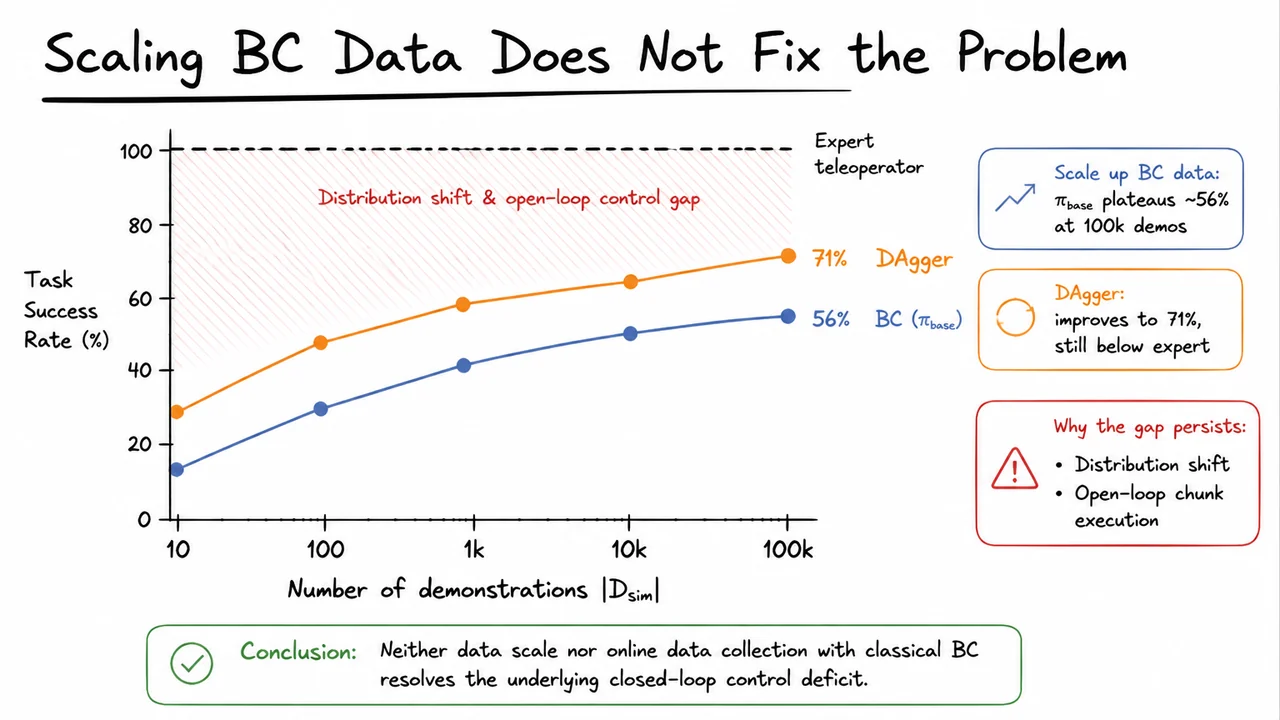
Alas, in tasks like the round_table assembly benchmark, the data‑scale narrative breaks down. Even when the simulator pumps out expert trajectories, the trained base policy plateaus at a modest ~56% success rate. A classic BC with an action‑chunking architecture never crosses the threshold needed for practical deployment, no matter how many demonstrations are added. This saturation is not a quirk of a particular training run; it is a systematic ceiling imposed by the interplay between distribution shift and open‑loop chunk execution.
The root cause is that offline demonstrations are collected under a closed‑loop expert—a teleoperator who continuously observes the environment and adjusts each motion in real time. The resulting dataset therefore contains state–action pairs from a narrow, expert-induced manifold. During execution, however, the policy’s predicted action chunk is applied for several time steps without any environmental feedback. Even tiny, physically imperceptible tracking errors accumulate over the chunk horizon. Because those perturbed states were never visited in the training data, the policy increasingly drifts off the expert manifold. The open‑loop block then commits to a rigid sequence of actions, making it impossible to react to the new visual or force‑torque readings that appear partway through the chunk. The policy lacks the closed‑loop reactivity that the original expert used to correct such deviations—it cannot, for example, sense a gradual misalignment and nudge the peg back into insertion.
This issue persists even when we move beyond purely offline BC and incorporate online expert queries via DAgger. DAgger interleaves policy rollouts with expert corrections: whenever the policy’s performance deviates, the expert provides corrective labels at the visited states, and those labelled states are added to the dataset. On the round_table task, DAgger lifts the success rate to 71% at the largest dataset size—a meaningful improvement, yet still far below the expert’s near‑perfect rate. Why does the gap remain? Because DAgger still treats the policy as a static open‑loop chunk generator. The additional states fed back by the expert do help the policy learn to handle some common failure modes, but the policy itself remains structurally blind to per‑timestep sensory feedback when deployed. The open‑loop chunk execution step length is fixed, so the policy cannot engage in the continuous micro‑adjustments that a human teleoperator performs dozens of times per second. In other words, even an online expert cannot teach a chunked model to be closed‑loop, because the model’s action interface fundamentally precludes that kind of control.
The combined effect is a persistent control deficit that no amount of offline or online demonstration data can fill. The policy’s action‑prediction horizon is a coarse, ballistic sketch of a motion plan, not the reactive, feedback‑driven sequence that precision tasks require. This insight tells us that the problem is not one of insufficient supervision but rather one of policy structure: the model must be capable of issuing corrections on every single control step, informed by the latest sensor measurements, to match the expert’s real‑time dexterity. That capability will require a new training paradigm—one that later sections will frame as residual reinforcement learning—but before moving there, it is helpful to see the empirical evidence in compact form.
The figure below plots the success rate against the number of demonstrations (log‑scale) for both (BC) and DAgger, with the expert teleoperator baseline at 100%. The blue BC curve climbs early but flattens around 56%, while the orange DAgger curve progresses further, ending at 71%. The shaded region between DAgger and the expert line is annotated as the “distribution shift & open‑loop control gap.” This visual consolidates the message: scaling data does not resolve assembly failures, because the underlying closed‑loop control deficit is a structural limitation that deeper data pipelines alone cannot address. The persistent gap remains the motivating force behind the shift from imitation to refinement.
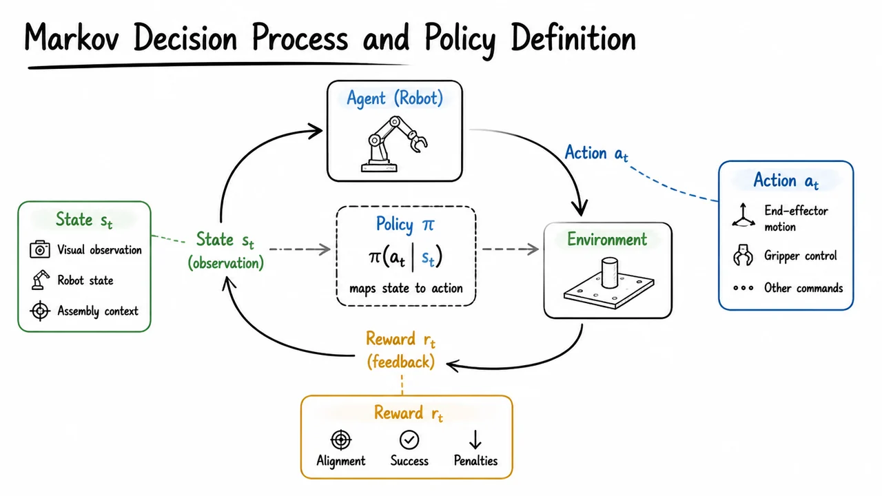
The failure of pure behavior cloning to scale into high‑precision regimes, which we explored in the previous section, makes it clear that supervised imitation alone cannot solve the assembly problem. To understand why and how we can fix it, we need a formal language for the robot’s interaction with the world. That language is the Markov Decision Process (MDP), a framework that models every task as a sequential feedback loop. Only by grounding our policies in this loop can we expose the brittle open‑loop assumption behind action chunking and design a correction mechanism that respects the true dynamics of the task.
An MDP is a tuple . The state describes the world at time : for a robot arm inserting a peg, this could be joint angles, end‑effector pose, forces, and camera images. In practice we rarely see the perfect state; we work with an observation that contains the robot’s proprioception and one or more RGB images. The action is the command we send to the robot – typically a small delta in the 6‑DoF end‑effector pose. The dynamics capture the physics of the robot and the environment, a stochastic transition that can include friction, compliance, and sensor noise. After each transition the agent receives a reward , a scalar that encodes how well the step moved the task forward (e.g., insertion depth, alignment error, final success flag), and the discount factor weights immediate versus future rewards. A trajectory is the sequence generated by repeatedly applying a policy and sampling from the dynamics.
A policy is the agent’s brain: it maps observations to actions. It can be deterministic, , or stochastic, . The objective in reinforcement learning is to find a policy that maximizes the expected cumulative discounted reward . Imitation learning, by contrast, abandons the reward and instead tries to mimic an expert’s actions given the same states. Behavior cloning treats the problem as supervised regression: given a dataset of expert observation‑action pairs , we fit a policy that minimizes (or a likelihood loss for a diffusion policy). This is fast and stable, but it never sees the consequences of its own actions – it ignores the feedback loop altogether.
In robotic assembly, the dominant BC paradigm is action chunking: the policy, conditioned on a single observation , produces a contiguous block of future actions that will be executed open‑loop until the next observation. Formally, we can treat this chunk as a single macro‑action, but once it is issued the robot blindly follows it for steps, accumulating any errors without correction. The MDP perspective makes the flaw crystal clear: the learned mapping was trained on expert trajectories where state transitions followed the expert’s distribution, but at test time small deviations in the early actions of a chunk push the state into unfamiliar territory. The very next observation comes from a different distribution, so the policy’s next chunk may be even worse. This is distribution shift, amplified by the open‑loop nature of the chunk. In tasks demanding sub‑millimeter precision – like electrical connector insertion – the resulting drift quickly racks up failures, no matter how many extra demonstrations we collect.
To break this vicious cycle we need to reintroduce closed‑loop feedback at every time step, while still capitalizing on the strong behavioral prior of a well‑trained BC policy. The residual policy framework does exactly that. We freeze a chunked BC policy as a base policy and then train a lightweight residual policy that outputs a per‑timestep additive correction to the nominal action. At each step, the actual action sent to the robot is where is the index within the current chunk. The correction is computed from the current observation (and possibly a short history) using a small network or even a linear model. Because the base policy handles the coarse movement, the residual policy only has to learn local adjustments that keep the trajectory on the narrow expert manifold. Crucially, the whole system now observes the state at every step and can correct for any drift before it compounds. The MDP view shows us that we are effectively transforming an open‑loop chunked policy into a reactive, closed‑loop policy that respects the temporal structure of the decision problem.
The visual below encapsulates this progression. It depicts the classic MDP cycle – state, action, reward, next state – and labels the agent’s internal composition: a frozen base policy that provides a chunk of nominal actions, and a residual network that injects per‑step corrections. This diagram makes the flow of time and feedback explicit, preparing us to formally define the base diffusion policy in the next section and then the residual RL objective that turns a brittle imitator into a robust assembler.
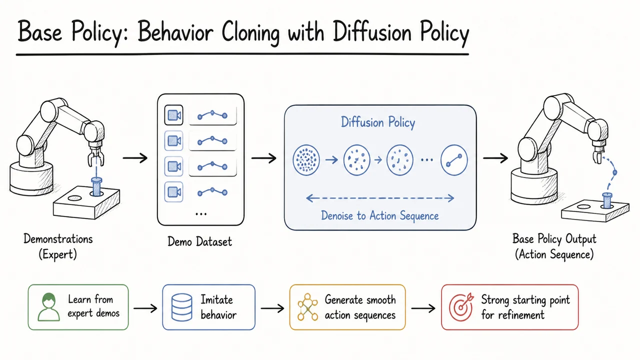
To design a controller that can perform sub-millimeter insertion tasks, the first natural step is to learn from demonstration. We assume access to a dataset of expert trajectories, each consisting of high‑frequency observations paired with precise actions. The most straightforward way to turn this data into a policy is behavior cloning (BC): treat the decision‑making problem as supervised regression from observation to action, and train a model to mimic the expert’s conditional distribution. Early attempts used simple feed‑forward architectures or recurrent networks, but in high‑precision robotic assembly, these struggled to capture the multi‑modal, long‑horizon nature of the required behavior. An expert might, for instance, approach a tight peg‑in‑hole task from slightly different angles or adapt a compliant insertion strategy based on sub‑millimeter force feedback—the action distribution at a given state is often complex and far from a single mode. This is where diffusion models enter as the backbone of our base policy.
A diffusion policy formulates the problem as learning a generative model of the action chunk—a contiguous block of future actions—conditioned on the current observation. The key idea is to start from pure random noise and, over a sequence of denoising steps, arrive at a clean action chunk that matches the expert distribution. During training, we take expert action chunks, gradually corrupt them with Gaussian noise according to a predefined forward noising schedule (usually a variance‑preserving SDE or DDPM‑style discrete steps), and train a score network to predict the noise added. The observation could be a single image, a short history of images, or proprioceptive readings. By conditioning the denoising process on , the model learns the conditional score function , effectively capturing the full multi‑modal action distribution.
At inference time, we sample an initial action chunk from isotropic Gaussian noise and then repeatedly apply the learned reverse process: where is fresh noise, and the steps contract the distribution toward the learned conditional data manifold. After typically 50–100 denoising iterations, we obtain a plausible action chunk of length , e.g., 16 actions stretching over the next 0.5 seconds. Because the generative process is stochastic, the policy naturally produces diverse actions when the expert distribution itself is broad, and smoothly converges to a sharp mode when the correct action is unambiguous.
The practice of outputting an action chunk rather than a single action is central to the policy’s effectiveness. By predicting a sequence of actions and executing them in an open‑loop fashion for steps (or until the next re‑planning cycle if using receding‑horizon control), the policy mitigates issues like intermittent sensor dropouts and induces temporal consistency. Without such a horizon, a per‑timestep BC policy would easily drift into states where it has never seen expert corrections, leading to compounding errors—the classic distribution shift problem. The chunked diffusion policy, in contrast, can plan a short trajectory that respects the dynamics of the task, even if the exact state trajectory deviates slightly from those seen in training.
Still, at its core, this remains a purely open‑loop behavior cloning method: once the chunk is generated, the actions are played out without further recourse to the environment’s feedback until the next re‑planning step. In a high‑precision assembly setting, positional errors on the order of a millimeter can cause the robot to jam, miss the hole entirely, or exert dangerous forces. The base policy may achieve near‑perfect success in the training distribution—when the environment and initial conditions closely match the demonstrations—but its performance saturates and sharply degrades under distribution shift. This saturation motivates the need for closed‑loop corrections that we formalize later as residual RL.
The visual below summarises the diffusion policy pipeline. It shows the flow from observation encoding through the iterative denoising process: starting from a cloud of random noise, conditioned on the visual and proprioceptive input, the model refines a candidate action chunk over several denoising steps until a clean, executable sequence emerges. The diagram also emphasises the action‑chunk horizon and the open‑loop execution phase, reinforcing the compactness of the design: a frozen diffusion model that acts as a strong but imperfect base. Understanding this architecture is essential before we dissect its failure modes and introduce the residual correction strategy that turns imitation into refinement.
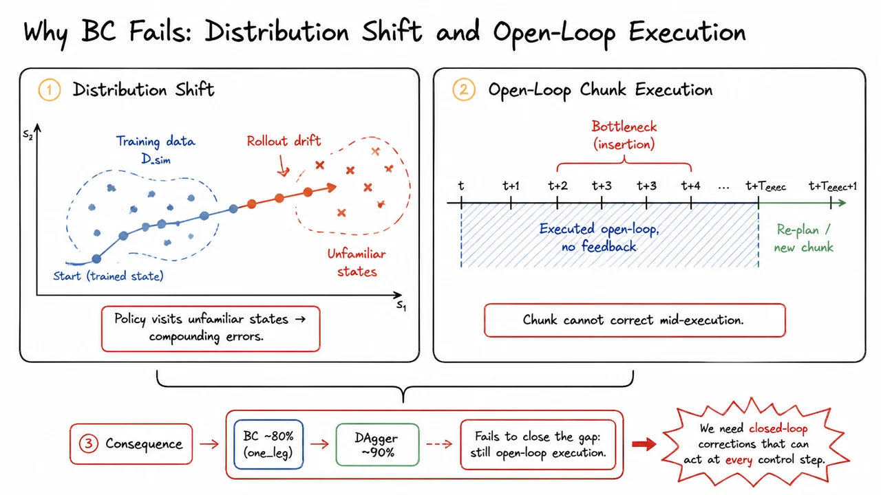
After constructing a base diffusion policy via behavior cloning on expert demonstrations, a natural expectation is that performance will scale with more data, a better architecture, or even iterative correction techniques like DAgger. Yet, on high‑precision assembly benchmarks such as the NIST one_leg insertion, BC‑based policies consistently saturate well below full task completion — often around 80 % for the original BC and no higher than ~90 % even with DAgger’s on‑policy corrections. The stubborn ceiling reveals that the remaining ~10 % of trials fail for deeply structural reasons, not simply because the training set is incomplete or the imitation objective is imperfect. Two intertwined culprits lie at the heart of this failure: distribution shift and open‑loop chunk execution. Understanding each one in detail is the key to motivating a fundamentally different class of solutions that introduce closed‑loop, per‑timestep corrections.
The BC objective minimises the expected negative log‑likelihood under the demonstration distribution: During training, the policy sees states drawn exclusively from the expert’s trajectories, which are collected inside a controlled simulator or a carefully reset environment. At deployment, however, the same policy generates its own trajectory; the distribution of visited states diverges from the training distribution as small prediction errors push the robot into regions of the state space it has never practised recovering from. This is the classic covariate shift problem: each mistake makes the next state slightly different, and because the policy was never trained on that perturbed state, it produces an even noisier action, compounding the drift. The process is insidious — what begins as a sub‑millimetre offset in a connector approach can cascade into a completely missed insertion attempt after a few timesteps.
DAgger partially mitigates this drift by periodically rolling out the current policy, asking a human or a privileged expert to relabel the visited states, and then retraining on the aggregated dataset. This explicitly forces the policy to see states from its own induced distribution, thereby reducing the gap between training and deployment distributions. Empirically, DAgger lifts success rates from ~80 % to ~90 % on one_leg, confirming that distribution shift is a real bottleneck. Yet the remaining gap persists because DAgger cannot correct errors that explode inside an action chunk — a failure mode that distribution shift alone does not capture.
The second culprit, open‑loop chunk execution, is a direct consequence of how diffusion‑based policies typically operate. The base policy outputs an action chunk of length : and the robot executes the first actions (usually a subset, e.g., ) before re‑planning. In practical systems, ranges from 4 to 16 steps, spanning roughly 100–400 ms. During that window, the policy is completely blind to new observations; it acts as an open‑loop plan that cannot absorb real‑time feedback. If a critical bottleneck state — say, the precise moment of peg‑hole alignment just before insertion — falls entirely inside the executed portion of a chunk, the robot must commit to a sequence of pre‑computed actions generated from an earlier, potentially stale observation. Any small misalignment at the chunk’s start is then “baked in” and executed faithfully, with no chance to correct until the chunk ends and a new observation triggers a fresh plan.
The interplay of these two failures is what makes high‑precision tasks so brittle. When a policy under distribution shift produces a slightly inaccurate action at the start of a chunk, the downstream actions in that same chunk are based on an already‑inaccurate state trajectory — they cannot adjust. Even if the policy were perfect on the training distribution, the unavoidable, minute discrepancies at deployment (due to sensor noise, hardware backlash, or minute pose errors) create a gap that the open‑loop execution amplifies. Thus, DAgger’s on‑policy relabeling helps the policy predict better actions from a single observation, but it does not give the policy the ability to react mid‑chunk. The compounding of errors within a chunk effectively makes the effective horizon of open‑loop planning longer than the system’s real‑world stability, especially for insertion tasks that require fine mechanical accommodation at precisely the right instant.
The visual that accompanies this section distils these two failure modes into a clear, side‑by‑side comparison. On the left, a 2‑D state‑space sketch shows a dense cluster of training points from and a drifting trajectory that veers away from those familiar states, with arrows marking the compounding errors. The caption underscores that the policy visits unfamiliar states, and DAgger can only partially pull it back. On the right, a timeline of discrete control ticks highlights a chunk execution window, shading the bottleneck insertion step and labelling the entire span as “executed open‑loop, no feedback.” The dashed line at chunk termination reminds us that re‑planning occurs only once every steps. Together these panels make the argument tactile: without closed‑loop corrections that can interleave every single control step, the system remains vulnerable to both long‑term drift and short‑term blindness. This diagnosis sets the stage for the residual RL framework, which preserves the chunked planner’s foresight but augments it with a reactive corrector that can act at every timestep, no matter where a bottleneck falls.
We’ve seen that behavior cloning with action chunks fails when open‑loop execution encounters bottleneck states. Chunked policies treat the future as a fixed plan, oblivious to deviations that accumulate after the first timestep. The core difficulty is not that the demonstrations lack information—they are rich—but that the planner is forced to commit to a rigid sequence without the benefit of intermediate state feedback. This rigidity leads to compounding errors: a slight misalignment in an insertion task, for example, cannot be corrected until the next chunk is recomputed, by which time the part may have jammed or deflected.
The fundamental insight is to stop forcing the entire policy to be either reactive or open‑loop. Instead, we can decompose control into two cooperating components that operate at different timescales. A coarse temporal planner can still generate a macro‑level trajectory, perhaps learned from demonstrations, while a fast reactive corrector intervenes at every control step to compensate for local errors and uncertainty. This decomposition mirrors how many engineered systems work: a global plan provides guidance, and a local feedback controller handles high‑bandwidth disturbances. The challenge for learning is to realize such a decomposition without compromising the skill encoded in the original demonstrations and without discarding the planner’s global knowledge.
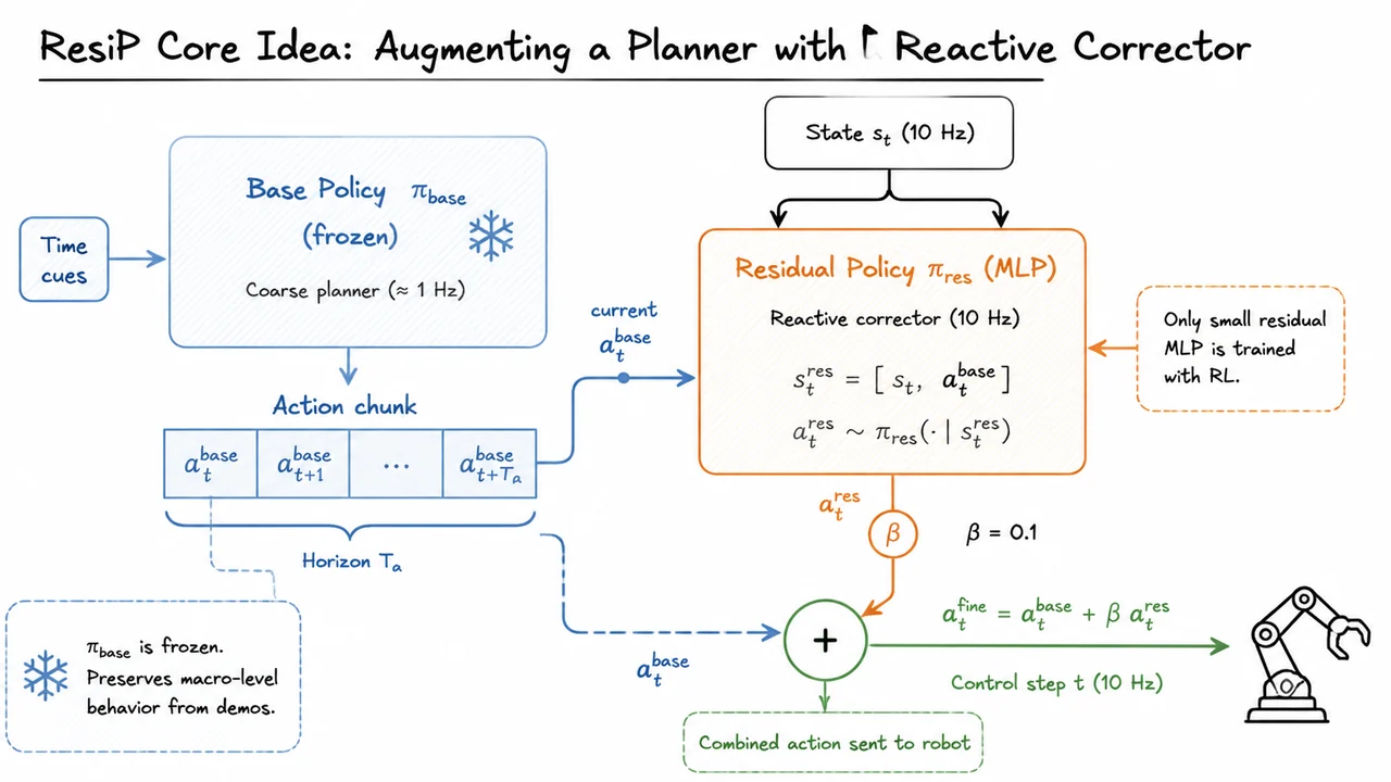
ResiP, short for Residual Policy, answers this challenge by keeping the base BC policy frozen and training only a lightweight residual network with reinforcement learning. The base policy remains exactly as it was trained from demonstrations; it outputs entire action chunks at a low effective frequency—roughly 1 Hz—representing a coarse temporal plan for the next several seconds. The residual corrector runs in parallel at the full control frequency (10 Hz), observing the true state of the robot and environment together with the planned base action for that timestep. Its job is to produce a small corrective shift.
The interaction between planner and corrector is cleanly formalized through an augmented state. At each control step , the residual policy observes an enhanced input vector
where is the base action prescribed by the chunk for the current timestep. This couples the corrector to the planner’s intent: it knows what the base policy would do, but can modify it based on the actual sensor feedback. The residual action is sampled from a stochastic Gaussian policy
and the final action sent to the robot is a simple additive combination
The scalar acts as a bounded gain, ensuring that corrections remain modest relative to the base plan. This design intentionally limits the residual policy’s authority: it can adjust, but not override, the demonstrated macro‑behavior.
Because only the residual policy is trained with RL, the planner’s demonstration‑level quality is never forgotten. No catastrophic forgetting occurs; in fact, the base policy provides a strong behavioral prior that dramatically reduces exploration. The residual network, typically a small multi‑layer perceptron, learns to produce per‑timestep closed‑loop corrections that push the system toward success regions that dense reward signals can recognize. For instance, in a peg‑insertion task, a purely open‑loop chunk may miss the hole if the gripper’s approach is slightly misaligned; the corrector, seeing the visual or force feedback, can nudge the end‑effector just enough to align and seat the peg—without ever relearning the overall insertion strategy.
This separation of roles solves the distribution‑shift problem at its root. The base policy never sees out‑of‑distribution states because it never receives online feedback; it merely replays its pre‑computed plan. The residual policy, on the other hand, is trained entirely online with domain randomization and reward shaping, so it learns to handle the kinds of errors that arise in practice. The combined system gracefully merges the temporal abstraction of a planner with the reactive precision of a feedback corrector.
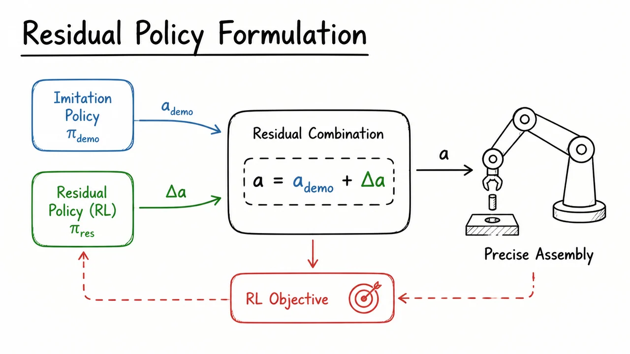
The structural elegance of ResiP becomes clear when we diagram the two cooperating modules side by side. The frozen base policy sits on one side, outputting a chunk of base actions that extend into the future. At each control step, the relevant planned action is fed forward alongside the current state into the residual corrector—a compact MLP—which produces a small adjustment. Their sum, scaled by , becomes the fine command sent to the robot. The diagram visualizes this as a time‑unrolled pipeline: a solid arrow from the state sensor entering the residual module, a dashed arrow carrying the planned action into the same module, and the two combining at a summation node labeled . Only the residual pathway is active during RL, marked by a distinct color to emphasize that the planner is frozen, preserving the macro‑skill while the corrector injects the feedback intelligence needed for high‑precision assembly.
The idea of augmenting a planner with a reactive corrector is deceptively simple, but turning it into a precise algorithmic component demands a clean formal separation between what is planned and what is corrected online. The residual policy formulation provides exactly that. It does not ask us to retrain the base policy, nor to tune a monolithic network that balances imitation and reinforcement. Instead, it composes two functions that each have a clear, limited responsibility, and it trains only the corrective part, leaving the planner frozen. This additive decomposition is the backbone of ResiP and is what enables the system to achieve sub‑millimeter assembly success rates without destroying the behavioral priors learned from demonstrations.
Let the base policy be a frozen behavior‑cloning model, denoted , that predicts action chunks. At any decision instant it emits a sequence of future actions , where is the chunk horizon and is the observation. When executing this chunk open‑loop, the robot would simply follow without further sensory feedback. That is the core fragility: a small tracking error at the first step can cause the entire remainder of the chunk to be executed in a slightly shifted world state, and the open‑loop plan has no mechanism to recover. The residual policy, , is introduced at every control timestep to correct this drift. Even while a chunk is being executed, at each step the robot receives a new observation and computes a correction . The final action sent to the robot is therefore:
The correction can be interpreted as a learned additive bias that shifts the base action just enough to nudge the end‑effector back toward a successful trajectory. Critically, the residual policy can condition on the base action; this allows it to understand what the open‑loop plan intended and avoid working against it. In many implementations, also receives a short history of past observations, enabling it to model transient dynamics without burdening the base planner with additional temporal context.
This formulation draws a sharp line between global task structure and local feedback control. The frozen BC policy retains the large‑scale motion pattern—the high‑level sequence of grasp, approach, insert, rotate—while the residual policy handles the micro‑adjustments that real‑world geometry and friction demand. Because is not updated during reinforcement learning, the system never suffers catastrophic forgetting of the demonstrated motion plans. The residual component is initialized near zero (e.g., as a network with small outputs) so that early interactions still behave like the BC policy, and then it gradually learns to add only the necessary corrections. This is a far gentler and more sample‑efficient starting point than training a diffusion policy from scratch with RL or even jointly fine‑tuning the entire stack.
Compare this with a direct RL fine‑tuning approach. If we allowed the chunked BC policy’s parameters to be updated, the optimizer might rapidly overwrite the imitation prior to chase short‑term reward, especially when reward signals are sparse and noisy. Keeping frozen creates an anchor in action space, and the residual RL problem becomes a kind of perturbation learning around a strong baseline. Moreover, because the residual policy operates at the full control frequency (each timestep), it acts as a closed‑loop stabilizer that can compensate for the open‑loop deficiencies of chunk execution. Even if the BC policy replans a new chunk at every steps, the residual corrections apply inside each chunk, effectively turning a discrete replanning process into a continuous closed‑loop controller.
The accompanying diagram distills this architecture into an easily readable schematic. It shows the frozen chunked BC policy block producing a base action stream, and a parallel residual policy block—also receiving the current observation—outputting a correction that is summed into the final motor command. The visual emphasizes the additive composition, the freeze on the BC weights, and the closed‑loop aspect by drawing a feedback arrow from the observation to the corrector. A clean sketch of temporal flow (chunk horizon vs. per‑timestep correction) reminds the viewer that the base plan is coarse‑grained while the residual is fine‑grained. This separation of concerns, captured in a glance, is the conceptual key to understanding why ResiP can achieve both robustness and precision.
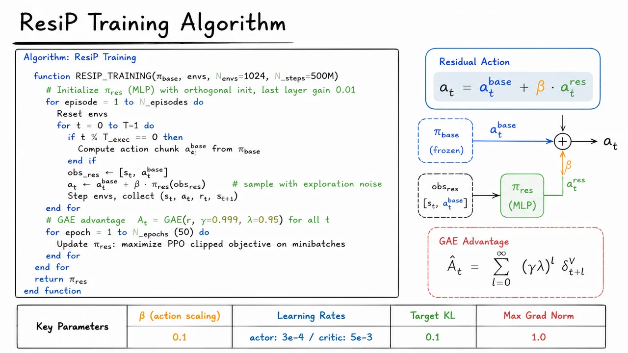
With the residual action decomposition in place, the next challenge is designing a training routine that reliably discovers the small, high-precision corrections without destabilizing the already competent imitated behavior. Directly fine‑tuning the entire policy via reinforcement learning would risk forgetting the delicate alignment learned by behavior cloning on high‑precision tasks—exactly the failure mode we set out to avoid. ResiP addresses this with a carefully orchestrated loop that keeps the base policy frozen, uses massive parallelism to gather diverse correction experiences, and applies trust‑region policy optimization on a lightweight residual network.
At the heart of ResiP training lies the interplay between open‑loop action chunks from the frozen base policy and per‑timestep closed‑loop corrections. The base policy , often a diffusion or autoregressive model trained via behavior cloning, generates action chunks every timesteps. These chunks are sequences of future base actions intended to be executed open‑loop. Between chunk computations, the environment evolves and discrepancies accumulate. The residual policy is invoked at every single timestep: it receives a composite observation consisting of the current state and the pre‑computed base action for that step, , and outputs a correction scaled by . The actual action sent to the robot is . This design fuses the long‑horizon predictability of chunked imitation with the instantaneous reactivity of residual RL.
The training loop itself is an on‑policy reinforcement learning cycle built for stability at scale. It initializes as a small multi‑layer perceptron with orthogonal weight initialization and a last‑layer gain of just . That choice makes the residual output nearly zero at the outset, so the initial policy behaves almost identically to the frozen base—an important precondition for safe exploration. During each episode, parallel environments are stepped forward synchronously. Whenever is a multiple of , the base policy is queried to produce a fresh chunk of base actions; otherwise the previously computed chunk continues to supply . The residual policy samples its correction with additional exploration noise, and the combined action is executed, collecting rewards and next states.
Once a full batch of timesteps has been gathered across all environments, ResiP computes Generalized Advantage Estimation (GAE), a standard technique that balances bias and variance in the advantage estimate:
With and , the advantage spans long horizons and captures the cumulative consequences of small assembly‑stage deviations. A high discount factor is essential in precision tasks where success is determined only at the final step; dropping would wash out the signal needed to learn sub‑millimeter corrections. The value function is a separate critic network trained jointly with the residual actor.
Following GAE, the residual policy is updated for epochs over the collected rollout data using the PPO clipped surrogate objective. Each epoch minibatches the experiences, normalizes advantages, and optimizes the policy while penalizing deviations from the previous behavior distribution. A target KL divergence of and a maximum gradient norm of prevent overly large updates that could destroy the fragile residual corrections. Notably, the actor learning rate () is kept lower than the critic learning rate (), allowing the value function to quickly adapt to the reward landscape while the policy moves more cautiously. After the epochs, the loop resets the environments and repeats, for a total budget of roughly 500 million environment steps.
This interleaved design yields several practical advantages. Because the base policy is never updated, the strong behavioral prior from imitation is permanently preserved; the residual RL only has to model the difference between the open‑loop plan and what the task truly demands. The massive parallelism ( envs) provides a rich variety of perturbation contexts, which is crucial for learning corrections that generalise across subtle geometric variations. And the trust‑region updates guarantee that the residual corrections remain small even as performance climbs, avoiding the catastrophic overwriting that plagues direct fine‑tuning of diffusion or chunked policies.
The visual below brings these algorithmic pieces together in a clean pseudocode arrangement. It highlights the periodic base‑chunk computation, the per‑step composition with the scaled residual, and the two‑phase structure of data collection followed by multi‑epoch PPO optimization. A small parameter table at the bottom lists the key scaling factor, learning rates, KL target, and gradient clipping threshold—the numerical settings that make the whole loop work in practice. Seeing the training procedure as a single coherent block helps anchor the intuition that ResiP is at its core a lightweight, massively parallel reinforcement learning shell wrapped around a frozen imitation core, a recipe that turns out to be remarkably effective for high‑precision robotic assembly.
The previous section detailed how ResiP freezes the base policy and learns a compact residual MLP that adds a per‑timestep correction within a tightly bounded neighborhood. A natural question arises: why not simply unfreeze the base policy and fine‑tune it directly with reinforcement learning? After all, that seems like the most obvious path — take the imitation‑trained network, initialize the RL policy with its weights, and apply a standard on‑policy algorithm such as PPO. The reality, especially for high‑precision contact‑rich tasks, is far less forgiving. Direct RL fine‑tuning of chunked or likelihood‑free policies suffers from two principal failure modes, both rooted in the unique structure of behavior‑cloned action chunking and the mathematical limitations of modern deep RL.
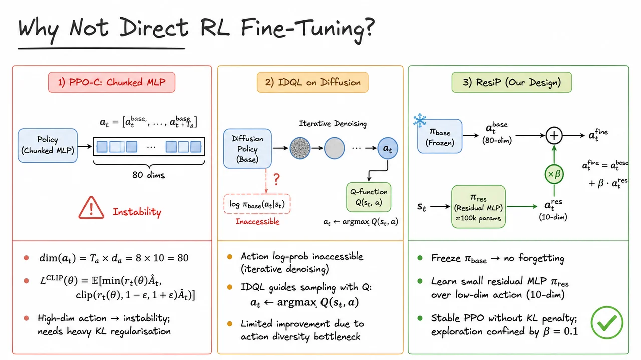
Consider first the approach of applying PPO to the chunked MLP policy — call this PPO‑C. The base policy predicts an entire action chunk
where and each action vector has dimensions. PPO’s clipped surrogate loss,
is designed to tame policy updates via a trust‑region‑like clipping mechanism. However, the raw dimensionality of the policy’s output space introduces enormous variance into the policy gradient estimator. Even with clipping, the advantage estimates become noisy when a single scalar reward signal must guide an 80‑dimensional multivariate Gaussian. Consequently, the optimizer demands heavy KL regularisation to prevent the policy from collapsing to a degenerate distribution or drifting far from the imitation prior, but that very regularisation stifles meaningful improvement, leaving final performance stuck near the behavior‑cloned baseline. Training instability, forgetting of delicate assembly primitives, and the need for impractically large batch sizes are the rule, not the exception.
The second candidate is fine‑tuning a diffusion policy via Q‑guided sampling, a strategy often instantiated as IDQL (Implicit Diffusion Q‑Learning). Diffusion models do not expose an explicit action log‑probability — the iterative denoising process makes intractable. Consequently, one cannot plug the policy into any likelihood‑based RL objective (PPO, AWR, etc.). Instead, IDQL trains a separate action‑value function and, at inference time, biases the denoised action sample towards higher Q‑values:
But here the frozen base model’s limited action diversity becomes a hard bottleneck. The Q‑function is only trained on the actions produced by the base policy’s distribution; it cannot reliably evaluate actions far from that support. Moreover, the diffusion model itself remains frozen to prevent forgetting, so its denoising process can only explore a narrow corridor around the original BC actions. The result is that IDQL achieves little more than a local re‑ranking of already‑familiar behaviors, rarely discovering the precise, closed‑loop corrections that high‑accuracy assembly demands. In short, both PPO‑C and IDQL hit a performance ceiling that imitation alone cannot breach.
ResiP circumvents these obstacles by a simple but powerful design decision: freeze the base policy completely and introduce a separate, lean residual policy that outputs a low‑dimensional per‑timestep correction
with . This factorization decouples the RL problem from the high‑dimensional chunked space: PPO now only needs to learn a small residual MLP (roughly 100k parameters) on a 10‑dimensional action, yielding low‑variance gradient estimates and stable training without any KL penalty. The exploration is confined by the small , naturally constraining the policy to remain near the well‑behaved BC prior and virtually eliminating catastrophic forgetting. Furthermore, because the base policy is a feed‑forward MLP (or a diffusion decoder) that is frozen, ResiP is indifferent to whether the base policy offers a tractable log‑prob — it sidesteps the intractability problem entirely.
The visual comparison below brings these contrasts into sharp relief. On the left, PPO‑C is depicted as a box gushing an 80‑dimensional vector, annotated with a warning symbol for high‑dimensional instability and the PPO surrogate loss equation; it shouts heavy KL regularisation, training collapse. In the center, IDQL on Diffusion shows the iterative denoising process with a Q‑function that can only influence sampling indirectly, the log‑prob marked with a question mark to indicate its inaccessibility, and the note “limited action diversity” underneath. On the right, highlighted in green with a checkmark, ResiP (Ours) exhibits a frozen base chunk policy feeding into a tiny residual MLP; the scalar gate and the residual addition are drawn prominently, with the label “stable PPO, no KL penalty, bounded exploration.” The diagram thus serves as a compact summary of the three architectural choices, making it immediately clear why ResiP’s structured decomposition is the key to bridging imitation and reinforcement in high‑stakes robotic assembly.
Our earlier exploration showed why applying online reinforcement learning directly to a chunked diffusion policy is fraught: the loss of per‑timestep feedback, the open‑loop nature of chunked execution, and the covariate shift when small errors accumulate over a horizon. Before we can properly judge whether a residual correction can salvage the situation, we need a rigorous testing ground and a carefully selected set of baselines. The goal is to isolate the effect of closed‑loop refinement while keeping everything else — the base policy architecture, the training data, and the evaluation protocol — exactly the same across all contenders.
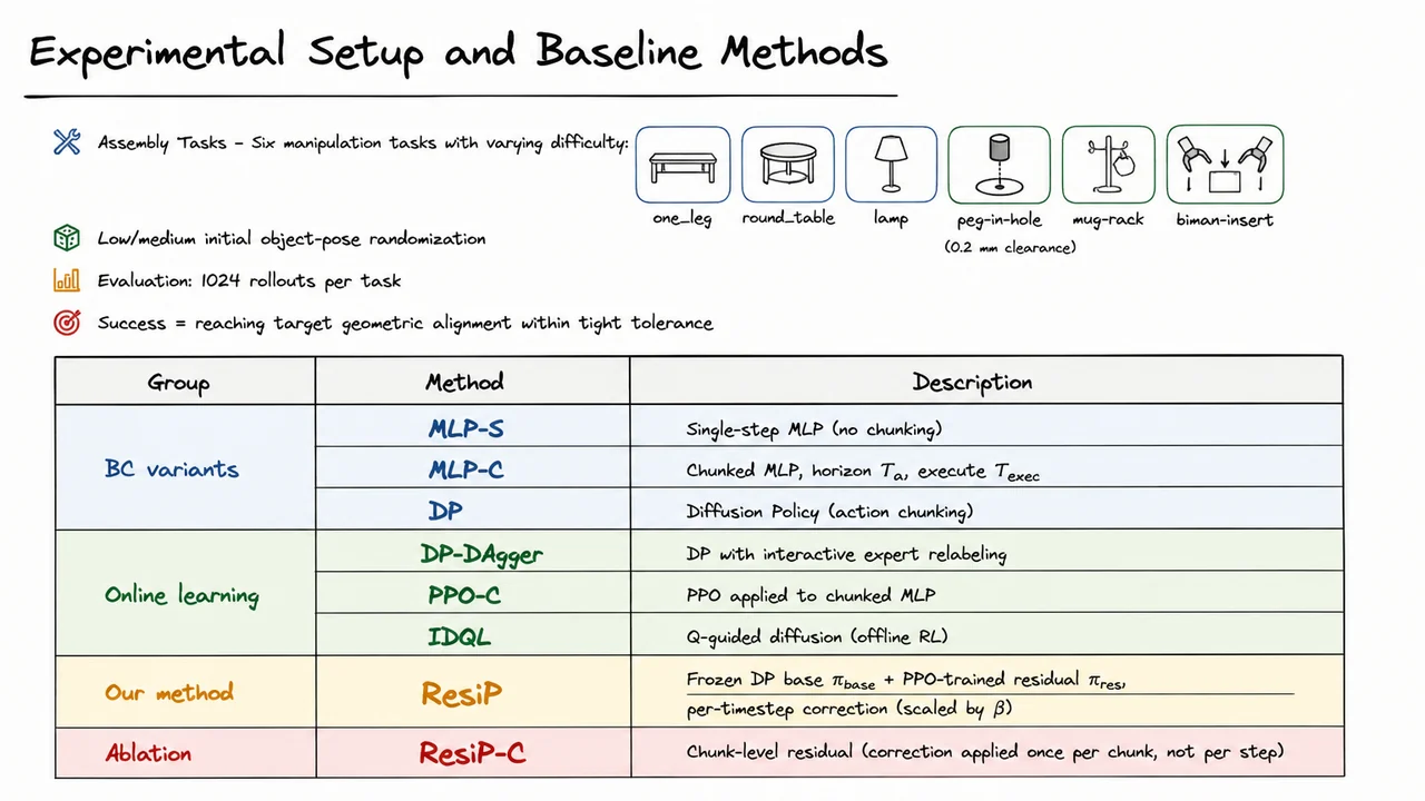
We evaluate on six dexterous assembly tasks that span a range of geometric complexity and required precision. They fall into two families:
one_leg), assembling a round table top onto its base (round_table), and fitting a lamp stem into its socket (lamp). These serve as a test of generalisation under moderate initial pose uncertainty.mug‑rack), and a challenging bimanual insertion (biman‑insert). Here the tolerance band is so tight that even a sub‑millimetre end‑effector drift leads to jamming or missed contacts.In every task, the initial object poses are randomised within a low‑to‑medium range, preventing the policies from memorising a single starting configuration. Performance is measured over 1024 rollouts per task, and success is defined strictly as achieving the target geometric alignment within the task‑specific tight tolerance. This protocol exposes brittleness mercilessly: a policy that performs well on a handful of hand‑picked seeds often collapses on the full distribution.
With the tasks fixed, we construct an exhaustive baseline matrix. The BC variants capture the spectrum from a plain single‑step MLP (MLP‑S) — no chunking, reacting purely to the current observation — to a chunked MLP (MLP‑C) that predicts a horizon and executes the first actions, and finally the full Diffusion Policy (DP) which uses a denoising diffusion process to generate action chunks of length . All BC variants are trained on the same expert demonstrations and share an identical observation space. The online learning group pushes into RL territory: DP‑DAgger interleaves deployment with interactive expert relabelling (a classic dataset‑aggregation scheme applied to the diffusion policy); PPO‑C uses Proximal Policy Optimization to directly train a chunk‑level policy (outputting one chunk per RL step); and IDQL represents a modern offline‑to‑online approach that guides a diffusion model with a learned Q‑function, fine‑tuned from static data. Our own method, ResiP, is deliberately minimal: we freeze the base diffusion policy exactly as produced by BC and then train, with PPO, a lightweight residual policy . At each control timestep, the robot state is fed to (which generates a chunk and executes its first action) and to (which outputs a correction vector). The correction is added to the base action after scaling by a factor , providing a per‑timestep, closed‑loop adjustment — but the heavy lifting of base action generation remains untouched. For ablation we also consider ResiP‑C, where the residual correction is computed once per chunk and held constant for steps, which isolates the value of per‑step feedback.
What sets ResiP apart is not a cleverer base policy or a larger model; it is the decoupling of what to do long‑term (the frozen chunk from ) and how to nudge each step (). This separation avoids the destructive forgetting and instability of full RL fine‑tuning while still allowing the policy to react to the instantaneous consequences of previous corrections.
The visual below distills this experimental design into a clean, colour‑coded table. Rows are grouped by category — behavioural cloning variants, online learning methods, our method, and the ablation — with each group receiving a distinct pastel background (light blue for BC, light green for online, light yellow for ResiP, and light red for the chunk‑level ablation). Method names are presented in bold, and the descriptions are trimmed to one or two essential sentences: MLP‑S as single‑step MLP, MLP‑C with chunk horizon and execution length , DP as Diffusion Policy, DP‑DAgger with interactive relabelling, PPO‑C as PPO on chunked MLP, IDQL as Q‑guided diffusion, and finally ResiP and ResiP‑C with their respective correction granularities. Above the table, a compact bullet list reminds the reader of the six assembly tasks and the 1024‑rollout success metric. This at‑a‑glance layout makes it immediate that every baseline is evaluated under identical conditions, and that the only axis of variation is the policy structure and training paradigm. It serves as both a reference card and a promise: the following results will compare these methods head‑to‑head, revealing precisely where residual, per‑timestep correction triumphs.
After establishing the baselines, we now turn to the central empirical question: can a simple, learned additive correction revive a frozen behavior cloning (BC) planner, pushing it from mediocre imitation to reliable, high‑precision assembly? The answer, as ResiP’s main results demonstrate, is a resounding yes—but the magnitude of the improvement is what truly stands out. Understanding why demands a brief recap of the failure modes that afflict conventional action‑chunking methods.
Diffusion‑based BC policies produce smooth, multi‑step action chunks that are globally sensible but locally fragile. When executed open‑loop—applying the first action, then shifting the chunk window—the policy never explicitly corrects for accumulated errors. Even small distribution shifts induced by slight initial pose variations or unmodeled dynamics cause the planned trajectory to drift, and without online feedback the robot cannot recover. Direct online RL fine‑tuning of the diffusion model sounds tempting, but the high‑dimensional action chunk space and the stochastic nature of diffusion make stable credit assignment notoriously difficult; the policy often forgets previously mastered behaviours or fails to improve beyond a saturation point. Residual RL offers a radically different strategy: freeze the BC planner as an expert sketch and train a compact closed‑loop corrector that acts at each timestep, transforming a brittle open‑loop execution into a robust, reactive controller.
In ResiP, the frozen BC base policy still generates a full action chunk from the current observation, but instead of blindly executing the chunk’s first action, the system augments it with a learned residual produced by a small multi‑layer perceptron . This residual policy conditions on the current state, the BC‑intended action, and optionally a short history of observations. The final action is executed in the environment, and the next observation is received before the next residual is computed—enabling continuous, per‑timestep correction. Because remains entirely frozen, it never suffers from catastrophic forgetting; its smooth, coarse‑grained plan acts as a strong attractor, while only needs to learn local refinements that bring the end‑effector into precise alignment. Training the residual policy with PPO is sample‑efficient because the exploration starts from a near‑successful trajectory, and the policy’s action space is low‑dimensional (typically just a few residual deltas) compared with the full action chunk.
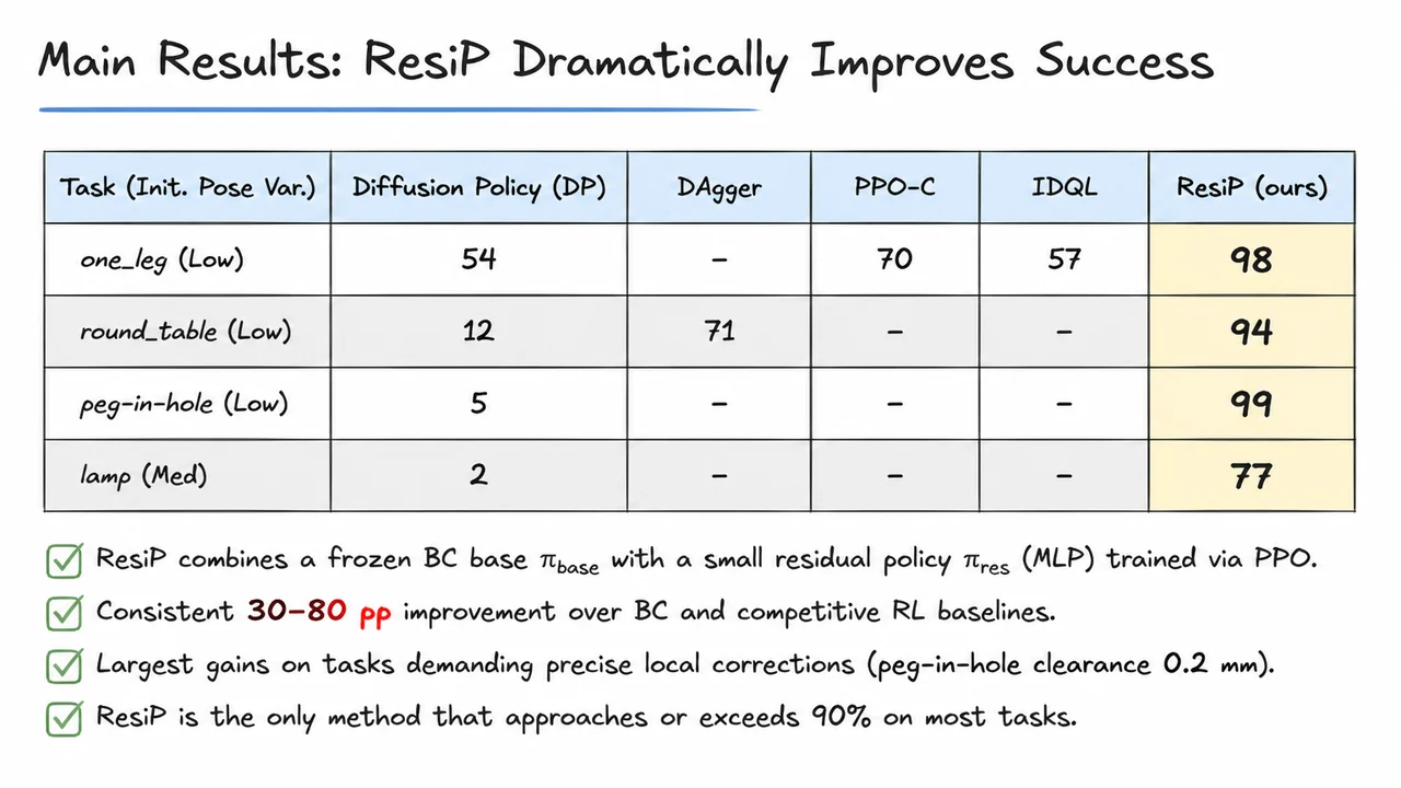
The practical impact of this design becomes immediately clear when we inspect success rates across four representative assembly tasks (Table I excerpt). The Diffusion Policy (DP) baseline, despite its strong open‑loop smoothness, collapses on tasks requiring sub‑millimetre accuracy: peg‑in‑hole with a 0.2 mm clearance sees a mere 5% success, while round_table and lamp achieve only 12% and 2% respectively. Other methods—DAgger, PPO‑C (RL applied directly to chunked actions), and IDQL—offer partial remedies, but none consistently break the threshold needed for reliable deployment. ResiP, by contrast, achieves 99% on peg‑in‑hole, 94% on round_table, and 77% on lamp. Even the one_leg task, where DP already reaches 54%, jumps to 98% with ResiP, a gain of 44 percentage points that underscores how per‑step refinement compounds over the episode.
These dramatic gains are not isolated outliers; they reflect a consistent pattern of 30–80 percentage point improvements over the strongest BC and RL baselines. The largest jumps occur on tasks that demand precise local corrections—exactly the regime where frozen BC chunks drift and where a purely open‑loop policy cannot self‑stabilize. ResiP’s closed‑loop nature turns the fragile chunk planner into a robust system: every timestep’s residual nudges the manipulator back towards success, absorbing initial pose variation and preventing the slow divergence that plagued DP. Notably, ResiP is the only method that surpasses 90% on most tasks, a success level that begins to look practical for real‑world assembly lines.
The visual below compresses this experimental story into an at‑a‑glance summary. The table lists the four tasks with their initial pose‑variation levels, followed by columns for DP, DAgger, PPO‑C, IDQL, and ResiP—the latter shown in bold with a warm yellow highlight. The numbers speak for themselves: ResiP’s column reads 98, 94, 99, 77, towering over the others. Beneath the table, three bullet points reinforce the takeaways: the consistent 30–80 pp lift, the exceptional gains on high‑precision insertion, and ResiP’s unique ability to reach near‑perfect or reliably high success rates. This visual encapsulation drives home the central message: residual RL doesn’t just incrementally improve a BC policy—it transforms a fundamentally flawed open‑loop chunk executor into a powerful closed‑loop system capable of mastering assembly tasks that seemed out of reach. The next piece of the puzzle, which we’ll explore shortly, is whether this per‑step correction also bestows resilience against dynamic disturbances that never appear in the training data.
The leap from a high success rate in controlled demonstrations to reliable performance in the real world is rarely a matter of better imitation alone. In the previous section, we saw that ResiP pushes assembly success to near-perfect levels when the environment behaves exactly as during training. Yet precision tasks, especially those involving tight insertions like snap-fits or gear meshing, are unforgiving: a small unexpected nudge during execution can derail a carefully choreographed motion plan. This brings us to a critical stress test—closed-loop robustness to dynamic disturbances. Rather than simply assessing static accuracy, we now ask whether a policy can react to sudden, mid-trajectory perturbations and still complete the task.
Dynamic disturbances—random forces applied to the manipulated object during execution—expose a fundamental limitation of action chunking approaches. Behavior cloning with chunked action prediction, whether via diffusion policies (DP, ) or dataset aggregation (DAgger), generates a multi-step action sequence at the start of each chunk and commits to it until the next re-planning opportunity. If the object is jostled partway through a chunk, the pre-computed actions become stale; the robot continues moving as if the object were still on its original trajectory, often missing the assembly target entirely. Because the policy only re-evaluates at chunk boundaries, the system behaves open-loop within each chunk, with a correction lag that can span several timesteps. The result is a brittleness that pure behavioral statistics cannot erase.
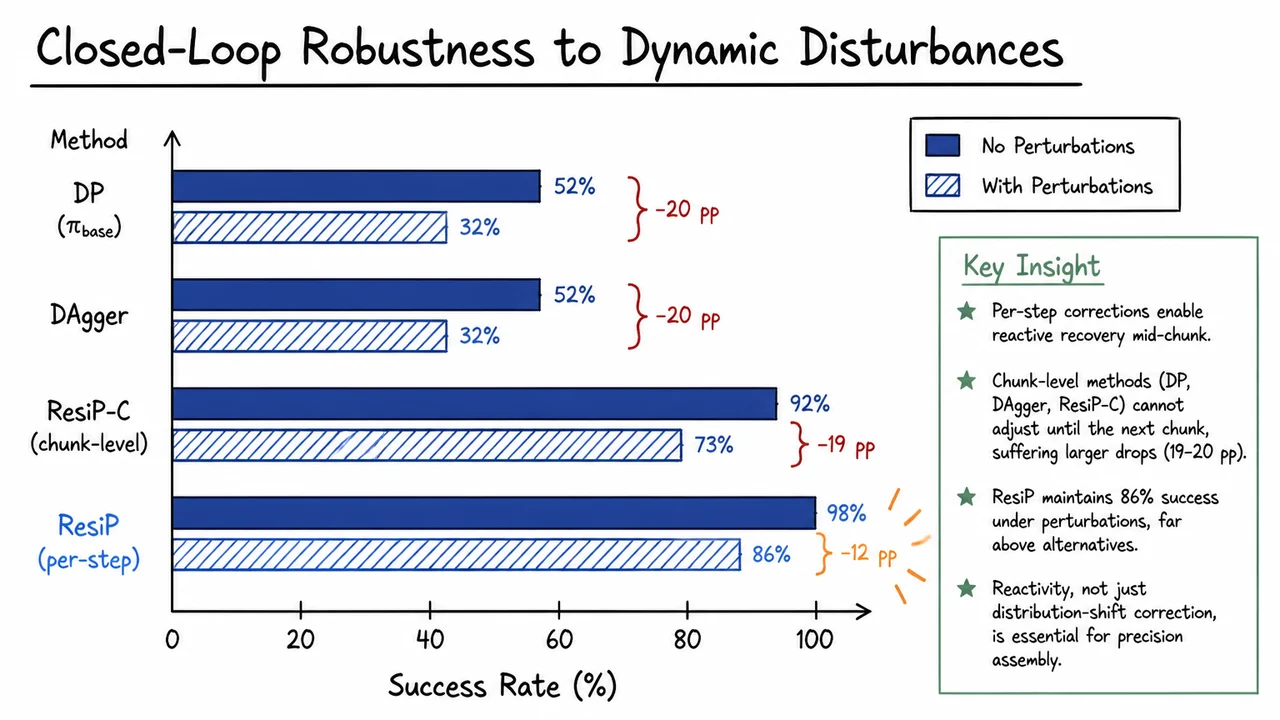
The same structural rigidity haunts chunk-level residual methods. ResiP‑C applies a residual correction to the entire chunk output of the frozen base policy, effectively nudging the planned action sequence in a more robust direction. However, that correction is still computed once per chunk and held constant throughout its execution. If a disturbance occurs mid-chunk, ResiP‑C has no mechanism to adapt until the next correction window. Consequently, its drop in success under perturbations is nearly identical to that of DP and DAgger: a sobering 19–20 percentage points. The level of success before disturbances is significantly higher (92% vs 52%), reflecting the power of residual fine‑tuning to fix chronic distribution shift, but the sensitivity to unexpected dynamics remains essentially unchanged.
This is where the per‑step residual formulation of ResiP becomes a qualitative leap forward. Because ResiP evaluates its residual policy at every timestep, it can inject a corrective delta into the base action immediately upon observing a state deviation. The frozen base chunk still provides a useful open‑loop prior, but the residual component acts like a high‑bandwidth feedback term: if the peg is knocked sideways, the per‑step residual can command a lateral recovery move within the same chunk, long before the next re‑planning cycle would normally occur. The reactive correction is not about learning an optimal trajectory from scratch; it is about learning a compact, state‑dependent repair signal that keeps the nominal plan aligned with the changing world.
The empirical numbers tell a story of resilience that matches this intuition. Under a standard perturbation regime—random forces applied at unpredictable moments and magnitudes—ResiP retains an 86% success rate, down only 12 percentage points from its unperturbed 98%. In contrast, every method that lacks per‑step reactivity suffers a success drop nearly twice as large. Notice that even ResiP‑C, which shares the same residual fine‑tuning objective but operates at the chunk level, sees its success fall from 92% to 73% (a 19‑point drop). The critical variable is not whether a method corrects for distribution shift (all residual variants do), but when those corrections are allowed to take effect. A 20‑step lag is an eternity when a millimeter off‑axis means a failed insertion.
The grouped horizontal bar chart on the slide distills this comparison into a single, scanable visual. Each method—DP, DAgger, ResiP‑C, and ResiP—is represented by a pair of bars: a solid bar for the unperturbed success rate and a lighter, hatched bar for the perturbed case. The vertical gap between the two bars of a pair visibly encodes the robustness penalty. For the first three methods, the drop is a conspicuous cliff, while for ResiP the hatched bar stays much closer to the solid one, with the gap drawn in a contrasting color. Annotation labels call out the exact percentage‑point decline, making the asymmetry between a 20‑point and a 12‑point penalty unmistakable even from the back of a lecture hall. The visual hierarchy reinforces the core message: superior steady‑state accuracy does not guarantee dynamic resilience; only temporally fine‑grained, closed‑loop correction can truly shrink that gap. By grounding the numbers in a clear spatial metaphor, the diagram lets the reader see that reactivity is not a secondary feature but the decisive factor for robust precision assembly.
After establishing that closed‑loop per‑timestep corrections give ResiP a decisive advantage against dynamic disturbances, a natural follow‑up is to strip the method down to its components and ask: what exactly is driving the performance? If we modify one piece at a time, do we still get the same gains, or does the system collapse under the precision demands of tight‑tolerance assembly? A rigorous ablation across four design axes answers these questions and reveals that ResiP’s success is not the result of a single clever trick, but of a carefully orchestrated interplay between architecture, reactivity, data, and scale of corrections.
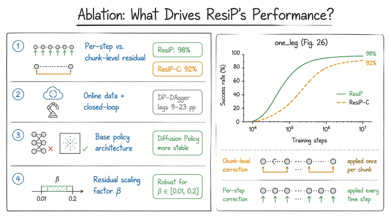
The first and most revealing axis compares per‑step versus chunk‑level residual correction. In a chunked behavior‑cloning setup, the base policy predicts a fixed‑length action chunk, which the robot executes open‑loop for its entire duration. ResiP introduces a residual policy that adds a small correction vector at every timestep, thereby closing the loop and allowing the robot to react to subtle misalignments as they appear. An obvious ablation is ResiP‑C, which instead applies a single chunk‑level residual correction — computed once per chunk — and holds it constant throughout the chunk. On the one_leg assembly task, this single design change drops the success rate from 98% down to 92%, and the learning curve shows markedly slower progress. The takeaway is unambiguous: high‑precision insertion tasks such as one_leg demand the ability to adjust forces and poses multiple times within a single chunk. A chunk‑level correction simply cannot react fast enough when the tolerances are sub‑millimeter, and the performance gap grows with task difficulty.
The second axis tackles a tempting but incomplete alternative: online data collection with closed‑loop execution, but no residual learning. Could we simply collect more online rollouts with a frozen BC policy and use DAgger‑style imitation to fix the observed mistakes? The experiment tests this via DP‑DAgger, which uses online data to continually refine a Diffusion Policy via BC without any residual RL. Across multiple tasks, DP‑DAgger still trails ResiP by 9–23 percentage points. This reinforces that the presence of online data alone does not automatically yield closed‑loop reactivity; the missing ingredient is a learned correction policy that can make fast, local adjustments per timestep. BC, even with online corrections, tends to average over noise and loses the ability to correct deviations that were not explicitly present in the corrective demonstrations. Residual RL, by contrast, is purpose‑designed to discover those small high‑reward actions that bring the end‑effector back on track.
The third axis concerns the base policy architecture itself. ResiP builds its residual policy on top of a frozen Diffusion Policy, which has already shown strong robustness when handling multimodal action distributions and exploration noise. If we swap out the Diffusion Policy for a simple deterministic MLP that directly outputs actions, the entire residual learning pipeline becomes unstable. The MLP base suffers training collapse even under medium environment randomness, because it cannot model the exploration‑induced distribution shift in the action space. The Diffusion Policy’s ability to generate diverse, denoised actions provides a smooth, explorable manifold over which the residual critic can safely learn. In essence, the base policy must already be robust enough to produce plausible actions under noise; otherwise the residual corrections amplify rather than refine erratic behavior.
The final axis examines the residual scaling factor : the scalar multiplier that scales the output of the residual policy before adding it to the base action. The findings show that performance is stable across a wide range . This insensitivity is important — it means the method does not require delicate tuning, and the constant itself serves a structural purpose: it encodes an inductive bias that keeps the residual corrections local. A small ensures that the base policy remains the primary driver, while the residual RL merely nudges the actions towards higher precision. Without this scaling, the residual policy might overwrite the base entirely, discarding the BC prior and leading back towards the brittleness of pure RL.
Stepping back, these four ablation axes paint a clear picture: ResiP’s headline‑grabbing 98% success rate does not arise from any single component but from the synergy of a Diffusion Policy base that handles exploration noise, per‑timestep reactivity provided by a residual policy, an online fine‑tuning loop that collects corrective data, and a scaling factor that respects the base policy’s expertise. Remove any of these — replace per‑step corrections with a chunk‑level equivalent, drop the residual learning in favor of online BC, use an MLP base, or let the residual dominate — and performance degrades sharply.
The accompanying visual consolidates these insights into a compact, digestible form. On the left, four framed bullet groups succinctly capture each ablation axis, each ending with a crisp quantitative result — for example, “ResiP‑C: 92% → ResiP: 98%” — making the causation immediate. The right side anchors the most critical comparison, per‑step versus chunk‑level correction, with an inset learning‑curve plot adapted from the paper’s Figure 26: the solid green ResiP curve arcs smoothly upward to ~98%, while the dashed orange ResiP‑C curve visibly saturates around 92%, visually encoding the reactivity gap. Below the plot, a miniature iconic diagram differentiates the two correction modes by contrasting a single block arrow applied once per chunk with many arrows applied at every timestep, reinforcing the core message without additional verbiage. The clean, hand‑drawn Excalidraw‑style aesthetic, accented by muted green for ResiP and neutral gray/orange for baselines, lets the reader scan the layout, absorb the four causal levers, and immediately see why per‑timestep closed‑loop corrections are indispensable.
The ablation study confirmed that ResiP’s strength lies in its closed‑loop residual corrections, which continuously adjust the base policy’s open‑loop chunk to meet tight assembly tolerances. But those experiments were performed in simulation with full access to object poses, wrench readings, and joint states—a luxury rarely available on a real robot that must rely on vision. The immediate practical question is therefore: how can we deploy a residual RL policy that was trained with privileged state information onto a real system that sees only raw pixels?
The standard BC recipe for vision‑based policies—collect a few human demonstrations and perform behavior cloning—struggles in high‑precision tasks for several reasons. Real demos are expensive, often noisy, and rarely cover the distribution of failures that emerge under closed‑loop execution. Moreover, an imitated open‑loop chunking policy can drift catastrophically when facing unseen lighting, background clutter, or object colors that violate the training distribution. To profit from the teacher’s near‑perfect residual actions without having access to the teacher’s state estimator, we need a strategy that transfers the teacher’s behavior across modalities.
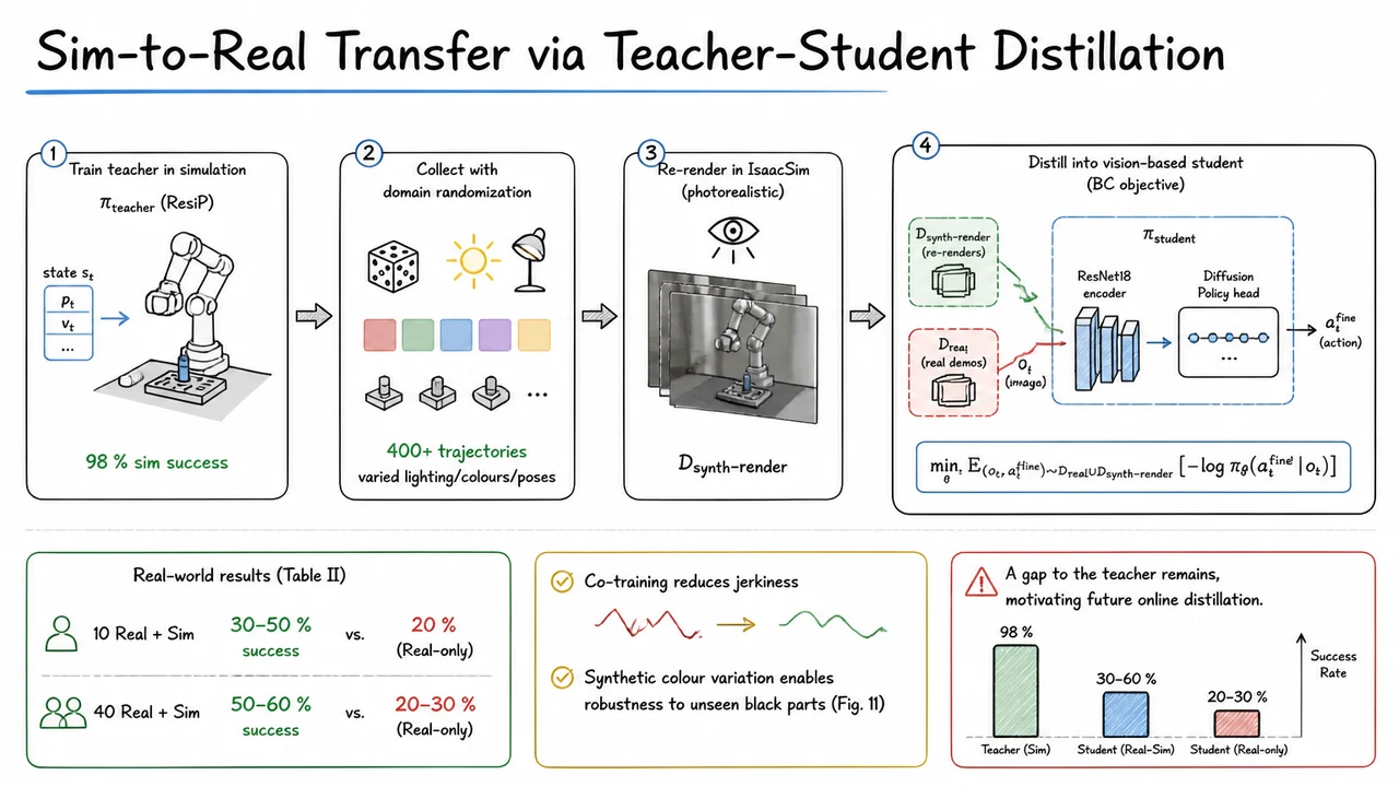
The teacher–student distillation framework presented here does exactly that. The key idea is to treat the state‑based ResiP teacher as an oracle that can generate virtually unlimited quantities of precisely labeled training data inside a simulator, and then to distill its closed‑loop corrective behavior into a vision‑based student policy using a form of offline imitation. Because the teacher runs in simulation we can easily collect hundreds of successful trajectories while applying aggressive domain randomization: lighting intensity and color, part colors, background textures, and object poses are randomly perturbed during data collection. This randomization exposes the student to a wide spectrum of visual conditions, encouraging it to learn visual features that are truly task‑relevant rather than spurious correlations.
A further gap remains: even randomized renderings from a fast simulation engine can look obviously synthetic—missing the specularities, pixel noise, and subtle shadows of a real camera. To close this visual domain gap, the logged simulation states are re‑rendered through a photorealistic renderer (IsaacSim) to produce . Each frame in this dataset is a high‑fidelity image paired with the corrective action that the teacher would have output at that timestep. This dataset, by itself, carries the teacher’s precision but still does not perfectly match the real‑world image distribution. Hence we also collect a handful of real‑world demonstrations —typically just 10 to 40 trajectories—where the robot is guided through the assembly under natural lighting.
The student policy (a Diffusion Policy paired with a ResNet‑18 visual encoder) is then trained by behavior cloning on the union of both datasets. The loss function is the standard negative log‑likelihood:
Crucially, the synthetic data supply precise corrective actions that reflect the closed‑loop refinement the teacher performs, while the real data anchor the visual encoder to authentic textures and backgrounds. This co‑training yields a dramatic boost. The results reported in the paper show that with only 10 real demonstrations and synthetic co‑training, real‑world success jumps to 30–50 %, compared to 20 % when training on the real demos alone. With 40 real demonstrations, success reaches 50–60 % versus 20–30 % without synthetic data. Anecdotally, the co‑training also yielded smoother trajectories (less jerkiness) because the synthetic data help the policy generalize over a broader range of visual appearances; notably, the policy became robust to an entirely unseen black part, a distribution shift that would have been catastrophic for a vision policy trained only on a handful of real trajectories with default colors.
Despite the strong improvement, a gap to the teacher’s 98 % simulation performance remains. The student, being a feed‑forward imitation of the teacher’s action sequence on re‑rendered images, may still suffer from mild covariate shift when deployed in a real loop, and it lacks the online adaptation that the teacher enjoyed. This motivates future work on interactive distillation (e.g., DAgger‑style data aggregation) or fine‑tuning with real‑world reinforcement learning.
The full pipeline is compactly summarized in the visual flow diagram below. Starting on the left, the state‑based ResiP teacher (achieving 98 % in sim) feeds a domain‑randomized data collection stage, where hundreds of trajectories are captured under varied lighting, colors, and poses. These are then re‑rendered with photorealistic fidelity to form the synthetic dataset . Together with a small stack of real demonstrations , the mixed data drive the distillation of the vision‑based student. The two callout boxes at the bottom report the success rates for different sizes of real demos, highlighting how synthetic co‑training increasingly lifts performance as the available real data grows. The inset referencing the unseen black part (Fig. 11) underlines how color randomization in simulation spills over into real‑world robustness—a concrete, high‑stakes benefit of the teacher–student design.
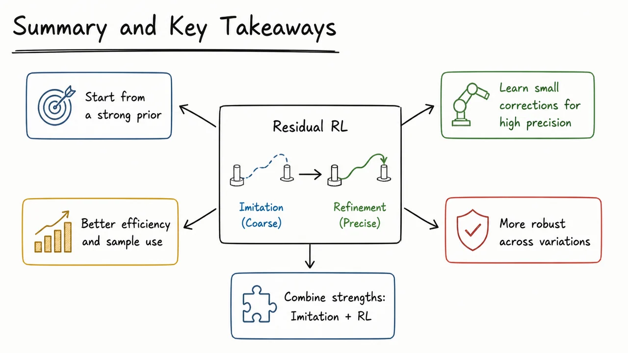
The previous section showed how a teacher–student distillation pipeline can transplant a carefully trained policy from a privileged simulation into a real-world vision-based system, preserving the refined behavior while adapting to raw sensor inputs. That final piece of the puzzle—making the leap from sim to real—sits on top of a deeper story: we began with a behavior-cloned policy that works passably well, but discovered it falters precisely when tasks demand high accuracy. By the end of the lecture, we arrive at a complete approach that transforms an imitation-learned base into a robust, closed-loop assembly agent. This final segment draws together the major threads, highlighting the core problems, the key insight behind residual reinforcement learning, and why the combination of imitation and refinement matters for real robotics.
The fundamental challenge starts with action chunking in behavior cloning (BC). Representing a trajectory as a sequence of predicted action chunks—such as a diffusion model that outputs 10–20 timesteps at once—makes the policy inherently open-loop over each chunk. Small prediction errors accumulate within a chunk because the policy cannot observe intermediate outcomes until the next replanning point. This creates a distribution shift: the policy is trained on expert demonstrations where chunks always stay close to the nominal distribution, but at test time it gradually drifts into states it has never seen, causing it to output increasingly erratic chunks. The result is a performance plateau far below the precision needed for tight-tolerance assembly; throwing more demonstrations at the BC problem does not fix the fundamental open-loop compounding error.
ResiP (Residual Policy learning) addresses this by keeping the frozen chunked BC policy as a strong, task-consistent prior and learning a residual policy that applies closed-loop corrections at every control timestep. Formally, if the BC policy produces a chunk , the executed action at step becomes
where is a small, learned residual that sees the current observation (including force-torque, pose error, etc.) and the nominal action from the BC chunk. The residual policy is trained with standard reinforcement learning, but its parameters are limited to keep it close to zero, preserving the BC’s structure while allowing fine-grained corrections. This bridges the gap between open-loop imitation and the reactive precision required for assembly: the BC prior supplies overall task guidance, while the residual handles per-timestep errors, slipping, and alignment drift.
An essential takeaway is why this residual fine-tuning is preferable to directly fine-tuning the entire diffusion or chunked policy with RL. When we unfreeze the whole BC policy and let RL tweak all its parameters, we risk catastrophic forgetting—the policy can rapidly diverge from the expert behavior and lose the general shape of the task, requiring huge amounts of environment interaction to recover stable behavior. In contrast, freezing the BC base and adding a small residual head is far more sample-efficient because the search space is constrained; the RL objective only needs to shape corrections, not rediscover the whole task. The residual acts as a safety net, never overriding the BC entirely, which also improves safety during on-policy data collection.
The closed-loop per-timestep nature of the residual policy is the critical factor behind the robustness gains. Instead of executing an entire open-loop chunk and hoping it remains valid, the agent observes sensory feedback after every action and makes micro-adjustments. This means if a grasped peg begins to tilt due to a slight misalignment, the residual immediately compensates with a small corrective torque; if contact forces spike, the residual can pull back slightly. The net effect is a dramatic increase in success rate for high-precision peg-in-hole and similar tasks, from BC baselines stuck below 50% to near-perfect insertion rates after residual training. Moreover, this reactive behavior transfers naturally to sim-to-real setups because the residual is conditioned on real sensor readings and can correct for unmodeled dynamics, friction, and vision noise, as long as the teacher policy guides the general assembly trajectory.
Bringing these ideas full circle, the sim‑to‑real pipeline discussed earlier makes the residual policy deployable in the real world. A privileged teacher (with ground‑truth state and force) trains the residual, and then a student network, operating solely on RGB images and wrist force-torque, distills the same corrective behavior through supervised regression on the teacher’s residual outputs. This two‑stage process ensures that the real‑world agent inherits the precision of closed‑loop corrections without needing privileged simulation state.
The accompanying visual consolidates this full journey from imitation to refinement. It sketches a branching flow: on the left, the BC agent producing a long action chunk that drifts away from the target, labeled with the failure mode of open‑loop compounding error; on the right, the ResiP solution where the same BC output is routed into a per‑timestep residual corrector that continuously adapts to sensor feedback, closing the loop. Central callouts compare the sample efficiency and robustness of residual RL versus direct fine‑tuning, while small icons hint at the teacher‑student distillation step that carries these corrections into a vision‑based real‑world policy. The diagram’s hand‑drawn aesthetic and sparse labels serve as a high‑level map of the lecture’s main message: by keeping what imitation does well and refining what it cannot, we build a precise, deployable assembly agent.