Speculative Decoding: Lossless Acceleration for Large Language Models

If you have ever waited for a large language model to generate a long response, you know the pain: the text appears token by token, each step draining precious milliseconds, yet the overall pace feels glacial. This sluggishness is not an accident of poor engineering; it is a direct consequence of the autoregressive decoding paradigm that almost every high-quality generative model uses today. To understand why, we need to unpack the underlying computational mechanics.

At each generation step, the model must evaluate the entire sequence of previously generated tokens to produce the next one. That means for token $x_t$, the model computes a forward pass over the full prefix $x_{<t}$, regaining the contextual representation that conditions the distribution $p(x_t \mid x_{<t})$. Because each new token depends on the complete state computed from the previous tokens, the decoding process is inherently sequential: you cannot start computing $x_{t+1}$ before you know $x_t$. The result is a cascade of forward passes that cannot be overlapped or batched across time steps.

For a concrete illustration, consider a large transformer with 175 billion parameters—the scale of models like GPT-3. Running a single forward pass through such a network is expensive; on modern hardware optimised for large language models, the per‑token latency $t_{\text{step}}$ often hovers around 50 milliseconds. The total wall‑clock time to generate a response of length $L$ is therefore given by a simple linear relation: $$\text{Latency} = L \cdot t_{\text{step}}, \qquad t_{\text{step}} \approx 50\,\text{ms}.$$ Plugging in realistic numbers yields a sobering figure: generating merely 100 tokens consumes more than 5 seconds. For interactive applications—chatbots, voice assistants, live coding assistants—this delay destroys the feeling of responsiveness and makes real‑time use impractical.

The intuitive urge is to parallelise the generation. If we could predict all $L$ tokens simultaneously, we would slash latency from $O(L)$ to $O(1)$ forward passes. Non‑autoregressive models attempt exactly that: they forgo the causal dependency and generate the whole sequence in one shot. But this shortcut comes at a steep price. Removing the sequential conditioning erases the precise causal structure that makes the target model’s output distribution $p(x_t \mid x_{<t})$ so accurate. The result is a model whose joint distribution over sequences differs from the original—often visibly in the form of incoherent, repetitive, or semantically broken text. So while non‑autoregressive methods are fast, they sacrifice exact quality, making them unsuitable when every token matters.

The challenge, therefore, crystallises into a strict requirement: we need an acceleration strategy that reduces the number of sequential costly forward passes without altering the output distribution one iota. That is, we must obtain samples $x_1, x_2, \dots, x_L$ such that each token is drawn exactly from $p(x_t \mid x_{<t})$ of the target model, but with a total computational budget far below $L$ expensive target‑model evaluations. This is the “lossless parallelisation” problem. Its solution is what this lecture series will introduce: speculative decoding—a paradigm that preserves the exact probability distribution while unlocking nearly order‑of‑magnitude speedups on long sequences.

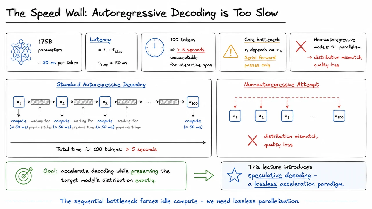
Before diving into the algorithmic machinery, it helps to visualise the nature of the speed wall and why naive attempts at parallelisation fail. The visual below is a conceptual diagram that dramatises the dilemma. On the left, we see a timeline of standard autoregressive generation: a horizontal chain of token boxes, each connected by arrows that force strict serial dependency, with conspicuous idle gaps between them representing the time spent waiting for a forward pass. The cumulative latency stretches past 5 seconds for just 100 tokens. On the right, a non‑autoregressive attempt appears: all tokens burst out almost simultaneously, but a bold red cross marks the result as “distribution mismatch, quality loss.” The contrast makes immediate the predicament: sequential execution yields exact quality but unbearable latency; naive parallelisation yields speed but destroys the very distribution we cherish.

This diagram is not just an illustration; it is a compact statement of the problem statement. The idle compute gaps in the autoregressive timeline are the hidden inefficiency that speculative decoding exploits. The red cross on the parallel attempt reminds us that we cannot simply discard the causal conditioning. Our journey will now lead us toward a principled strategy that pairs a fast, approximate draft model with the rigorous statistical backing of the target model to reclaim speed without surrendering a single bit of distributional fidelity.

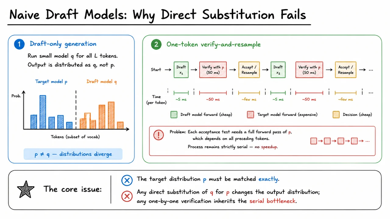
If autoregressive generation is the bottleneck, the most obvious escape route is to delegate the heavy lifting to a smaller, faster model. After all, a distilled or compressed draft model $q$ can sample token sequences with far lower per-step latency, and if $q$ approximates the target distribution $p$ reasonably well, the output might still be useful. The temptation is to simply let $q$ run for all $L$ tokens and present its result as though it came from $p$. This draft-only generation is the first naive attempt—and it collapses under a fundamental requirement: the final sequence must be an exact, unbiased sample from $p$. When we bypass the large model entirely, every token is drawn from $q$ instead; the output distribution is precisely $q$, not $p$. However well $q$ may mimic $p$ on average, distributional discrepancies inevitably creep in. Modes are suppressed, rare but plausible tokens vanish, and the long-tail coherence guaranteed by $p$ disintegrates. Using a draft model alone distorts the output, sacrificing the very quality we built the large model to provide. Speed gains come at the cost of correctness, and for many applications—factual generation, safety-critical replies, or faithful code synthesis—that trade-off is unacceptable.

A second naive attempt tries to salvage correctness by interleaving the draft and target models: generate one token with $q$, then verify it with $p$ before proceeding. The mechanics are simple in outline:

1. Draft-only generation — use $q$ to sample $L$ tokens; then check whether the whole sequence would have been produced by $p$. This degenerates to an expensive quality estimation step, not a speedup.
2. One-token verify-and-resample — for each position $i$, draft $x_i$ from $q$, compute the full conditional distribution $p(\cdot\mid x_{<i})$ from the large model, and decide whether to accept $x_i$ or resample from $p$ based on some rule.

At first glance, verify-and-resample seems safe because the large model is consulted at every step. However, the protocol inherits the very serial dependency that caused the speed wall. To compute $p(\cdot\mid x_{<i})$, the target model must process the entire prefix $x_{<i}$, which includes all previously accepted tokens. This means each verification step is a full forward pass through $p$—and it cannot start until the previous token is finalized. The loop looks like: draft $\rightarrow$ run $p$ (50 ms) $\rightarrow$ accept/resample $\rightarrow$ draft $\rightarrow$ run $p$ again. The per-token latency is now worse than pure autoregressive decoding with $p$ alone, because we add the cost of $q$ on top, and we still perform exactly $L$ target-model evaluations. The total time is $L \times (\text{draft cost} + \text{target cost})$, offering no parallelism and no net acceleration.

Underneath both failures lies a deeper invariant: any acceleration method must produce tokens that are identically distributed as an autoregressive sample from $p$. Exactness is non-negotiable for lossless speedup. The draft-only approach loses exactness by substituting $q$ for $p$. The one-token verify-and-resample approach preserves exactness (with an appropriate acceptance rule) but remains strictly sequential. The challenge, then, is to design a protocol that breaks the serial coupling while still guaranteeing that the final output is a valid sample from $p$. This is precisely the puzzle that speculative decoding solves, as we will see shortly.

The visual below consolidates these two failure modes in a compact, evidence-oriented format. On the left, a side-by-side bar chart compares the token probability distributions of $p$ (blue) and $q$ (orange) over a small vocabulary subset. The mismatch is immediate: peaks are located at different tokens, and some tokens are heavily over- or under-represented by $q$. This mirrors the core problem of draft-only generation—the output distribution simply does not match $p$. On the right, a timeline plot of the one-token verify-and-resample approach shows a flat, step-by-step sequence of “Draft $x_1$” → “Verify with $p$ (50 ms)” → “Accept/Resample” → “Draft $x_2$” → … , with each block labeled by its function. A dashed horizontal line representing the latency of pure autoregressive decoding emphasizes that this naive scheme offers no advantage; it in fact slightly increases total latency because each token incurs both a draft and a target evaluation. The diagram makes visible that distribution mismatch and serial dependency are two sides of the same coin: any scheme that insists on one-by-one verification cannot escape the speed wall, while any scheme that skips verification loses fidelity. Speculative decoding must, and does, navigate between these extremes.

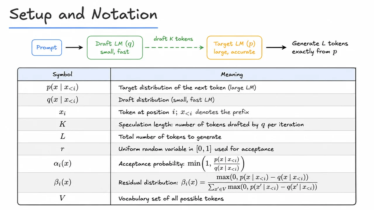
The observation that directly substituting draft tokens produces systematic drift from the target distribution makes one thing clear: a correct acceleration scheme must do more than just run a small model in place of the large one. It must actively correct for the mismatch between the small model’s predictions and what the large model would have predicted, while still leveraging the speed advantage of the small model. The core of speculative decoding is a carefully designed accept/reject routine that accomplishes exactly this, and that routine is fundamentally a statistical procedure built on rejection sampling. To state it precisely and later prove its correctness, we need a crisp, shared set of notation and definitions. This section lays out every symbol, every distribution, and every acceptance rule that the algorithm will use; it is the reference point for every equation and proof that follows.

We work with two autoregressive language models, both defining probability distributions over the next token given a prefix. The target model $p$ is the large, high‑quality model whose output we want to produce. Because computing $p(x_t \mid x_{<t})$ for every step is expensive, we also have a draft model $q$, which is much smaller and faster but generally less accurate. Both models are defined over a finite vocabulary $V$ (e.g., the tokenizer’s vocabulary of tens of thousands of tokens). For any prefix $x_{<i} = (x_1, \dots, x_{i-1})$, the conditional distributions $p(\cdot \mid x_{<i})$ and $q(\cdot \mid x_{<i})$ are probability mass functions over $V$. The goal is to generate a sequence of $L$ tokens $x_1, \dots, x_L$ that is distributed exactly according to $p$, but to do so with much lower average latency than a naïve autoregressive evaluation of $p$ at every step.

The speed gain comes from letting the draft model $q$ “look ahead” and propose several tokens in a single batch. We define the speculation length $K$ as the number of tokens the draft model generates in one go before the target model intervenes to verify and possibly correct the sequence. A typical value of $K$ might be 3–5 in practice; larger values can yield more speedup if the draft model is accurate, but they also increase wasted computation if drafts are frequently rejected.

Now, what happens when the draft model proposes a token $x$ at position $i$? We cannot simply keep it; we must decide whether to accept it as if it had been drawn from $p$. The decision is made by a random acceptance test that mimics a rejection sampler. For any token $x$ that $q$ produces, we define the acceptance probability

$$\alpha_i(x) = \min\!\left(1,\; \frac{p(x\mid x_{<i})}{q(x\mid x_{<i})}\right).$$

This says: if the draft model assigns too much probability to $x$ compared to the target model ($q(x\mid x_{<i}) > p(x\mid x_{<i})$), we accept with probability $p/q < 1$, thereby reducing the effective frequency of that token so that it matches the target. If the draft model assigns too little probability ($p(x\mid x_{<i}) \ge q(x\mid x_{<i})$), we are eager to accept the token because it is “safe”; the acceptance probability is 1 because the ratio exceeds 1 and the $\min$ caps it. However, when we always accept a token whenever $p \ge q$, we have not yet accounted for the extra probability mass that $p$ places on that token beyond $q$. That mass must be recovered later, at the first position where a draft token is rejected.

This need gives rise to the residual distribution $\beta_i$. Suppose we reach position $i$ and the acceptance test fails for the draft token. The algorithm then rejects all draft tokens from position $i$ onward and must produce a fresh token for position $i$ that is drawn from the part of the target distribution not yet covered by the draft model’s proposal process. Intuitively, the probability that a particular token $x$ should be the reset token is proportional to how much target probability mass $p(x\mid x_{<i})$ exceeds the draft probability $q(x\mid x_{<i})$ — the leftover mass that was “unused” because the draft model underestimated its likelihood. We therefore define

$$\beta_i(x) = \frac{\max\!\bigl(0,\; p(x\mid x_{<i}) - q(x\mid x_{<i})\bigr)} {\sum_{x'\in V} \max\!\bigl(0,\; p(x'\mid x_{<i}) - q(x'\mid x_{<i})\bigr)}.$$

The denominator normalizes the excess masses into a valid probability distribution over $V$. When the algorithm samples a reset token from $\beta_i$ after a rejection, it probabilistically restores the missing mass and, together with the earlier acceptance rule, guarantees that the final output is an exact sample from $p$.

All the accept/reject steps use a uniform random variable $r$ drawn independently from the interval $[0,1]$. In the final algorithm (to be detailed in the next sections), for each draft token $x_i$ we sample $r \sim \text{Uniform}(0,1)$ and accept $x_i$ only if $r < \alpha_i(x_i)$. If the inequality fails, we reject $x_i$, resample from $\beta_i$, and discard the remaining draft tokens.

The visual below provides a compact reference table that consolidates all of these symbols and their meanings. By separating the notation into a clean two‑column layout, it allows the reader to quickly recall the precise definition of every quantity before diving into the algorithm’s pseudocode or the proof of correctness. The table lists the target distribution $p$, the draft distribution $q$, token positions, the speculation length $K$, the total generation length $L$, the uniform random variable $r$, the acceptance probability $\alpha_i(x)$ with its formula, the residual distribution $\beta_i(x)$ with its formula, and the vocabulary $V$. All terms use consistent LaTeX notation, mirroring exactly the definitions we have just discussed. This visual summary will serve as a persistent reference as the lecture progresses from the high‑level idea to the rigorous acceptance/rejection logic.

The crippling latency of large language models stems from a basic fact about autoregressive generation: each new token must wait for the model to compute a full forward pass conditioned on all previous tokens. If we need to produce a sequence of length $L$ with an expensive target model $p$, we pay the cost of $L$ serial forward passes. No amount of batching or clever GPU scheduling can break this sequential dependency when we insist on sampling tokens one by one directly from $p$. Naive attempts to parallelize within a sequence fail because the state at step $i$ depends on the token actually chosen at step $i-1$; guessing multiple future tokens without verifying their joint likelihood would produce gibberish whose distribution diverges from the target.

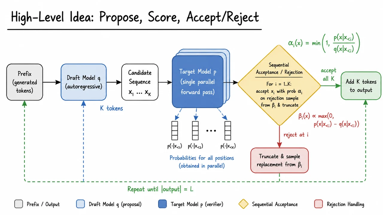
Speculative decoding circumvents this dilemma with a delightfully game-like strategy: propose, score, accept/reject. Instead of letting the expensive model $p$ do all the work, we employ a cheap, fast draft model $q$ to hastily scribble a few words ahead. The draft model, running autoregressively, suggests a candidate chunk of $K$ tokens $x_1,\dots,x_K$ that extend the existing prefix. Because $q$ is much smaller (or even a distilled version of the target), drafting $K$ tokens costs a fraction of what a single target‑model forward pass would. The crucial insight is that we can now verify that entire candidate sequence with the target model in one parallel forward pass. By feeding the full prefix‑plus‑candidates into $p$, we obtain the target probability vectors $p(\cdot \mid x_{<i})$ for all positions $i=1,\dots,K$ simultaneously – a luxury not available when generating token by token.

The final stage, sequential acceptance, is where the statistical magic happens. Simply appending the draft tokens would corrupt the output distribution; we need a rule that discards some tokens and replaces others so that the overall stream is indistinguishable from pure autoregressive sampling from $p$. The rule is a direct application of rejection sampling principles, but tailored to the sequential, prefix‑dependent nature of language generation. For each position $i$ from $1$ to $K$ we look at the candidate token $x_i$ that $q$ proposed. We accept it with probability

$$\alpha_i(x_i) = \min\!\left(1,\; \frac{p(x_i \mid x_{<i})}{q(x_i \mid x_{<i})} \right).$$

This is the classic accept‑probable‑enough test that guarantees the accepted tokens follow an effective distribution $\min(p, q)$. When $q$ overestimates a token (i.e., $q(x) > p(x)$), acceptance probability is less than one, correctly tamping down the overshoot. When $q$ underestimates, $\alpha_i = 1$ and we always keep the token, but this alone leaves a deficit: we haven’t generated all the probability mass that $p$ assigns to tokens for which $p(x) > q(x)$. That deficit is exactly $\max(0, p(x \mid x_{<i}) - q(x \mid x_{<i}))$, and after renormalization it becomes the residual distribution:

$$\beta_i(x) \propto \max\!\big(0,\; p(x \mid x_{<i}) - q(x \mid x_{<i})\big).$$

If at step $i$ we reject the draft token (which happens with probability $1 - \alpha_i$), we immediately sample a replacement from $\beta_i$. That replacement token fills the missing probability mass precisely, ensuring that the overall chance of finally emitting any token $x$ at position $i$ is exactly $p(x \mid x_{<i})$ – the same as the target model’s own sampling. Moreover, once a rejection occurs, the draft tokens after position $i$ were conditioned on a prefix that is now invalid (the replacement token differs from the original draft token at $i$), so we must truncate everything beyond $i$ and restart drafting from the new extended prefix.

This one‑iteration procedure – draft $K$ tokens, verify all in one $p$‑pass, scan left to right accepting or rejecting – repeats until we’ve produced the desired $L$ tokens. The average length of the accepted prefix depends on how closely $q$ tracks $p$. If the draft model is a good approximation, most tokens are accepted and each iteration nets nearly $K$ new tokens for the cost of a single target‑model forward pass (plus the cheap drafting cost). The algorithm is lossless: the token sequence is exactly distributed according to the target model $p$, as can be proved by showing that the process’s generative probability for any prefix of length $\ell$ equals $p(x_1^{\ell})$; the acceptance‑resampling rule acts as a perfect statistical corrector.

The accompanying diagram (Figure 4) crystallizes these ideas into a readable flowchart. The prefix enters the light‑blue draft model, which emits a candidate chain of $K$ tokens. That chain flows into the dark‑blue target model block, which sits on a parallel‑computation icon to emphasize that all positions are scored at once. The probability vectors then feed a yellow decision diamond labelled “Sequential Acceptance / Rejection”, where the acceptance probability $\alpha_i$ and the residual distribution $\beta_i$ operate step by step. A branch shows that full acceptance of all $K$ tokens loops back to the draft stage with an extended prefix, while a rejection at position $i$ triggers truncation, residual sampling, and a fresh draft. The dashed loop arrows make the iterative nature explicit, reminding us that the ballet of propose, score, and accept/reject continues until the output reaches its target length. This snapshot – one iteration in a single image – provides the mental map needed for the detailed step‑by‑step pseudocode that follows.

Having spent the last section understanding the high‑level plan of proposing, scoring, and accepting, we can now build the precise mechanism for one iteration of speculative decoding. This is the engine that turns a fast but imperfect draft model into a reliable source of tokens, all while respecting the target distribution $p$ exactly. Every detail—which tokens are drawn, when we stop, and what we do after a rejection—has been carefully chosen so that the final output is lossless: indistinguishable from tokens generated by a slow autoregressive call to $p$.

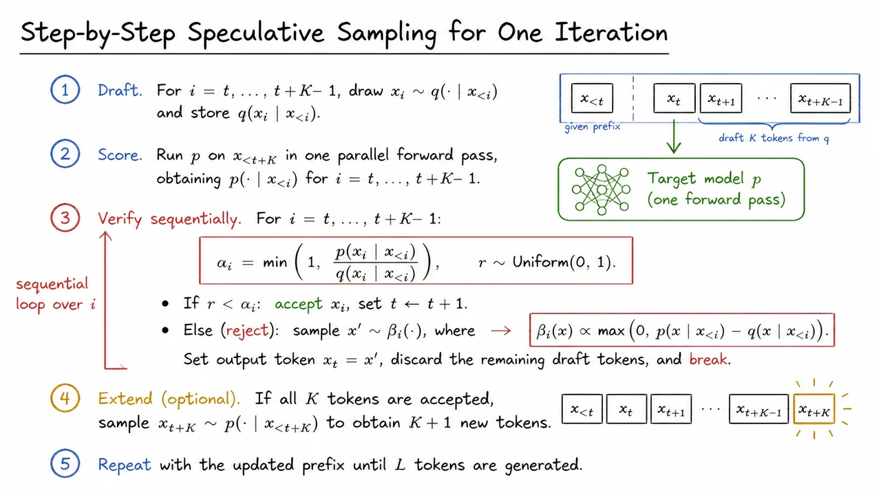
The iteration starts with an already‑decoded prefix $x_{<t}$. Instead of requesting one token at a time from the large model, we let a lightweight draft model $q$ propose a short sequence of $K$ tokens. Specifically, for each step $i = t,\dots,t+K-1$, we sample
$$x_i \sim q(\,\cdot\mid x_{<i}\,),$$ and we must remember the probability $q(x_i\mid x_{<i})$ that the draft assigned to that token. Sampling (rather than greedily picking the argmax) is essential here, because the later acceptance step needs the numerical probability ratio to make a correct correction.

Once we have a hypothesis $x_t, x_{t+1}, \dots, x_{t+K-1}$, we can invoke the target model $p$ once, in a parallel forward pass over the concatenated sequence $x_{<t+K}$. This batched evaluation gives us all the conditional probabilities $p(\,\cdot\mid x_{<i})$ for $i=t,\dots,t+K-1$ in the time that a single token would normally take. The dramatic speed‑up of speculative decoding lives in this single step: the draft tokens are cheap, and the expensive model sees them all at once. Now we have two distributions per position: the draft’s $q$ and the target’s $p$. The next task is to decide which draft tokens to keep.

That decision happens in a sequential verification loop that walks forward through the proposed tokens. For each position $i = t, t+1, \dots, t+K-1$, we compute an acceptance ratio
$$\alpha_i = \min\!\Bigl(1,\; \frac{p(x_i\mid x_{<i})}{q(x_i\mid x_{<i})}\Bigr),$$ and draw a uniform random number $r \sim \text{Uniform}(0,1)$. If $r < \alpha_i$, we accept the draft token $x_i$, advance the prefix (effectively $t \leftarrow t+1$), and move on to verify the next token. This rule looks like standard rejection sampling, but with a crucial twist: the envelope constant is taken to be $1$, so the acceptance probability is simply $\min(1, p/q)$. Because we process tokens one by one and condition on previous acceptances, the overall procedure maintains a delicate balance that keeps the final token distribution exactly $p$.

If the uniform draw exceeds $\alpha_i$, we reject the token. But we cannot just stop there, because we must still output a token that obeys the target distribution given the prefix. This is where the residual distribution comes in: $$\beta_i(x) \propto \max\bigl(0,\; p(x\mid x_{<i}) - q(x\mid x_{<i})\bigr).$$ In words, $\beta_i$ concentrates its probability mass exactly on those tokens where the target model assigns higher probability than the draft—the “correction” needed to make up for the shortfall when the draft’s proposal is not good enough. We sample a fresh token $x' \sim \beta_i(\cdot)$, set this token as $x_t$, and then discard the remaining draft tokens and break the loop. The algorithm effectively says: “The draft got this one wrong; we fix it with a corrected sample and we stop speculating further this step.”

Why does this work? A compact probability argument shows that for any position $i$, the marginal probability that the algorithm outputs a token $y$ — whether by acceptance or by rejection followed by resampling — equals $p(y\mid x_{<i})$. If $y$ was the draft token, the contribution is $q(y)\cdot \min(1, p(y)/q(y)) = \min(p(y), q(y))$. If the procedure rejects (whatever the draft token was) and then samples from $\beta_i$, the probability of obtaining $y$ is proportional to $\max(0, p(y)-q(y))$. Summing the two cases recovers exactly $p(y)$. This rejection‑sampling‑inspired coupling is the mathematical core that guarantees the method is lossless.

After the verification loop finishes (either naturally because all $K$ tokens were accepted, or prematurely because of a rejection), one small optional step remains. If the entire draft of length $K$ survived, we can extend the sequence by sampling one more token directly from $p$ at position $t+K$. This yields a total of $K+1$ new tokens in this iteration and ensures that even when the draft model perfectly mirrors the target, we always make progress and never get stuck with exactly the same output as the draft. The updated prefix then feeds into the next iteration, and the whole process repeats until the full sequence of length $L$ is generated.

The image below captures this complete single‑iteration workflow in a clean, structured visual. It enumerates the main phases—Draft, Score, Verify—with the central acceptance criterion displayed prominently, and it marks the sequential loop with a vertical arrow on the left, exactly as you would draw it on a whiteboard. The two bullet cases under “Verify” mirror the accept/reject decision, and the residual distribution $\beta_i$ is shown in its own display equation, clarifying where corrected samples come from. This kind of mixed text‑plus‑equation layout turns the four‑step recipe into a reference that students can revisit quickly after they have absorbed the deeper rejection‑sampling justification.

In speculative decoding, the draft model suggests a token $x$ drawn from its own distribution $q(x)$, but our goal is to produce a token that follows the target model’s distribution $p(x)$ exactly. The previous discussion showed how we can iterate over draft tokens, using the target model to score them in parallel, but it left open the critical decision rule: when do we keep the draft token, and what do we do when we must reject it? The answer lies in designing an acceptance criterion that makes the overall output distribution match $p$, while also keeping the rejection rate as low as possible to preserve the speed gains of drafting. This is the heart of lossless speculative sampling.

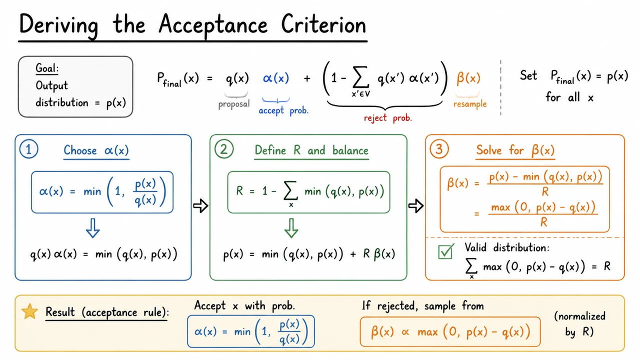
We can think of the token output process as a two‑stage mixture. Given a draft token $x \sim q$, we flip a biased coin that accepts it with probability $\alpha(x)$; if we reject, we forget $x$ and resample a replacement token from a separate residual distribution $\beta(x)$. The probability that the final output token equals a particular value $x$ is therefore

$$P_{\text{final}}(x) = q(x)\,\alpha(x) \;+\; \bigl(1 - \sum_{x'} q(x')\,\alpha(x')\bigr)\,\beta(x).$$

The first term accounts for the event where the draft token is $x$ and it is accepted. The second term accounts for cases where we reject whatever token the draft model proposed (this happens with probability $1 - \sum_{x'} q(x')\alpha(x')$) and then independently sample a new token from $\beta$, which could be $x$. For the overall process to be lossless, we must have $P_{\text{final}}(x) = p(x)$ for every token in the vocabulary $V$.

This condition alone is not enough to pin down $\alpha$ and $\beta$ uniquely; we have many degrees of freedom. The key insight is that we want to accept the draft token as often as possible because every acceptance means we save a costly target‑model sampling step. The tightest constraint is that the accepted‑draft term cannot exceed the target probability for any token—otherwise the residual term would need to be negative to balance the equation, which is impossible. Thus we must satisfy

$$q(x)\,\alpha(x) \le p(x) \quad \text{for all } x.$$

To maximize acceptance, we set $\alpha(x)$ as large as this inequality permits while also respecting the requirement that a probability cannot exceed 1. This gives the natural choice

$$\alpha(x) = \min\!\Bigl(1,\; \frac{p(x)}{q(x)}\Bigr).$$

When $q(x) \le p(x)$ (the draft model underestimates the target’s mass on a token), we can accept it always because the shortfall will be corrected by the residual component. When $q(x) > p(x)$ (the draft model over‑assigns probability), we must reject with enough frequency to bring the overall chance of outputting $x$ down to $p(x)$. The acceptance probability then scales as the ratio $p(x)/q(x)$, exactly mirroring the classic acceptance‑rejection sampling test from Monte Carlo methods.

Substituting this $\alpha(x)$ back into the mixture makes the first term simply $\min(q(x), p(x))$. Define the total acceptance probability across all tokens as

$$A = \sum_{x} q(x)\,\alpha(x) = \sum_{x} \min(q(x), p(x)).$$

The overall rejection probability is therefore $R = 1 - A$. The mixture equation now reads

$$p(x) = \min(q(x), p(x)) + R \,\beta(x),$$

which forces the residual distribution to be

$$\beta(x) = \frac{p(x) - \min(q(x), p(x))}{R} = \frac{\max(0,\, p(x) - q(x))}{R}.$$

Notice that the numerator is exactly the amount by which the target model places more probability on a token than the draft model does—the deficit we must recover. Summing these positive differences over all tokens yields

$$\sum_{x} \max(0, p(x)-q(x)) = 1 - \sum_{x} \min(q(x), p(x)) = R,$$

confirming that $\beta$ is a valid probability distribution. So when we reject a draft token, we resample from the set of tokens where the target model is more confident than the draft model, weighted by that excess. This elegantly corrects the bias introduced by the draft model’s inaccuracies.

The visual below distills this derivation into a three‑stage flow, making the algebraic relationships instantly legible. It begins with the declared goal that every output token must follow $p(x)$ and displays the mixture equation for $P_{\text{final}}$. Three connected boxes then walk through the logic: first, the choice $\alpha(x)=\min(1,p/q)$ is translated into $q\alpha = \min(q,p)$; second, the definition of $R$ as the residual mass sets up the balance equation; and third, solving for $\beta$ yields the formula $\beta(x) = \max(0,p-q)/R$ together with a verification that its total mass equals $R$. Arrows link the boxes to trace the reasoning, while the final banner—colored with blue for the acceptance rule and orange for the residual distribution—captures the only two formulas that will be executed at each token position in the speculative decoding loop. This compact view anchors the theoretical derivation before we turn to the formal correctness theorem that follows.

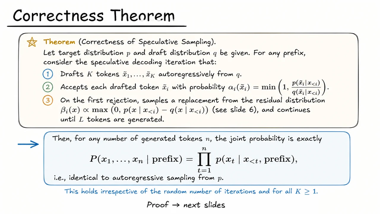
Having derived the acceptance criterion that decides the fate of each draft token, we now confront the question that ultimately determines whether speculative decoding is a viable acceleration strategy: does this iterative accept‑reject procedure actually produce tokens from the target distribution $p$? The whole scheme hinges on the guarantee that the accelerated generation is indistinguishable from a standard autoregressive sampling run. If speculative decoding were merely an approximation, any speed gains would come at the cost of quality degradation, a trade‑off rarely acceptable in practice. The correctness theorem formalises the remarkable claim that no such trade‑off is necessary.

The theorem states a clean, probabilistic equality. For any prefix (the context already generated), we consider the speculative decoding loop: the draft model $q$ proposes up to $K$ tokens $\tilde{x}_1,\dots,\tilde{x}_K$ autoregressively; each drafted token $\tilde{x}_i$ is accepted with probability $\alpha_i(\tilde{x}_i) = \min\!\bigl(1, \frac{p(\tilde{x}_i \mid x_{<i})}{q(\tilde{x}_i \mid x_{<i})}\bigr)$; and on the first rejection, a replacement token is drawn from the residual distribution $\beta_i(x) \propto \max(0, p(x \mid x_{<i}) - q(x \mid x_{<i}))$. The claim is that after an arbitrary number of generated tokens $n$, the joint probability of the sequence $x_1,\dots,x_n$ under this speculative procedure is exactly

$$P(x_1,\dots,x_n \mid \text{prefix}) = \prod_{t=1}^{n} p(x_t \mid x_{<t}, \text{prefix}),$$

the same product of conditional probabilities one would obtain by running the target model $p$ autoregressively from the start.

Why is this statement so important? Because it asserts that speculative decoding is lossless with respect to the target distribution. The generated text is not merely similar in some loose statistical sense; it is a valid sample from exactly the same distribution that an expensive, token‑by‑token invocation of the target model would produce. This holds for any draft model $q$, regardless of how poorly it approximates $p$, and for any choice of $K \ge 1$. The only price paid for a badly aligned draft model is a drop in acceptance rate—and therefore speed—but never a deviation from the target distribution. The theorem thus elevates speculative decoding from a clever heuristic to a principled acceleration technique.

The theorem’s scope is broader than it might first appear. It does not merely claim that the marginal distribution of each token matches $p(\cdot \mid \text{prefix})$ at the moment it is produced. That would already be a strong guarantee, but the theorem goes further: the entire sequence, with all its temporal dependencies, follows the distribution that the target model would assign. In other words, the accept‑reject mechanism preserves the full autoregressive structure of $p$. This is essential for coherence and long‑range consistency, as language models are not collections of independent letter generators but are defined by the way each token conditions on its entire history.

The proof of the correctness theorem proceeds in stages. First, one shows single‑token correctness: that in a single speculative step (drafting $K$ tokens, possibly accepting some and replacing at the first rejection), the next token that is finally appended to the prefix is distributed exactly as $p(\cdot \mid \text{prefix})$. This is a direct consequence of the rejection‑sampling logic we derived in the previous sections: the acceptance rule ensures that any token $x$ from $q$ is admitted with the right probability to make the accepted token exactly $p$‑distributed, and the residual distribution $\beta$ fills in the missing probability mass when a token is rejected. Induction then lifts this single‑step property to the full sequence: each time we append a token, the updated prefix is again a prefix under which the target model’s conditional distribution is $p$, so the next speculative step faces the same clean situation. This inductive argument is independent of the random length of each accept‑run and even of the varying number of iterations needed to reach $n$ tokens; the probability chains multiply out to the product form above.

The visual that accompanies this section serves as a concise anchor for the theorem. It presents the theorem statement in a clear, boxed format, with the central equation displayed prominently:

$$P(x_1,\dots,x_n \mid \text{prefix}) = \prod_{t=1}^{n} p(x_t \mid x_{<t}, \text{prefix})$$

The acceptance probability $\alpha_i(x) = \min\!\bigl(1, \frac{p(x \mid x_{<i})}{q(x \mid x_{<i})}\bigr)$ is shown in context, but the emphasis is on the consequence, not the mechanism: the distribution of the generated sequence is exactly that of the target model. A small italic note — Proof → next slides — acknowledges that the rigorous justification is still to come, inviting the reader to continue. This layout lets the theorem stand as a definitive reference point as we move into the detailed proof, ensuring that the ultimate goal remains in sight while we walk through the probabilistic arguments that make it true.

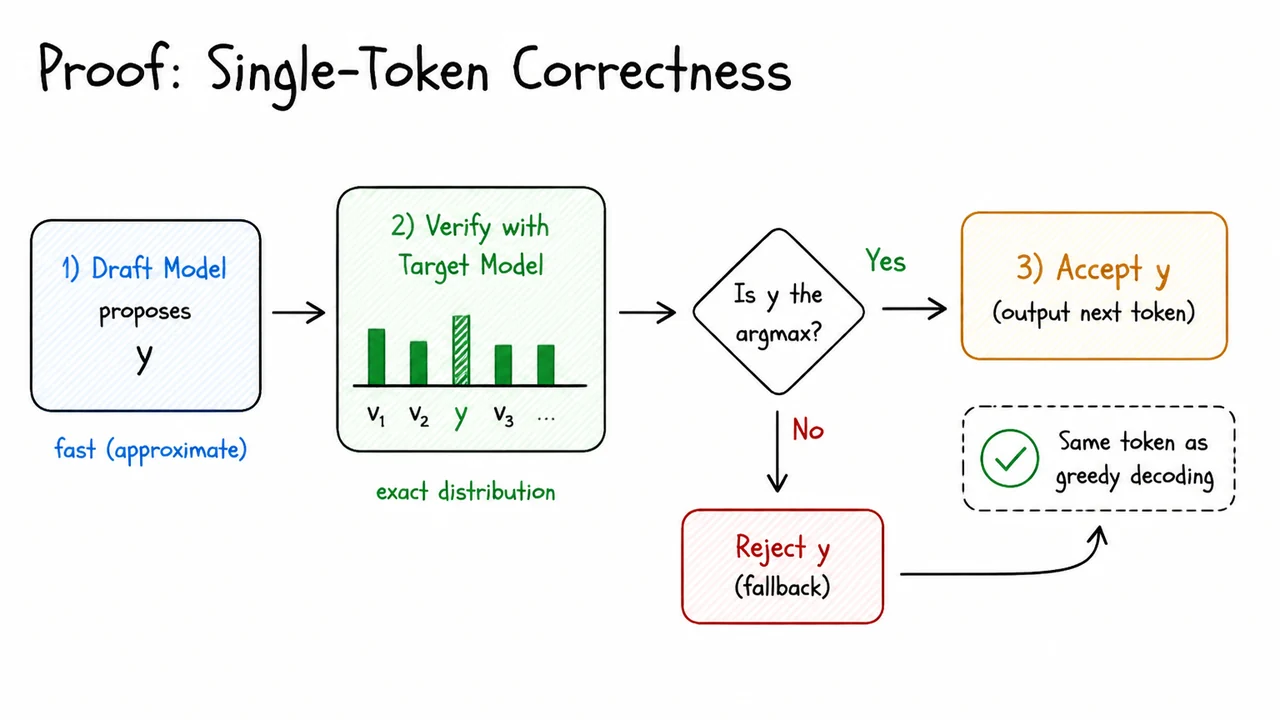
To see why speculative decoding works at all, we must first understand the simplest case: generating a single token. The full algorithm builds on this base step, so proving single‑token correctness is not just a warm‑up – it is the atomic unit that induction will later chain together. The previous section stated the overall correctness theorem; now we prove the base case, showing that when we sample one token from a draft model and then apply a carefully chosen acceptance‑and‑resampling rule, the token we finally output is distributed exactly as if we had run the expensive target model $p$ in the first place.

Consider a large language model $p$ that defines a distribution over a huge vocabulary $\mathcal{V}$. We want to sample a token $x \sim p$. Instead of evaluating $p(x)$ for every $x$ (which requires a full forward pass through the target model), we first sample a candidate token $x$ from a cheaper draft model $q$. The draft model is not identical to $p$ – if it were, we would simply use $q$ – but it often assigns high probability to the same tokens that $p$ favours. The challenge is to correct the discrepancy without ever computing the full $p$ distribution. Rejection sampling offers a classic solution, but it requires a global constant $M \ge \max_x \frac{p(x)}{q(x)}$. In language models with tens of thousands of tokens, finding such an $M$ is impractical, and using a loose bound kills efficiency because the acceptance rate plummets.

Speculative decoding sidesteps this by splitting the correction into two phases: a stochastic acceptance gate and a deterministic residual resampling. Given a token $x$ drawn from $q$, we accept it with probability
$$\alpha(x) = \min\!\left(1,\; \frac{p(x)}{q(x)}\right).$$ If the draft model underestimates the target ($p(x) > q(x)$), we always accept; if it overestimates ($q(x) > p(x)$), we accept with a probability that exactly compensates for the excess. This rule emerges from a simple observation: the quantity $\min(q(x), p(x))$ is the maximum common probability mass the two distributions assign to $x$. When we accept a token, we keep a portion of that shared agreement. When we reject, however, we are left with the probability mass where $q$ overshoots $p$. The total rejection probability is
$$Z = \sum_{x} q(x)\bigl(1 - \alpha(x)\bigr) = \sum_{x} \bigl(q(x) - p(x)\bigr)_+,$$ where $(a)_+ = \max(a,0)$. This $Z$ is exactly the total variation distance component where the draft has greater mass.

Now the crucial step: we must re‑inject the rejected probability in such a way that the overall distribution becomes $p$. The algorithm defines a residual distribution
$$p_{\text{res}}(x) = \frac{\bigl(p(x) - q(x)\bigr)_+}{Z}$$ and, upon rejection, draws a token from $p_{\text{res}}$ instead. Geometrically, this residual captures the tokens where $p$ dominates $q$ – precisely the places we need additional probability to match the target. The denominator $Z$ is not only the rejection probability but also the total amount of missing mass, because
$$\sum_x \bigl(p(x)-q(x)\bigr)_+ = \sum_x \bigl(q(x)-p(x)\bigr)_+ = Z.$$ (This equality follows from $\sum (p-q) = 0$.) So the rejection event acts as a perfect funding mechanism: every rejected draw funds exactly one corrective draw from the residual, with the same total weight $Z$.

We can now compute the final probability of emitting any token $x$. The token can appear either through acceptance from $q$ or through a corrective draw after rejection. The acceptance path contributes $\min(q(x), p(x))$; the corrective path contributes $Z \cdot p_{\text{res}}(x) = (p(x)-q(x))_+$. Adding them together: $$P(\text{output } x) = \min\bigl(q(x),\,p(x)\bigr) + \bigl(p(x)-q(x)\bigr)_+.$$ A case analysis shows this always equals $p(x)$. If $p(x) \le q(x)$, then the minimum gives $p(x)$ and the positive part is zero; if $p(x) > q(x)$, the minimum gives $q(x)$ and the positive part supplies the missing $p(x)-q(x)$. In either case, the sum collapses to $p(x)$. Thus, the single‑step process is lossless: the output token is distributed identically to a token sampled directly from the target model.

The visual below distills this argument into a compact diagrammatic proof. A single token starts with a sample from the draft distribution $q$. It passes through an acceptance gate that flips a coin with bias $\min(1, p/q)$. The accepted branch goes straight to the output; the rejected branch triggers a resample from the residual distribution. The annotated flows of probability mass at each split make it immediate that, token by token, the total probability of reaching any $x$ is exactly $p(x)$. This sketch not only reinforces the algebraic derivation but also reveals why the scheme extends naturally to longer sequences: the same correction principle applies at each step, and a formal induction will take care of the rest.

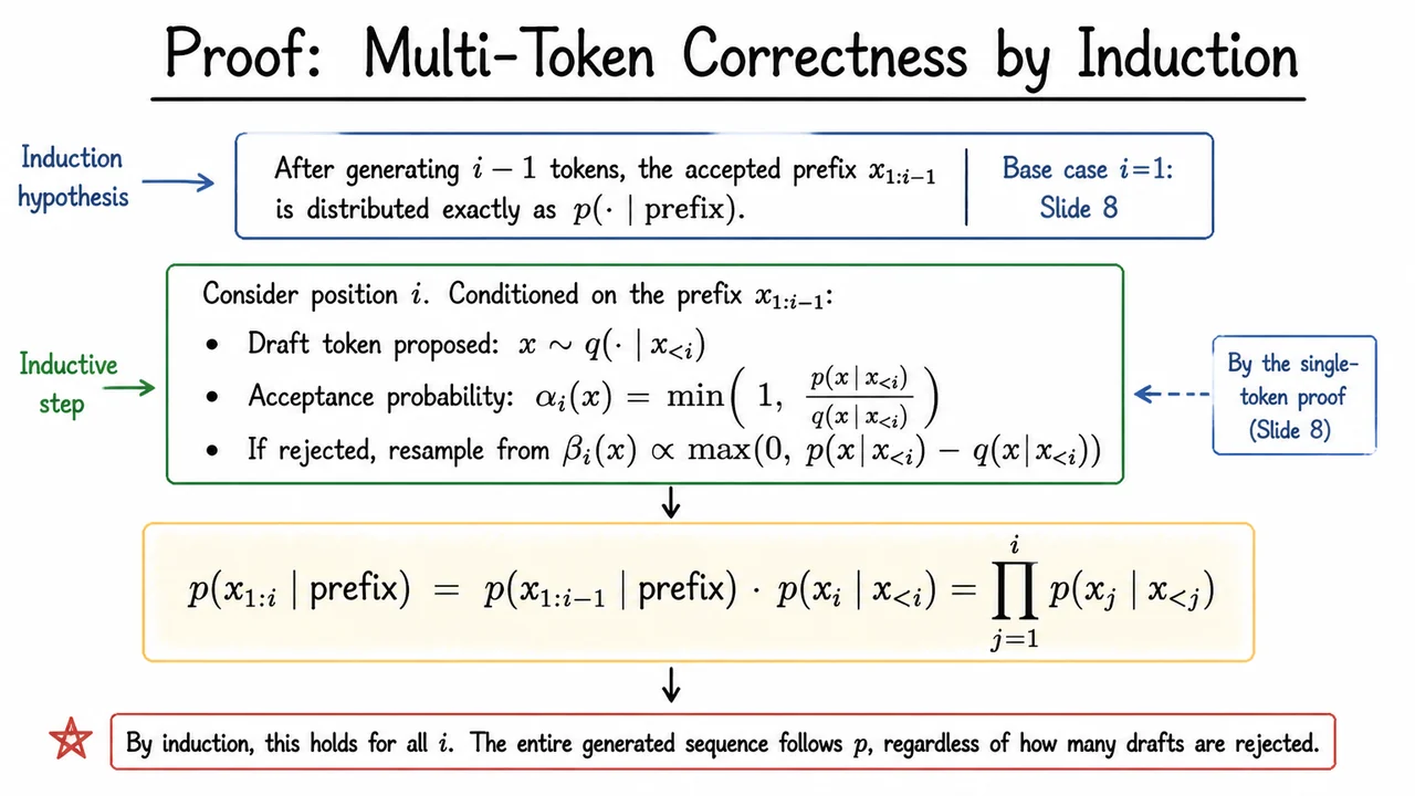
The previous section established that, for a single position, the speculative decoding procedure draws a token exactly from the target distribution $p(\cdot \mid x_{<i})$. That one-step guarantee is a triumph of rejection sampling, but it says nothing about the sequence as a whole. If we simply run that step over and over, do the dependencies between positions accumulate some hidden bias? The answer—perhaps surprisingly—is no. By a simple induction argument, the entire generated prefix at every step remains distributed according to the target model $p$. The result is dramatic: speculative decoding is lossless in the strict probabilistic sense, regardless of how cheap the draft model $q$ may be or how many tokens are accepted or rejected.

To appreciate the induction, it helps to step back and ask what it means for a prefix to be “correctly distributed.” In autoregressive generation, the probability of a token is always conditioned on all prior tokens. So if we have a prefix $x_{1:i-1}$ that is truly a random sample from $p(\cdot \mid \text{prefix})$—meaning the joint probability of that prefix matches what the target model would produce—then any token added according to the correct conditional $p(x_i \mid x_{<i})$ will keep the longer prefix faithful to $p$. The induction simply formalizes this intuition: the base case is the given prefix (empty or user-supplied), and each subsequent token is drawn from the right conditional because of the single-token proof. No unseen correlations can sneak in, because the Markovian nature of the target model ensures that all future randomness is conditionally independent of the past given the current prefix.

The induction hypothesis is then straightforward. For any integer $i \ge 1$, assume that after $(i-1)$ tokens are accepted, the sequence $x_{1:i-1}$ is distributed exactly as $p(\cdot \mid \text{prefix})$. When $i=1$, this is the empty prefix, which trivially satisfies the hypothesis; that base case was checked in the single-token proof. Now for the inductive step at position $i$: conditioned on the prefix $x_{1:i-1}$, the speculative decoding algorithm takes three actions. First, it proposes a draft token $x \sim q(\cdot \mid x_{<i})$. Then it computes the acceptance probability

$$\alpha_i(x) = \min\!\bigl(1,\; \frac{p(x\mid x_{<i})}{q(x\mid x_{<i})}\bigr).$$

If rejected, the algorithm does not simply discard the token and stall; it resamples a replacement from the residual distribution

$$\beta_i(x) \propto \max\bigl(0,\; p(x\mid x_{<i}) - q(x\mid x_{<i})\bigr).$$

The single-token proof—already established—shows that regardless of the draft model $q$, the token that finally lands at position $i$ follows exactly $p(\cdot \mid x_{<i})$. In other words, the marginal distribution of the added token is the target conditional, even though the acceptance mechanism uses $q$ to propose.

Now we can chain these conditionals. The joint probability of the new extended prefix $x_{1:i}$ given the original prompt is

$$p(x_{1:i} \mid \text{prefix}) = p(x_{1:i-1} \mid \text{prefix}) \cdot p(x_i \mid x_{<i}),$$

by the definition of autoregressive factorization. The induction hypothesis tells us that the first factor is exactly the product we want for positions $1$ through $i-1$, while the single-token proof guarantees the second factor is the correct conditional for position $i$. Multiplying them gives the product over all $i$ positions:

$$p(x_{1:i} \mid \text{prefix}) = \prod_{j=1}^{i} p(x_j \mid x_{<j}).$$

Therefore the extended prefix follows the target distribution. By induction, this holds for every $i$, no matter how many tokens are generated. A few subtle points deserve attention. The acceptance and resampling decisions at each step depend on $q$ and on random bits, but these sources of randomness are all independent across steps conditionally on the prefix. Thus the induction does not require any special independence beyond what the target model itself encodes. Moreover, the length of the generated sequence is determined by stopping conditions (e.g., end-of-sequence token or max length); the induction still applies because each accepted token in the prefix is from $p$ regardless of when the process stops.

This multi‑token correctness is the backbone of speculative decoding’s losslessness claim. It means that no matter how aggressively we draft tokens with a cheap model, and no matter how many of those drafts are rejected, the output sequence is statistically indistinguishable from one produced by running the expensive target model one token at a time. The speed gains come from the fact that we often accept several tokens in a row, processing them in parallel, but we never pay a probability-of-error cost.

The visual below captures this proof in a compact, digestible form. It opens with the induction hypothesis box, reminding us that the prefix up to $i-1$ already follows $p$. An indented block then presents the inductive step: the three bullet points for draft proposal, acceptance, and resampling, each with its defining expression. These are deliberately kept sparse so that the reader sees the logical flow rather than dense algebra. At the center, the key factorization equation appears prominently on a light background—$p(x_{1:i} \mid \text{prefix}) = \prod_{j=1}^{i} p(x_j \mid x_{<j})$—which is exactly the conclusion of the inductive step. Arrows and brackets link the single‑token guarantee to the overall joint distribution, and a final sentence reassures that by induction the whole sequence belongs to $p$. The color accents (blue for references, muted tones for the hypothesis and conclusion) guide the eye without distraction, turning what could be a dense slide of equations into a clear conceptual map of the proof.

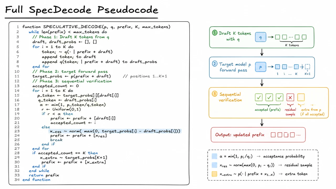
Having established that the multi‑token acceptance procedure preserves the exact target distribution, we are ready to assemble the complete speculative decoding loop. The algorithm operates as a while‑loop that repeatedly drafts, scores, and verifies tokens until the desired sequence length is reached. It is deceptively simple, yet each detail—from how the draft is produced to how a rejection is handled—is precisely calibrated to guarantee that every token emitted by the combined system follows the large model’s distribution $p$.

The outer structure is a loop that runs while the current prefix is shorter than max_tokens. In every iteration we aim to add up to $K+1$ tokens, where $K$ is a hyperparameter that trades off the draft model’s speed against the verification cost. The first step, Phase 1, generates a draft of length $K$ from the small draft model $q$. Because $q$ is cheap to run, we can afford to sample autoregressively: starting from the current prefix, we draw token $x_1 \sim q(\cdot \mid \text{prefix})$, then $x_2 \sim q(\cdot \mid \text{prefix} + x_1)$, and so on. At each step we record both the sampled token and its probability under $q$. The result is a list of $K$ tokens—the draft—and a parallel list of their $q$‑probabilities, which we will need for the acceptance test.

Phase 2 then brings in the large target model $p$. Because $p$ is expensive to call, we want to amortise its cost over many tokens. The trick is to feed the entire concatenated sequence prefix + draft into $p$ in a single forward pass. Since the draft has length $K$, the model can compute logits (and hence probabilities) for the positions after the prefix, i.e. for draft positions $1$ through $K$ as well as for position $K+1$, which corresponds to the token that would follow the full draft. This provides us with $K+1$ probability vectors: for each $i \in \{1,\dots,K\}$, target_probs[i] is the distribution $p(\cdot \mid \text{prefix} + x_{1..i-1})$, and target_probs[K+1] is $p(\cdot \mid \text{prefix} + x_{1..K})$. Notice how this parallel probing completely avoids the sequential bottleneck of drawing one token at a time from $p$.

With both the draft probabilities and the target probabilities in hand, Phase 3 performs a sequential verification that mirrors the rejection‑sampling logic we proved correct earlier. The loop walks through the draft positions from $i=1$ to $K$. For the $i$-th draft token $x_i$, we retrieve its probability under $p$ and under $q$. The acceptance probability is the familiar min‑ratio:

$$\alpha_i = \min\!\left(1, \frac{p(x_i \mid \text{prefix} + x_{1..i-1})}{q(x_i \mid \text{prefix} + x_{1..i-1})}\right).$$

We draw a uniform random number $r \in (0,1)$ and accept $x_i$ if $r < \alpha_i$. Upon acceptance we append the token to the prefix, record the accepted count, and proceed to examine $x_{i+1}$. If we reject the token, we do not simply discard it; we replace it with a correction drawn from the residual distribution

$$\beta_i(x) \propto \max\!\bigl(0,\; p(x \mid \text{prefix} + x_{1..i-1}) - q(x \mid \text{prefix} + x_{1..i-1})\bigr),$$

append that correction, and then break out of the verification loop. This correction step is essential: it guarantees that, despite the draft model’s bias, the final token that appears at position $i$ is distributed exactly as if we had sampled from $p$ directly.

After the verification loop, if we managed to accept all $K$ draft tokens (i.e., accepted_count == K), we are allowed to sample one additional token from the already‑computed target_probs[K+1]. This “bonus” token exploits the extra forward‑pass information and brings the maximum possible tokens per iteration to $K+1$. The updated prefix now contains the original prefix, the accepted (and possibly one corrected) draft tokens, and sometimes the bonus token, and the outer loop continues.

The entire procedure interleaves draft generation and rigorous distribution‑matching verification in a seamless while‑loop. Because the acceptance criterion, the residual resampling, and the bonus‑token rule are derived directly from rejection‑sampling principles, the output remains losslessly aligned with the target model—no approximation is introduced. In the next section we will analyse how many tokens we should expect to generate per iteration, but for now the algorithm itself is the object of study.

The visual below condenses this algorithm into a clean pseudocode reference. It places the three‑phase structure in a bordered box, uses a monospaced font for readability, and lightly highlights the critical acceptance and residual‑sampling lines. This layout lets you absorb the interplay between draft, forward pass, verification, and the corrective sampling at a glance, while reserving the detailed reasoning for the surrounding prose.

Building on the full SpecDecode pseudocode, we now need a way to measure what the algorithm actually pays off in practice. The core idea is that an iteration checks a batch of $K$ draft tokens produced by the cheap model $q$ and accepts each with probability $\min\!\bigl(1, p(x)/q(x)\bigr)$. The process stops as soon as a token is rejected—at that point the target model’s corrected residual token takes over. So the number of tokens we can generate in a single iteration is precisely the length of the accepted prefix, plus that one residual token. Understanding this count is the key to quantifying speed‑ups and to knowing when speculative decoding actually works.

We begin by defining the per‑token acceptance probability. Under the draft distribution $q$, the chance that a proposed token $x$ survives the verification step is $\min\!\bigl(1,\frac{p(x)}{q(x)}\bigr)$. Averaging over the draft model’s own outputs gives the expected acceptance probability, a single scalar that captures how well the two models agree:

$$\alpha \;=\; \mathbb{E}_{x\sim q}\!\Bigl[\min\!\bigl(1,\,\frac{p(x)}{q(x)}\bigr)\Bigr] \;=\; \sum_{x\in V} q(x)\,\min\!\bigl(1,\frac{p(x)}{q(x)}\bigr).$$

It is easy to miss how neatly $\alpha$ links to a classical measure of distributional distance. Observe that

$$\sum_x q(x)\min\!\bigl(1,\frac{p(x)}{q(x)}\bigr) = \sum_x \min\!\bigl(q(x), p(x)\bigr),$$

because multiplying the minimum by $q(x)$ inside the sum selects the smaller of the two probabilities pointwise. Now the total variation distance (TVD) between $p$ and $q$ is defined as

$$\operatorname{TVD}(p,q) = \frac12\sum_x |p(x)-q(x)|,$$

and it is a standard exercise to show that $\sum_x \min(q,p) = 1 - \operatorname{TVD}(p,q)$. Indeed, the total probability mass where $q$ exceeds $p$ is exactly $\operatorname{TVD}(p,q)$, and subtracting that from 1 leaves the overlapping mass. Hence

$$\boxed{\alpha = 1 - \operatorname{TVD}(p,q)}.$$

This identity is the first crucial insight: the expected acceptance probability drops linearly with the total variational distance between the draft and target distributions. When the two models are identical, $\operatorname{TVD}=0$ and $\alpha=1$; every draft token is accepted. As the distributions pull apart, $\alpha$ declines, and the expected number of consecutive acceptances falls sharply.

With $\alpha$ in hand we can model the acceptance process across the $K$ draft positions. Because the probability of accepting a token given the current state depends only on the local distributions $p$ and $q$, we can treat the decisions as independent Bernoulli trials, each with success probability $\alpha$, for the purpose of an aggregated expectation (the actual process is of course conditional, but under stationarity assumptions the marginal probability of a string of $n$ acceptances behaves like $\alpha^n$). The number of consecutive accepted draft tokens before the first rejection—or before we simply run out of draft tokens—is then a truncated geometric random variable $N$ with

$$\Pr(N \ge n) = \alpha^{\,n}, \qquad n = 0,1,\dots,K.$$

From this we can compute the expected number of accepted draft tokens per iteration:

$$\mathbb{E}[N] = \sum_{n=1}^{K} \alpha^{\,n} = \alpha\,\frac{1-\alpha^{K}}{1-\alpha}.$$

But the iteration actually produces one more token: either the corrected token from the residual resampling step (when $N < K$) or an extra token sampled directly from the target distribution $p$ after all $K$ draft positions have been accepted. Thus the expected number of newly generated tokens per speculative iteration is

$$\boxed{\mathbb{E}[\text{tokens added}] = \mathbb{E}[N] + 1 = \frac{1-\alpha^{K+1}}{1-\alpha}}.$$

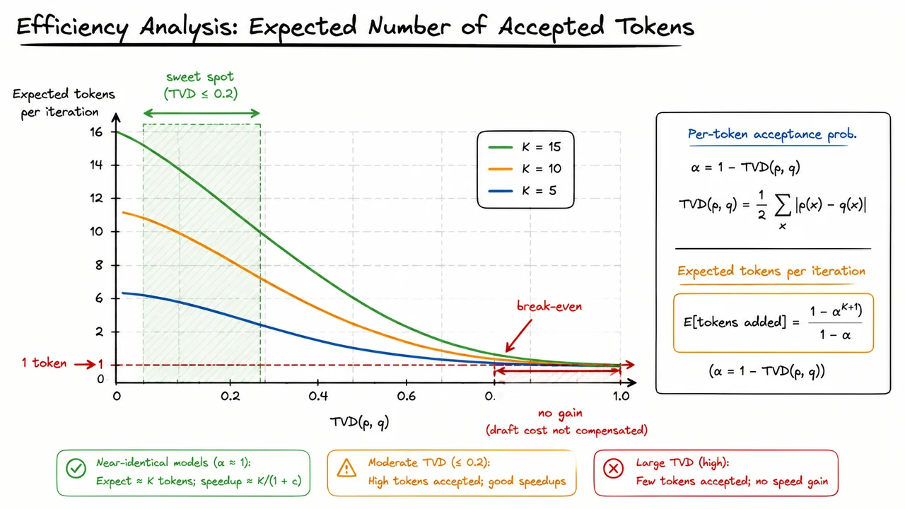
When the models perfectly match ($\alpha = 1$), the limit of this expression is $K+1$ — exactly the full speculative window plus one final token. When disagreement grows ($\alpha \to 0$), the series approaches 1, meaning we only obtain a single token per iteration and the draft model contributes nothing but overhead.

The practical benefit of this formula is that it puts a number on what an implementer really cares about: inference speed‑up. Let the target model cost one unit of time per token in the normal autoregressive loop, and let the draft model cost $c$ units per token (with $c \ll 1$). A speculative iteration costs roughly the target’s parallel forward pass for $K+1$ tokens (whose cost is similar to generating one token, up to a constant factor) plus the draft’s forward passes for $K$ tokens. If we approximate the target’s parallel pass as one unit, the per‑iteration cost is $1 + cK$. The effective speed‑up over standard decoding is then proportional to

$$\frac{\mathbb{E}[\text{tokens added}]}{1 + cK} \approx \frac{(1-\alpha^{K+1})/(1-\alpha)}{1 + cK}.$$

This expression makes plain the tension between draft length, draft accuracy, and cost. When $\alpha$ is very high—say $\operatorname{TVD}$ is below $0.1$—almost all $K$ draft tokens are accepted, and the speed‑up approaches $K/(1+cK)$. In that regime, picking a longer speculation window can yield dramatic gains. Conversely, if $\operatorname{TVD}$ exceeds roughly $0.3$ to $0.5$, $\alpha$ drops quickly and the expected tokens collapse toward $1$; the cost of the draft model dominates and the speed‑up disappears or even becomes a slow‑down.

The visual below turns this analysis into a clear decision aid. It plots the expected number of tokens per iteration against $\operatorname{TVD}(p,q)$ for several values of the speculation length $K$ (e.g. 5, 10, 15). Each curve starts at $K+1$ when the models are identical ($\operatorname{TVD}=0$) and decays rapidly as TVD grows. The plot highlights a “sweet spot” where the draft model is accurate enough ($\operatorname{TVD} \lesssim 0.2$) that expected tokens remain close to $K+1$, resulting in substantial acceleration. A “break‑even” region shows where the gain shrinks down to roughly 1 token per iteration, and a “no‑gain” zone warns where the draft model’s overhead cannot be recouped. The annotation of these zones directly connects the abstract $\alpha$ formula to the engineering reality: speculative decoding only provides a practical speed‑up when the draft model and target model are strongly aligned. For a practitioner, the plot is an immediate diagnostic: before deploying, one should measure TVD on representative prompts and choose a speculation length that sits comfortably within the sweet spot.

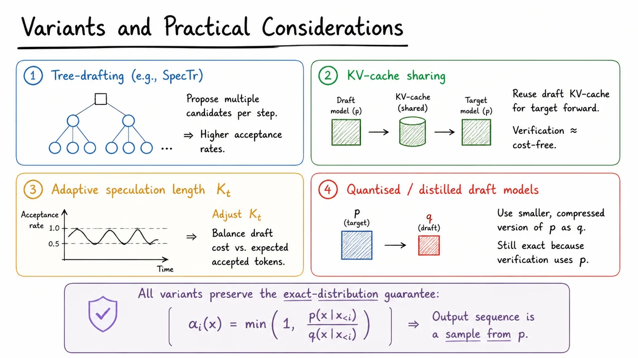
Having analyzed the expected number of tokens that speculative decoding will accept under ideal conditions, we can now examine a set of practical enhancements that make the method faster and more robust without ever sacrificing its central guarantee: that the output distribution remains exactly that of the target model $p$. The theoretical efficiency analysis revealed that the acceptance rate depends on the closeness of the draft model $q$ to $p$, but it left open questions about how to improve the effective throughput when drafting costs are non‑negligible, when the optimal lookahead depth varies with context, or when we want to deploy the technique under tight memory budgets. The variants discussed here answer these questions by cleverly reusing computation, dynamically adjusting the speculation length, broadening the verification step to cover multiple parallel proposals, and trading off draft model quality against resource footprint. All of them preserve the exactness of the sampling procedure because they leave the acceptance criterion unchanged.

Tree‑drafting generalizes the linear chain of speculative tokens to a tree of candidate continuations. Instead of proposing a single next token and then conditionally proposing the token after that, a faster draft mechanism can generate several alternative first tokens in parallel, followed by branches that extend each of those possibilities. The target model then scores the entire tree in one forward pass, using a block‑diagonal attention mask that respects the branching structure. The verification step becomes a top‑down process: starting from the root, we examine the children, accept one with probability $\min(1, p/q)$ for that branch, and then descend into the corresponding subtree, repeating the acceptance test at each level. This increases the chance of accepting a long prefix because multiple candidate prefixes compete simultaneously. However, a subtle failure mode is that an overly wide or deep tree can inflate the cost of the target forward pass without a commensurate gain in acceptance length; careful pruning of the draft tree, often based on the local $q$ probabilities, is required. The advantage is purely practical: tree‑drafting reduces the number of target calls per generated token without relaxing the exactness condition, because the rejection‑sampling logic is applied independently to each edge in the tree.

KV‑cache sharing tackles the latency of the verification forward pass. If the draft model and the target model share an identical tokenizer and a compatible attention architecture—for example, when the draft is a pruned, quantized, or early‑exit version of the target—the key‑value pairs computed during the draft phase can be reused for the target’s attention layers. The target model can skip recomputing the representations for all the tokens that the draft already processed, and only needs to attend to the newly proposed tokens. This makes the verification step nearly cost‑free in terms of computation, effectively decoupling the verification latency from the target model’s size. The primary requirement is architectural compatibility; a mismatch in hidden dimensions or head counts would break the reuse. When the draft is a heavily compressed variant of $p$, cache sharing turns a speculative step into a tiny draft forward pass plus a cheap “re‑scoring” of the proposals using the cached states.

Adaptive speculation length $K_t$ addresses the fact that a static number of speculative tokens is rarely optimal. The expected number of accepted tokens depends on the local divergence between $p$ and $q$, which can vary across contexts: for highly predictable text, many tokens might be accepted in a row, while in a surprising passage the acceptance rate drops and long speculative chains waste draft compute. By tracking recent acceptance statistics, the system can adjust $K_t$ dynamically—growing $K$ when recent acceptance rates are high and shrinking it when they are low. This dynamic schedule can be as simple as a moving average with a threshold, or it can use a more sophisticated controller that optimizes an estimate of tokens‑per‑second. Crucially, changing $K_t$ does not affect the per‑token acceptance probability $\alpha_i$; it only determines how many tokens we try to generate before we stop and call the target model for verification. The exactness guarantee is untouched because each speculative step still applies the same rejection sampling rule, and the eventual token sequence is drawn from $p$ irrespective of where we stop the chain.

Quantized or distilled draft models push the resource argument further. By aggressively quantizing the draft model’s weights or distilling it from the target distribution, we can obtain a $q$ that is orders of magnitude faster to run than the full‑precision, large target, yet still retains a meaningful acceptance rate. Because the verification step always uses the true $p$ to compute $\alpha_i$, any mismatch in the draft’s quality is automatically corrected—the output remains a perfect sample from $p$. The only penalty is a lower acceptance rate, but the dramatic reduction in draft cost often more than compensates. In the extreme, one can even use a simple n‑gram model or a lightweight rule‑based proposal as $q$; as long as we faithfully compute $\min(1, p/q)$ and perform the residual resampling when a token is rejected, the sequence is guaranteed to be from $p$. This opens the door to running speculative decoding on devices where even a small transformer draft is too heavy, or to pairing a state‑of‑the‑art target model with a fast draft trained on a different corpus.

All these variants share a common theoretical backbone: the acceptance probability $$\alpha_i(x) = \min\!\left(1, \frac{p(x\mid x_{<i})}{q(x\mid x_{<i})}\right).$$ This single equation encodes the rejection‑sampling step that makes the overall procedure a lossless accelerator. Whether we are verifying a flat sequence, traversing a tree, or reusing caches, the decision at each position $i$ is computed using the draft probability $q$ that was used to propose the token and the target probability $p$ of that same token under the correct language model. The resulting token distribution is exactly $p$, and the only thing that changes from variant to variant is how the proposals are generated and how expensive it is to evaluate $p$ and $q$. The exactness guarantee is therefore robust: any proposal distribution that satisfies the standard condition of being absolutely continuous with respect to $p$ can be plugged into the same verification logic.

The visual below distills these insights into a compact reference. It arranges the four principal variants—tree‑drafting, KV‑cache sharing, adaptive $K_t$, and quantized/distilled draft models—into a 2×2 grid, each with a brief, large‑print label that captures its core idea. At the bottom, a centered equation box displays the universal acceptance criterion, making it immediately clear that all paths converge to the same rejection‑sampling step. This diagram serves as a quick mental map: when you need to engineer a lossless acceleration pipeline, you can mix and match these techniques knowing that the output distribution will stay exactly $p$ as long as the verification step respects that one equation.

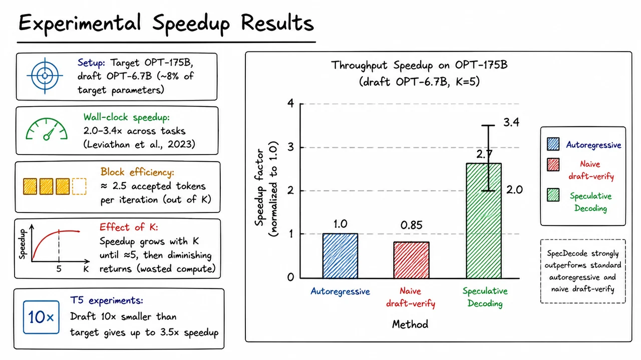
After exploring the algorithmic variants and practical engineering choices that make speculative decoding viable, we turn to the question that matters most in deployment: how much faster does it actually run? Theoretical guarantees of losslessness are comforting, but they say nothing about wall‑clock latency. The original paper by Leviathan et al. (2023) provides a careful empirical picture, and the numbers are encouraging — speculative decoding consistently delivers a 2 – 3.5× speedup over standard autoregressive generation for large Transformer models, without altering the output distribution by even a single token.

The headline experiments pair OPT‑175B as the target model with OPT‑6.7B as the draft model. The draft has only about 8 % of the target’s parameter count, so running it forward $K$ times is cheap relative to one forward pass of the 175 B giant. The tasks span dialogue, summarisation, and translation — distinct enough to ensure the results are not an artefact of a single data domain. Across these settings, the measured wall‑clock speedup ranges from 2.0× to 3.4×. Wall‑clock timing is critical because it accounts for all overhead: draft model execution, target model verification, the cost of the modified rejection‑sampling logic, and any I/O or synchronisation. A 3× end‑to‑end acceleration means a 175B model responds in one third of the time, transforming an interactive chat assistant from barely tolerable to fluid.

A complementary metric is block efficiency, defined as the average number of accepted tokens per speculation iteration. With a speculation length $K = 5$, the observed block efficiency sits around 2.5 accepted tokens per iteration. In other words, about half the draft tokens pass the acceptance test. This fraction is not a sign of a weak draft — it’s actually the sweet spot. If the draft were so good that it predicts nearly every token correctly, we would be better off simply using the draft as the target; if it predicts too few, the overhead of running the draft becomes uneconomical. The 2.5‑token average means that each verification pass of the large model buys us more than two tokens of progress, amortising its enormous cost.

The choice of $K$ strongly influences the speedup, and the empirical curve reveals a classic diminishing‑returns pattern. As $K$ increases, the target model verifies longer speculative sequences, so if many tokens are accepted, we commit more generation steps at once. Beyond $K \approx 5$, however, the benefit plateaus or even degrades. The reason is simple: longer drafts tend to drift further from the target distribution, raising the probability of a rejection that discards not only the offending token but all subsequent draft tokens. Those rejected tokens represent wasted computation in the draft model. Finding the optimal $K$ is therefore a balancing act between ambition and discipline, and the experiments show that $K$ in the range 3–6 is broadly effective for draft models of this scale.

The phenomenon is not specific to the OPT family. Experiments with T5 models confirm the same behaviour: when the draft is an order of magnitude smaller than the target (roughly 10 % of parameters), speculative decoding achieves up to 3.5× speedup. This robustness across architectures suggests that as long as the draft model’s output distribution resembles that of the target — a condition met by any reasonably well‑trained smaller variant or a model from the same family — the acceleration is substantial.

It is instructive to compare speculative decoding against a straw‑man baseline: naive draft‑then‑verify. In that approach, one simply runs the draft model to generate $K$ tokens, then asks the target model to evaluate that sequence without any correction or resampling. The problem is that even a few wrongly predicted tokens can accumulate, producing text that diverges from the target distribution and often requires expensive correction or premature termination of generation. Empirically, naive draft‑then‑verify actually slows down generation (about 0.85× the speed of plain autoregressive decoding) because the overhead of running the draft and then having the target model process a low‑quality sequence outweighs any possible gain.

The visual below makes these comparisons concrete. It shows a bar chart of throughput speedup on the OPT‑175B setup with $K=5$. The Autoregressive bar sits at 1.0, the natural baseline. The Naive draft‑verify bar falls noticeably below 1.0, vividly illustrating that simply chaining a draft with a verifier without the rejection‑sampling step is counter‑productive. The Speculative Decoding bar rises to a central value of 2.7×, accompanied by error bars that mark the 2.0–3.4× range observed across tasks. The chart title — Throughput Speedup on OPT-175B (draft OPT-6.7B, K=5) — anchors the precise experimental condition. The contrast between the three bars does not merely report numbers; it tells a story: lossless acceleration is achievable, but only when verification is followed by the careful probabilistic rejection and resampling that preserves the target distribution. This single image encapsulates why speculative decoding is not a gimmick but a principled leap forward in efficient LLM inference.

After seeing the raw speedup numbers, the natural next question is why some settings show dramatic wall‑clock improvements while others barely budge—or even regress. Speculative decoding is not a universal accelerator; its effectiveness pivots on a handful of interacting factors that are easy to miss when the method is presented only as a clever rejection‑sampling trick. Unpacking those factors transforms the empirical results into a predictive mental model, which is exactly what this section aims to build.

The core trade‑off is between the quality of the draft model and the cost ratio of the two models. Let the draft model’s per‑step cost be $c_d$ and the target model’s cost be $c_t$. A single speculative step runs the draft for $k$ tokens (cost $k c_d$) and the target for one parallel verification pass (cost $c_t$). If the draft’s proposals are accepted with probability $\alpha$ on average, each verified step produces $1 + \alpha(k-1)$ tokens in expectation, because the first token is always kept and each subsequent token has an independent $\alpha$ chance of acceptance. The expected speedup over running the target alone is therefore

$$S = \frac{1 + \alpha(k-1)}{c_t} \Big/ \frac{1}{c_t + k c_d} \approx \frac{1 + \alpha(k-1)}{1 + k\,(c_d/c_t)}.$$

This expression already illuminates the first major condition: $\alpha$ must be high enough to overcome the extra draft compute. If the draft is a small, fast model ($c_d / c_t \ll 1$), even moderate $\alpha$ can yield gains. But if the draft is too expensive or too often wrong, the numerator grows slower than the denominator, and speculative decoding can become slower than just using the target.

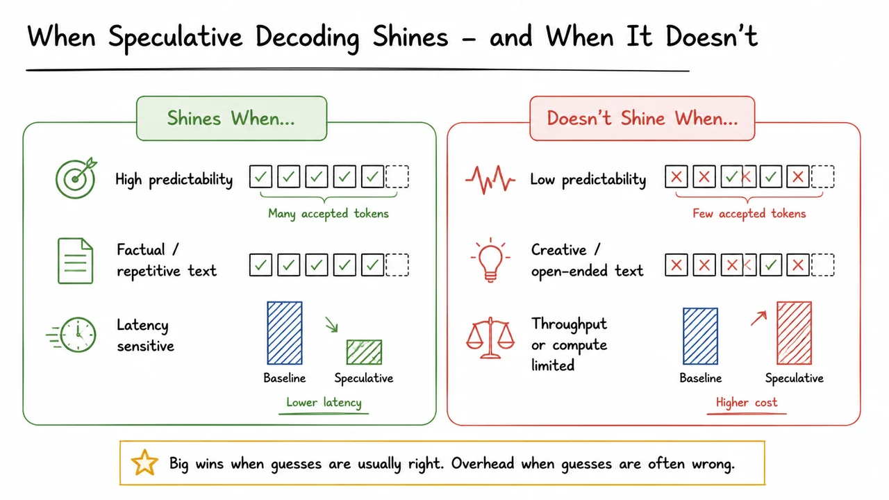
The acceptance probability $\alpha$ itself is not a fixed property. It depends on the divergence between the draft and target distributions, and critically on the temperature used during generation. At high temperatures, the target’s distribution flattens, so the chance that the draft’s greedy (or sampled) token matches the target’s highest‑probability token drops. This leads to low acceptance and many wasted draft tokens. Conversely, low‑temperature, fact‑based, or formulaic generation (e.g., code completion, summarization) produces tight distributional consensus between a decent draft and the target, pushing $\alpha$ close to 1. Empirical studies repeatedly confirm that speculative decoding shines on deterministic or low‑entropy text, and its speedup erodes for open‑ended creative writing.

A second critical factor is generation length. Speculative decoding amortizes the fixed overhead of loading and running the target model over multiple tokens per verification step. For very short responses—say, one‑shot classification or a 5‑token answer—the startup cost dominates, and the method may never break even. The largest speedups materialize in long, coherent continuations where each verification pass reliably adds a block of new tokens.

Domain alignment between draft and target further magnifies (or destroys) $\alpha$. A general‑purpose draft, e.g., a small Llama model, can mimic a larger Llama target across many genres because they share pretraining data and tokenization. Replace the pair with mismatched architectures, vocabularies, or training corpora (like using a code‑specialized draft for a medical target), and $\alpha$ plummets. Fine‑tuning the draft on the target’s output distribution is often a high‑return engineering investment.

Other practical constraints matter, too. Batch size: speculative decoding is a per‑sequence method; verifying multiple sequences in parallel shares the target forward pass but forces the draft to run independently for each sequence. In large batch regimes, throughput rather than latency is the metric, and the extra draft compute may reduce overall throughput if GPUs are already saturated. Hardware memory also plays a role—the target model may already fill the accelerator, leaving no room for the draft, which pressures system design.

The visual that accompanies this section distills these insights into a pair of contrasting scenarios. On one side, a high‑alignment, low‑temperature setting (e.g., code completion) shows a large forward leap with many accepted tokens in a single verification step, labelled with “strong draft alignment”, “low entropy”, “long generation”. On the other, a high‑temperature, creative‑writing setting shows a draft that repeatedly proposes tokens that get rejected, resulting in short leaps and wasted compute, labelled with “poor draft match”, “high temperature”, “short output”. Together, they form a quick mental checklist: before adding speculative decoding to a production system, first ask how well the draft anticipates the target and how much entropy the task expects to see.

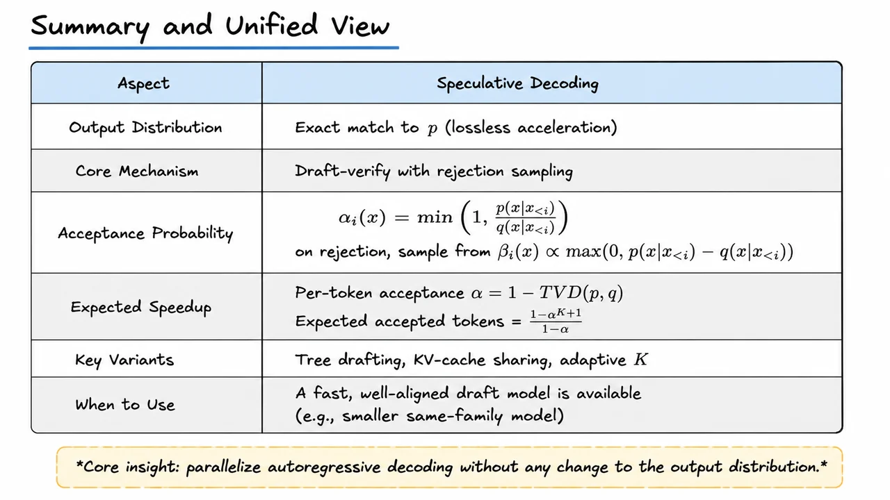
As we step back from the specific regimes where speculative decoding excels or falls short, a unified picture emerges—one that is both mathematically elegant and practically transformative. At its heart, speculative decoding guarantees lossless acceleration: the sequence of tokens generated by the system is exactly that which would be produced by the large target model in its normal autoregressive loop, yet the wall‑clock time can be cut to a third or half. This dual promise of exact distributional fidelity and substantial speedup is what makes the technique so compelling; it does not trade off output quality for faster generation, nor does it require re‑training the target model. Understanding how this is achieved and what parameters govern the efficiency brings together all the threads of the lecture.

The bottleneck that speculative decoding overcomes is the fundamentally sequential nature of standard autoregressive decoding, where each token must be sampled before the next can be inferred. Naive attempts to parallelize by sampling multiple tokens independently—perhaps using a large batch of future contexts that ignore the inter‑token dependencies—are doomed to produce a different, uncontrolled distribution. Speculative decoding circumvents this through a draft‑verify loop that speculates on several future tokens at once using a fast approximation, then rigorously corrects the sequence back to the exact target distribution. The verification step leverages principles from rejection sampling, ensuring that every token that survives the process, and those that are re‑sampled after a rejection, are distributed precisely according to $p$.

The core mechanism can be summarized concisely. A small draft model $q$ quickly proposes a block of $K$ candidate tokens $x_1, \dots, x_K$. The large target model $p$ then evaluates this entire block in a single forward pass, obtaining for each position the probability vectors $p(\cdot \mid \text{prefix})$ and $q(\cdot \mid \text{prefix})$. For each candidate token $x_i$, it computes an acceptance probability

$$\alpha_i(x_i) = \min\!\left(1, \frac{p(x_i \mid x_{<i})}{q(x_i \mid x_{<i})}\right),$$

and accepts the token with that probability. If a token is rejected, the system immediately discards all subsequent candidates and samples a corrected token from the residual distribution

$$\beta_i(x) \propto \max\!\bigl(0, \; p(x \mid x_{<i}) - q(x \mid x_{<i})\bigr),$$

before falling back to ordinary autoregressive sampling from $p$. This simple procedure is a proper rejection‑sampling step that transforms the uncorrected draft distribution $q$ into the desired target $p$ one token at a time, and it provably guarantees that the entire generated sequence follows the exact probability law of the target model—the acceleration is lossless.

Why does this work? View it through the lens of single‑token rejection sampling: to sample from $p$ given a proposal $q$, we can accept a candidate $x \sim q$ with probability $\min(1, p(x)/q(x))$, and on rejection, draw from the normalized positive difference $\max(0, p - q)$. This classic trick yields a sample from $p$. In the sequential setting, the same principle applies iteratively: we greedily accept tokens from the draft until a rejection occurs, then sample from the corrected distribution for that position and continue normally. The resulting dependency structure exactly reproduces the target model’s joint distribution. The derivation earlier in the lecture shows that the overall acceptance pattern is equivalent to running a rejection‑sampler that “wraps” the draft block, and the unconditional distribution of the accepted prefix plus the first corrected token matches $p$ for the corresponding prefix length.

The expected speedup captured by the summary table rests on a few clean relationships. The per‑token probability that a draft token is accepted, averaged over the target distribution, is

$$\alpha = 1 - \operatorname{TVD}(p, q),$$

where the total variation distance $\operatorname{TVD}(p,q) = \frac{1}{2}\sum_x |p(x) - q(x)|$ measures the mismatch between the two distributions. In the common case where the draft model is a smaller member of the same family—e.g., a Llama-7B paired with Llama-70B—$\alpha$ can be well above 0.8. Given a block of $K$ draft tokens, the expected number of accepted tokens per block then follows a truncated geometric progression:

$$\mathbb{E}[\text{accepted tokens}] = \frac{1-\alpha^{K+1}}{1-\alpha}.$$

This formula reveals the two knobs that control speedup: the quality of the draft (via $\alpha$) and the length of the draft block $K$. When $\alpha$ is high, the acceptance count approaches $K$ linearly; when $\alpha$ is moderate, the function saturates, meaning that simply increasing $K$ beyond a certain point brings diminishing returns. Together with the cost ratio of the draft model to the target model, these equations allow precise prediction of the overall wall‑clock speedup in practice.

Key variants refine the basic scheme. Tree drafting expands the speculation beyond a single linear path by generating multiple candidate branches, which can increase the effective acceptance probability because a match anywhere along the tree can salvage a block. KV‑cache sharing reuses the key‑value caches between draft and target models to keep overhead low, while adaptive $K$ dynamically adjusts draft length based on recent acceptance rates, avoiding wasted computation when the draft begins to diverge. These enhancements push the practical speedup comfortably into the 2–3× range on modern LLM inference stacks, with no change to the final output distribution.

When a fast, well‑aligned draft model is available—ideally a smaller version trained on the same data or distilled from the target—speculative decoding consistently delivers substantial gains. The technique is no longer a theoretical curiosity but a standard component of production‑grade inference servers. The visual below, a clean summary table, distills the entire lecture into a compact reference. Rows list the critical aspects: the exact output distribution, the draft‑verify mechanism, the acceptance and residual sampling formulas, the expected speedup expressed through $\alpha$ and $K$, the key variants that improve throughput, and the practical condition for deployment. The header row uses a light blue background, and alternating white and light‑gray rows enhance readability. Each equation is rendered centrally in its cell, and a final italic line beneath the table echoes the core insight—parallelize autoregressive decoding without any change to the output distribution—bringing the unified view sharply into focus.