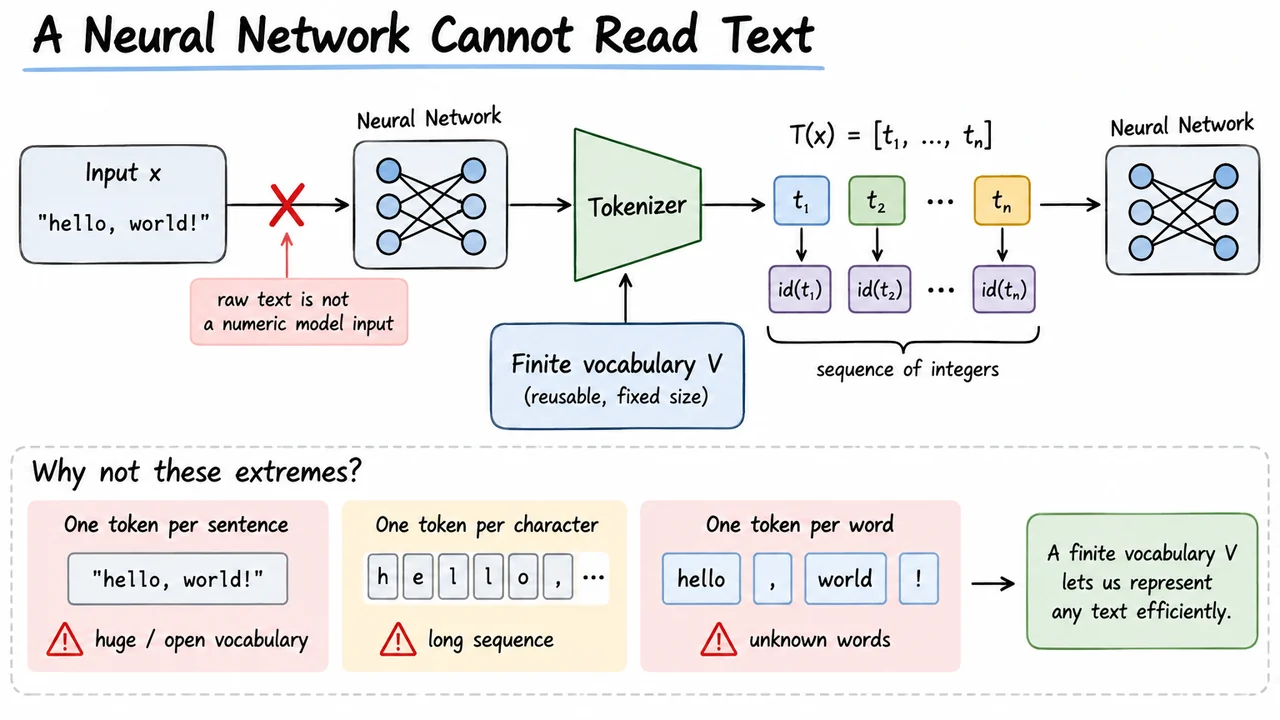
Type hello, world! into an LLM. To you, that string is already meaningful: two familiar words, a comma, a space, and an exclamation mark. To the neural network, however, it is not yet a usable model input. The network's layers operate on numbers—vectors and matrices—not on the abstract idea of a Unicode string. Before attention can compare anything or a feed-forward layer can transform anything, the text needs a deterministic numerical representation.
One extreme would be to assign a unique symbol to every possible sentence. Then hello, world! could become one integer and the sequence would be wonderfully short. But this immediately fails on new sentences: the set of possible strings is effectively unbounded, so no practical finite vocabulary could contain them all. At the opposite extreme, we could split everything into very small units such as characters. Coverage becomes easier, but ordinary text turns into long sequences, and Unicode makes the notion of a "character" less simple than it first appears. Whole-word tokenization has the reverse problem: common sentences become short, while names, inflections, typos, code identifiers, and newly coined words make the vocabulary open-ended.
Modern LLM tokenization therefore inserts a reusable symbolic layer between raw text and the neural network. Let the input string be . A tokenizer converts it into an ordered sequence
where every is chosen from a finite vocabulary , and is the number of tokens produced for this particular input. A token might happen to look like a whole word, a word fragment, punctuation, whitespace attached to a fragment, or something even less intuitive. The crucial property is not that tokens match human linguistic categories. It is that a limited collection of them can be recombined to represent a huge variety of text.
The next step is numerical. Each vocabulary entry has an integer index, which we write as . So a tokenizer does two conceptually separate things: it decides how to segment the text into reusable pieces, and it maps those pieces to stable integer IDs. Those integers are still not semantic quantities—you cannot infer that token 500 is somehow "more" than token 200—but they give the model a finite address space it can use.
This already exposes the central engineering tradeoff. Larger reusable pieces can make smaller, which is attractive because LLM context and computation are measured in token positions. Smaller pieces give stronger coverage of unfamiliar text but can lengthen the sequence. Tokenizer design is largely about finding a useful balance between those pressures while preserving the input faithfully.
We now have a string, a token sequence, and integer IDs. The remaining question is what each of those objects actually is—and how an integer ID becomes the vector that the transformer processes.
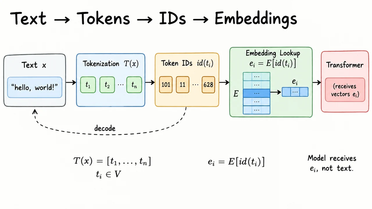
Take one token from the previous pipeline, say . The token itself is a symbolic vocabulary entry: perhaps hello, perhaps a fragment such as ing, perhaps punctuation, or perhaps a piece that includes whitespace. Its integer is only the address assigned to that entry inside the vocabulary. Those two objects are easy to conflate because tokenizer libraries often return IDs directly, but the distinction matters whenever we discuss what the model has actually learned.
For the complete input , the tokenizer gives
Imagine, purely illustratively, that hello, world! becomes four token strings and those strings have IDs [120, 847, 31, 9]. The particular numbers do not tell us that one token is closer in meaning to another, and a different tokenizer could assign completely different numbers to the same-looking strings. The IDs are categorical indices. Their purpose is to let the model address a finite table efficiently.
That table is the embedding matrix . For every token position, the model uses the integer ID to retrieve one row:
The result is a learned vector. Unlike the ID, its numerical coordinates can participate in neural-network operations. During model training, gradient descent adjusts these embedding vectors along with the rest of the model parameters, so the row associated with a token becomes useful in the contexts where that token occurs. The transformer therefore does not receive the literal string hello or the integer 120 as a meaningful scalar. It receives the vector stored at row 120 of , together with vectors for the other token positions.
This also explains why replacing a pretrained model's tokenizer is not a harmless preprocessing change. The model has learned an embedding row for each ID according to the vocabulary it was trained with. If a new tokenizer decides that ID 120 means something else, the model still retrieves the old row 120. The numerical interface and the vocabulary must agree. Later we will return to this coupling when discussing tokenizer evaluation.
Decoding travels along a different path. If the model produces a sequence of token IDs, the tokenizer can map those IDs back to token strings and then reconstruct text according to its encoding rules. It does not invert the embedding vectors to recover words. An embedding is a learned internal representation, not a reversible encoding of the token's spelling.
So there are four distinct layers in the pipeline: raw text, token strings, token IDs, and embedding vectors. Once those are kept separate, the next design problem becomes sharper. The model needs a finite vocabulary , but what should its entries be? Very small character-like pieces, entire words, or something between the two?
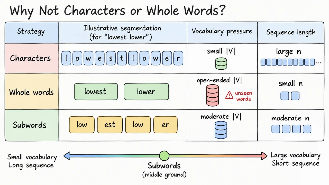
Consider the tiny phrase lowest lower. If we make every character a token, an illustrative segmentation is l | o | w | e | s | t | space | l | o | w | e | r. The vocabulary can remain relatively small because the same letters are reused everywhere, but the sequence is long. Every extra position matters to a transformer: it occupies context and gives the model another position to process. Character-level tokenization therefore buys broad compositional coverage by spending more sequence length.
Now push in the opposite direction and make every whole word a token. The same phrase becomes simply lowest | lower, which is compact. The problem moves into the vocabulary. Natural language does not have a neat, closed list of possible word forms: lower, lowering, lowered, names, URLs, typos, domain jargon, code identifiers, and arbitrary strings keep extending it. A whole-word tokenizer must either grow an enormous vocabulary or introduce some mechanism for words it has never seen.
Subword tokenization occupies the useful middle. An illustrative segmentation might be low | est | low | er. The piece low can be reused in both words, while est and er capture common continuations. This reduces the number of positions compared with characters without demanding a separate vocabulary entry for every full word. A rare new word can still be assembled from smaller pieces when no convenient larger token exists.
This compromise creates an important tension between vocabulary size and sequence length . If contains more large, frequently occurring chunks, many inputs can be expressed using fewer tokens. But those extra vocabulary entries enlarge the model's embedding and output interfaces, and a finite vocabulary can never memorize every useful string. If contains mostly tiny pieces, the vocabulary is easier to cover broadly but ordinary text takes more token positions. There is no single segmentation scale that wins everywhere.
It is also worth resisting a linguistic interpretation that sounds plausible at first. A subword tokenizer is not necessarily trying to discover prefixes, suffixes, roots, or other "true" pieces of language. Sometimes a learned token aligns beautifully with a morpheme such as ing; sometimes it captures a frequent letter sequence whose boundary would look arbitrary to a linguist. The training procedure is usually optimizing statistical reuse under a vocabulary budget, not reconstructing a grammar textbook.
That distinction becomes concrete if we place the same sentence under character, word, and subword segmentations side by side. The text has not changed; only the interface between the text and the model has.
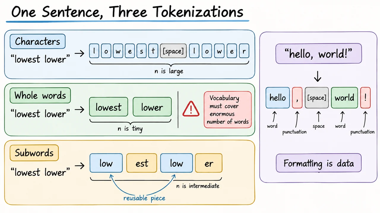
Write the three segmentations explicitly and the tradeoff becomes visible. Under a character-like scheme, the phrase can be represented as
That is twelve token positions in this simplified example. The advantage is reuse: the letters needed for lowest are mostly the same letters needed for lower, and an unfamiliar related word can still be spelled out. The disadvantage is that the transformer must process many positions to represent a very short phrase.
At the whole-word extreme, the same text becomes
Now the sequence has only two positions. But the apparent efficiency depends on both complete words already belonging to . Change the input to lowest lowers, a person's surname, or an unseen technical term and a pure whole-word vocabulary needs some escape hatch. The short sequence has been purchased by placing much more responsibility on the vocabulary.
A subword scheme can instead produce something like
Four positions are longer than the whole-word representation but far shorter than the character representation. More importantly, low is reused. If the tokenizer later sees another word containing a compatible occurrence of that piece, the same vocabulary entry may help encode it. These particular boundaries are illustrative; a real tokenizer could split the phrase differently because its segmentation depends on its learned vocabulary and rules.
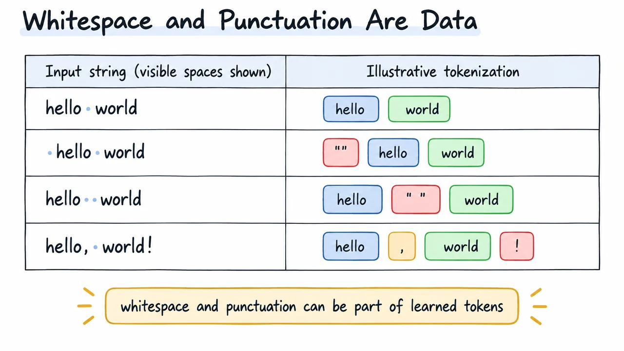
Now return to hello, world!. Even before choosing a particular algorithm, this example exposes something that word-only intuition tends to hide. The comma, the exclamation mark, and the space between the words all belong to the input string. A lossless tokenizer has to account for them somehow. Depending on the tokenizer, punctuation may be separate tokens, whitespace may be bundled into neighboring tokens, or several characters may be grouped together. The fact that a human visually treats the space as "nothing" does not remove it from the data.
So segmentation is doing more than finding word boundaries. It defines the discrete alphabet through which every kind of text—words, formatting, punctuation, code, and eventually arbitrary Unicode—reaches the model. The remaining question is where those useful pieces such as low, est, or er come from. Rather than hand-designing them, modern tokenizers usually learn their vocabulary from a corpus.
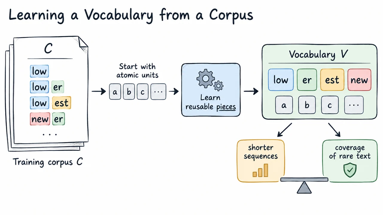
Suppose our tokenizer training corpus contains low, lower, lowest, and newer, with some words appearing more often than others. If we start from tiny atomic units, the trainer can notice that certain adjacent sequences recur. The letters forming low, for example, appear across several related strings. Turning a recurring sequence into one vocabulary entry can shorten many encoded examples at once, which makes that entry more valuable than memorizing an equally long sequence that appears only once.
This is the basic idea behind training a tokenizer. The tokenizer is usually learned before the language model itself is trained. Its trainer scans a corpus, constructs a finite vocabulary , and records whatever rules are needed to segment future text using that vocabulary. The exact optimization differs across BPE, WordPiece, and Unigram, but all of them must answer a similar allocation problem: with only available entries, which strings deserve to become reusable tokens?
Frequency helps, but simply storing the longest or most frequent full strings would be a poor solution. Imagine spending most of on complete sentences from . Those sentences would encode very compactly, but a slightly different sentence would lose that benefit and might become impossible to express if no smaller fallback units remained. A robust tokenizer therefore needs a hierarchy of reusable pieces: common larger chunks for compression and sufficiently small units for coverage of rare or novel text.
The composition of matters directly. If the corpus contains huge amounts of English prose, common English fragments get many opportunities to justify vocabulary entries. If code, Hindi, Japanese, legal terminology, mathematical notation, or biomedical names are scarce, the learned vocabulary may allocate fewer convenient pieces to those domains. The tokenizer can still represent them if its base units provide coverage, but it may need more tokens to do so. This is one reason tokenizer efficiency is never completely separable from the data used to train it.
There is also a useful distinction between tokenizer training and language-model training. The tokenizer trainer decides the discrete alphabet and segmentation rules. Once those are fixed, the LLM sees sequences of token IDs generated by that interface and learns its embeddings and higher-level parameters around them. Changing the tokenizer later changes the meaning of those discrete inputs, which is why the choice becomes part of the model's architecture in practice.
We can now make the vocabulary-learning process concrete. One of the simplest and most influential strategies is Byte Pair Encoding, or BPE: start small, count which neighboring pieces occur together most often, merge the most frequent pair, and repeat.
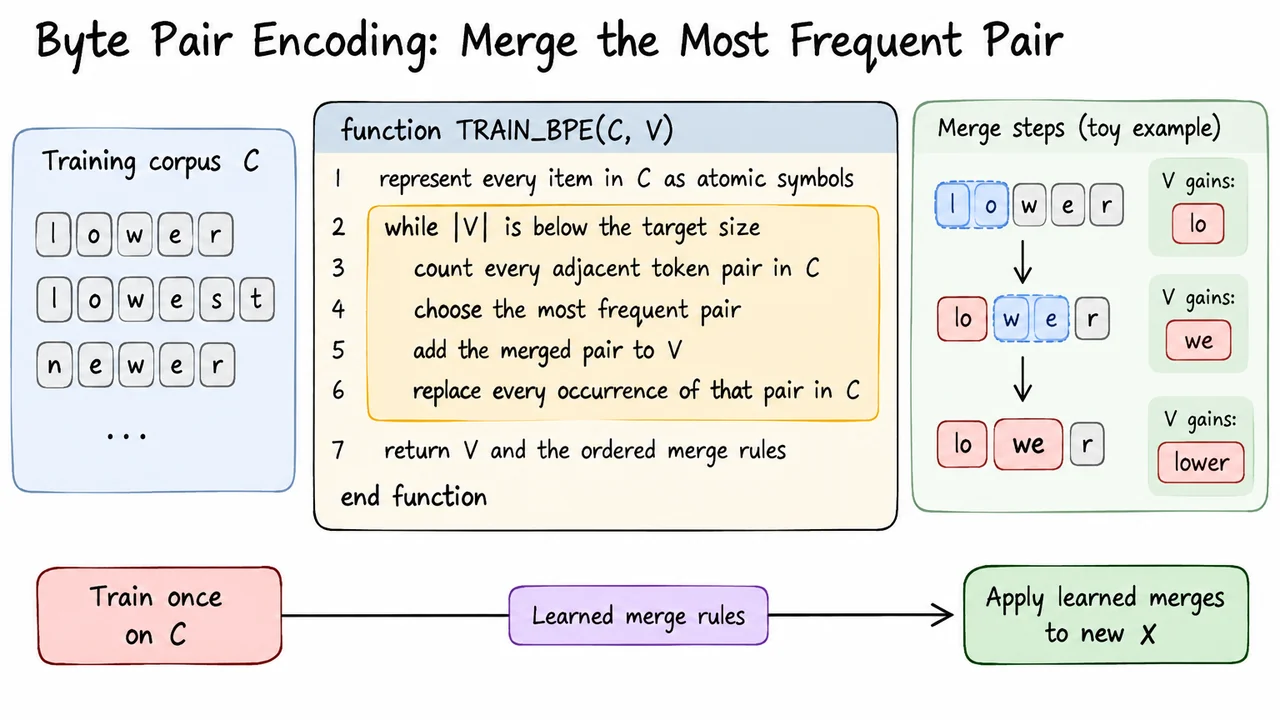
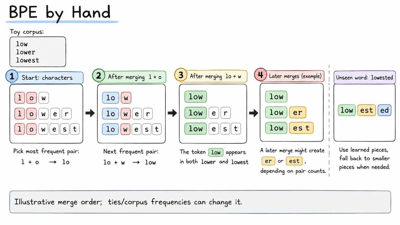
BPE turns the idea of "promote useful recurring pieces" into a greedy procedure. Begin by representing the training corpus using small atomic symbols. For a toy character-based version, low starts as l | o | w, lower as l | o | w | e | r, and so on. At this point the vocabulary contains the atomic units, but none of the larger chunks such as lo or low yet exist as single tokens.
The trainer now counts adjacent pairs in the current representation of the corpus. If l | o occurs more often than any other neighboring pair, BPE creates a new vocabulary entry lo. It then rewrites every eligible occurrence of l | o as that single new symbol. After this rewrite, the corpus representation itself has changed, so the next round of pair counts is performed on the new symbols. A pair such as lo | w can now exist even though lo did not exist at the beginning.
The loop is conceptually simple:
The greedy part matters. BPE does not search over every possible final vocabulary and choose the globally optimal one. Each step commits to a merge using the statistics available at that moment. Once l and o become lo, later pair counts operate on lo as an indivisible symbol. The ordering of merges therefore becomes part of the learned tokenizer, and tie-breaking or differences in the training corpus can eventually produce different vocabularies.
It is equally important to separate training from encoding. During tokenizer training, BPE repeatedly counts pairs in to discover and order merge rules. When we later tokenize a new input , we do not train BPE again or count which pairs happen to be frequent inside that one prompt. The encoder starts from the tokenizer's base representation and applies the already learned merge rules according to the tokenizer's procedure. That is what makes tokenization deterministic for a fixed tokenizer configuration.
The result is a vocabulary containing a mixture of small foundational units and larger pieces that earned their place through repeated occurrence. Common patterns can collapse into single tokens, while uncommon strings remain decomposable into smaller pieces. The easiest way to make this mechanism intuitive is to run a few merge steps by hand and watch low emerge from l, o, and w.
Use a deliberately small corpus so we can see every decision. Suppose low, lower, and lowest occur often enough that the adjacent pair l | o wins the first BPE count. The trainer creates the token lo, and those words are rewritten as lo | w, lo | w | e | r, and lo | w | e | s | t. Nothing semantic has been declared about lo; it has simply become a convenient unit because the corpus repeatedly contained those two neighbors.
Now count pairs again. If lo | w is the most frequent pair in the rewritten corpus, BPE merges it into low. The same new token immediately helps several words:
low can now be one token.lower begins as low | e | r.lowest begins as low | e | s | t.One vocabulary entry has shortened multiple strings because the strings share a repeated prefix. This is the core economy BPE is exploiting.
Later rounds might merge e | r into er, giving lower → low | er, or build est through some sequence of merges, giving lowest → low | est. Which one happens first depends on actual pair frequencies in , and ties need some deterministic rule. With a different corpus, perhaps newer appears frequently enough that merges involving new or er become more attractive. There is no corpus-independent list of the "correct" BPE pieces.
Now imagine encoding a related string that was not present during tokenizer training. Suppose the vocabulary contains low and er but not the entire new word. The encoder can still use the learned larger pieces where they apply and fall back to smaller vocabulary entries elsewhere. That is why a subword vocabulary generalizes beyond the strings it memorized: it retains compositional building blocks underneath the larger chunks.
This example also shows why inspecting only the final vocabulary hides part of BPE's behavior. The merge order matters because larger tokens are constructed from earlier units. Two BPE tokenizers can begin from similar base symbols yet learn different merge sequences and therefore segment the same text differently. Corpus frequencies, preprocessing, vocabulary budget, and tie-breaking can all change the path.
So BPE solves one problem elegantly: it grows reusable chunks from repeated local patterns. It does not, by itself, settle what the smallest starting units should be. If those units are ordinary characters and an unseen Unicode symbol falls outside the base vocabulary, coverage can still become awkward. Byte-level BPE moves the foundation one layer lower.
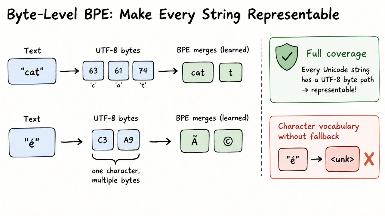
Moving the base representation to bytes gives us a clean coverage guarantee. Unicode text is encoded as UTF-8, and UTF-8 expresses every valid Unicode string as a sequence of byte values. Instead of requiring the tokenizer's initial vocabulary to contain every character or script it might ever encounter, a byte-level tokenizer can begin from a finite byte-based alphabet and learn larger BPE merges on top of it.
For ordinary ASCII text, this often feels unsurprising because each ASCII character occupies one UTF-8 byte. A word such as cat starts from byte values corresponding to c, a, and t, after which learned merges may combine them into larger units. For non-ASCII text, the distinction becomes more visible. A single accented character, a Devanagari character, or an emoji can require multiple UTF-8 bytes. Before larger merges apply, one human-visible symbol may therefore correspond to several base units.
The practical benefit appears when the tokenizer encounters something rare. Suppose a character never appeared often enough during tokenizer training to earn a convenient larger token. A byte-level scheme does not need to replace it with an information-destroying "unknown character" merely because the character itself is absent from . The character still has a UTF-8 byte representation, so the encoder can fall back to smaller byte-derived pieces. Decoding those pieces reconstructs the original byte sequence and therefore the original text, assuming the tokenizer's normal reversible encoding rules.
This does not mean every Unicode character becomes one token. In fact, the opposite is often true for rare text. Frequently observed byte sequences may be merged into compact tokens, while unfamiliar sequences can expand into several tokens. The guarantee is about representability, not efficiency. A language or symbol can be perfectly representable and still consume many more token positions than common training-corpus text.
Byte-level tokenization also explains some strange-looking tokenizer displays. A token boundary may cut through the UTF-8 representation of what you perceive as one character, so an inspection tool may show fragments that do not look like valid standalone text. That is not necessarily corruption. The token is fundamentally an element of the model's discrete vocabulary; its human-readable rendering is secondary.
We have now changed one dimension of BPE—the foundation from which merges are built—without changing its basic greedy merge idea. Other tokenizer families alter a different dimension: how they decide which larger subwords deserve vocabulary entries in the first place.
WordPiece can look deceptively similar to BPE when you inspect only the final segmentation. A word might be broken into a familiar-looking stem and one or two continuations, and both systems may end with vocabularies full of reusable subwords. The difference lies in how those pieces earn their place during vocabulary construction.
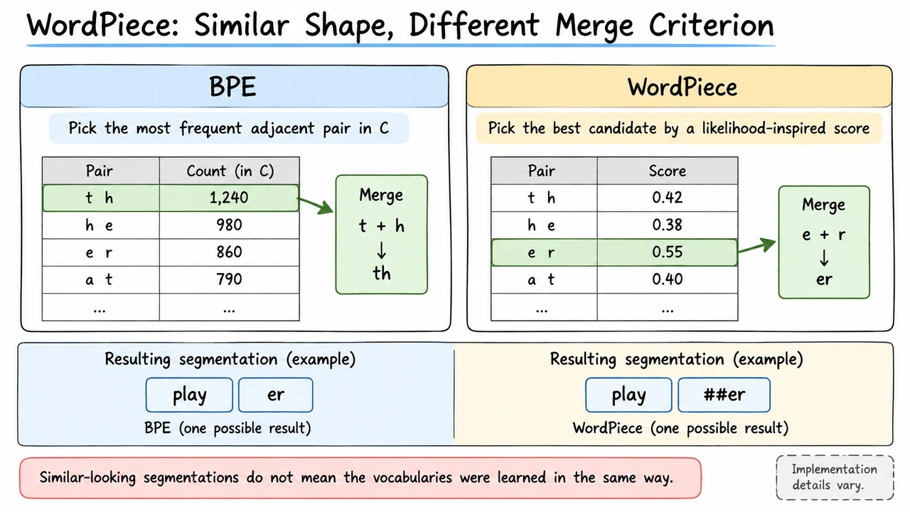
BPE's core greedy signal is straightforward: count adjacent pairs and merge the pair with the highest frequency. A pair that appears often is attractive because collapsing it saves token positions in many places. WordPiece uses a likelihood-inspired criterion instead. Conceptually, it asks whether adding a candidate combined piece improves the model of the training text enough to justify that vocabulary entry. Raw pair frequency contributes information, but it is not by itself the complete selection rule.
This matters because a pair can be common simply because its individual components are already extremely common. Another pair may occur fewer times yet represent a more distinctive association between its parts. A likelihood-inspired score can therefore rank candidates differently from pure frequency. Two trainers operating on the same corpus can end up choosing different subwords even though both are trying to build a compact reusable vocabulary .
You may also encounter surface conventions associated with WordPiece. Some implementations mark tokens that continue a word with a prefix such as ##. An illustrative segmentation might render a word as low | ##er, where the marker indicates that er occurs inside a word rather than beginning a new one. That marker is part of the tokenizer's representation convention; it should not be confused with the essential definition of WordPiece, and exact conventions differ across tokenizers.
The broader lesson is that final token strings do not tell you the entire algorithmic story. Seeing play | ##ing in one tokenizer and play | ing in another does not mean the two vocabularies were learned in the same way. Preprocessing rules, candidate scoring, training corpus, vocabulary size, and boundary conventions all shape the result.
BPE builds upward through a sequence of greedy merges. WordPiece also constructs reusable subwords but evaluates candidate combinations differently. A third major family, Unigram, changes the direction of the search more radically: rather than starting tiny and repeatedly adding pieces, it begins with many candidate pieces and removes the ones it can afford to lose.
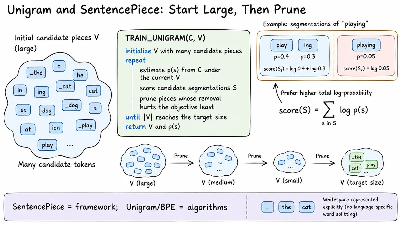
Unigram approaches vocabulary construction from the opposite direction. Instead of beginning with tiny units and growing one merge at a time, it starts with a relatively large collection of candidate token strings. Several different segmentations of the same text may therefore be possible at once. The training problem becomes: which candidate pieces make the corpus probable enough to keep, and which can be removed with little damage?
Assign each candidate token string a probability . If is one possible segmentation of an input, the tokenizer can score that segmentation by adding the log-probabilities of its pieces:
Because log-probabilities add, a segmentation made from well-supported pieces receives a larger score than one relying on collectively unlikely pieces. In practice, the model can evaluate alternative ways of partitioning the same string and prefer a high-scoring path rather than committing to one irreversible merge history as BPE does.
Training then becomes iterative. Start with many candidates in , estimate their probabilities from the corpus , evaluate how the corpus can be segmented under that vocabulary, and ask what would happen if particular candidates disappeared. Pieces whose removal hurts the objective least are pruned. The trainer re-estimates probabilities and repeats the process until reaches the desired size. The important intuition is that a token survives because the vocabulary as a whole works noticeably worse without it.
This also gives Unigram a different relationship to ambiguity. Suppose a string can be segmented as low | est or lo | west under the current candidate set. BPE's learned merge order tends to determine a particular segmentation procedure. A Unigram model instead has explicit probabilities over pieces and can compare competing segmentations through their scores. Implementations can use this probabilistic structure in different ways during training or encoding, but the central idea is whole-segmentation competition rather than a single greedy merge sequence.
One terminology trap is worth fixing now: SentencePiece is not the name of this algorithm. SentencePiece is a tokenizer framework that can train a Unigram model, but it can also implement BPE. One useful design choice associated with SentencePiece is that it can operate directly on raw text and represent spaces explicitly, instead of requiring a language-specific word splitter before subword learning. That becomes important as soon as we leave clean toy words and return to real prompts.
We now have three ways of learning subwords—BPE, WordPiece, and Unigram—and none of them gives whitespace or punctuation a free pass. Those characters are part of the input, and small formatting changes can alter the token sequence.
Compare four inputs that differ only slightly: hello world, hello world, hello world, and hello, world!. To a human, the first three express essentially the same two words. To a tokenizer, they are different byte or character sequences, so there is no reason their token boundaries must match.
Many modern tokenizers make whitespace boundaries statistically useful. A vocabulary entry might effectively represent a word together with the space that tends to precede it, rather than storing the bare word alone. Under such a scheme, world at the beginning of a string can tokenize differently from world after another word. The exact representation varies by tokenizer, but the general consequence is stable: adding one leading space can change an existing token rather than merely insert one extra "space token."
Repeated spaces make the point even clearer. In hello world, the second space is part of the input and must survive a reversible encoding somehow. Depending on the learned vocabulary and preprocessing rules, those two spaces might be grouped, split, or attached differently to neighboring pieces. Therefore the new token count is not reliably equal to the old token count plus one. A tiny textual edit can rearrange several token boundaries.
Punctuation behaves similarly. The comma in hello, world! and the exclamation mark at the end may each form their own tokens, join neighboring fragments, or participate in larger learned chunks. What matters is corpus statistics and tokenizer rules, not our visual sense that punctuation is secondary to the words. The same logic applies to newlines, tabs, Markdown markers, JSON syntax, and indentation in source code.
This has practical consequences whenever someone estimates tokens from visible word count. A thousand-word document with ordinary prose may tokenize very differently from a thousand-word document containing tables, unusual spacing, URLs, or code. Copy-pasting text from another application can introduce formatting that changes even when the text looks nearly unchanged. Chat systems add another source of invisible structure because the interface may serialize messages with separators and control text that users never see directly.
The safe mental model is simple: the tokenizer receives an exact string representation, not your interpretation of what parts of the formatting "matter." If a character is present—or if the application's serialization inserts it—it can affect segmentation. Unicode takes this one step further, because even the idea of "one visible character" can hide several different computational units.
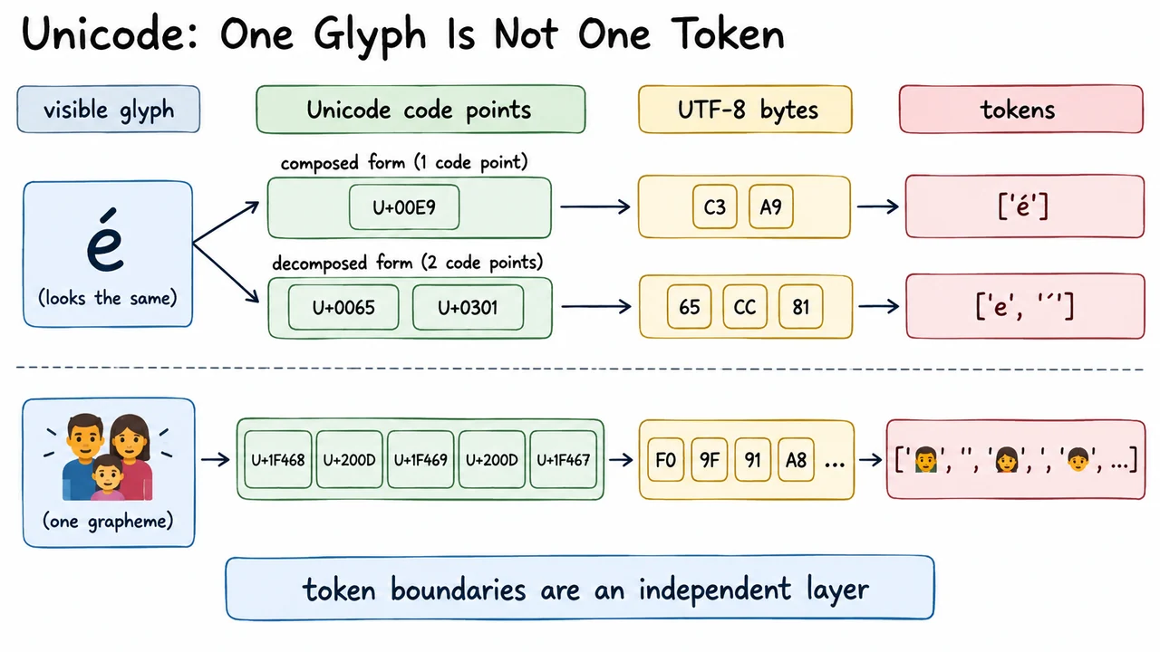
A screen renders graphemes—the user-perceived characters—but those are not the same thing as Unicode code points, and code points are not the same thing as UTF-8 bytes. Tokenization sits above all of these layers. That is why a statement such as "this emoji is one character, so it should be one token" has no reliable basis.
Take an accented letter as a simple example. Unicode may represent what appears to be the same visible glyph in a composed form using one code point, or in a decomposed form using a base letter followed by a combining accent. A human reader may not notice any difference. Computationally, however, the code-point sequences differ, and their UTF-8 byte sequences differ as well. Unless a tokenizer's normalization step deliberately maps those forms to the same representation, they can produce different tokenizations.
Normalization therefore matters, but it should not be treated as a universal hidden cleanup step. Different tokenizer pipelines make different choices about Unicode normalization and other preprocessing. Some distinctions may be collapsed; others may be preserved because the model was trained to see them. If you normalize text differently from the model's expected pipeline, you can change before subword segmentation even begins.
Emoji make the layering more obvious. A single displayed emoji can be assembled from several Unicode code points: a base symbol can combine with variation selectors, skin-tone modifiers, or zero-width joiner sequences that visually connect multiple components. Those code points then become multiple UTF-8 bytes. A byte-level tokenizer may merge frequently occurring portions of that byte sequence, leave rarer portions fragmented, or even place token boundaries inside what the user experiences as one grapheme.
So there are at least four useful levels to keep separate: the visible glyph, the Unicode code-point sequence, the UTF-8 byte sequence, and the model's token sequence . A boundary at one layer does not force a boundary at the next. One glyph can become many code points; one code point can become several bytes; several bytes can be merged into one token; and a single visible grapheme can span multiple tokens.
This is not merely a Unicode trivia problem. It affects token counts, equality checks, multilingual processing, adversarial text handling, and debugging. Two strings that look identical can occupy different token budgets if their underlying representations differ. Once we care about languages beyond the tokenizer's dominant training distribution, these differences also expose a broader efficiency question: how many tokens does the tokenizer need to express the same amount of linguistic content?
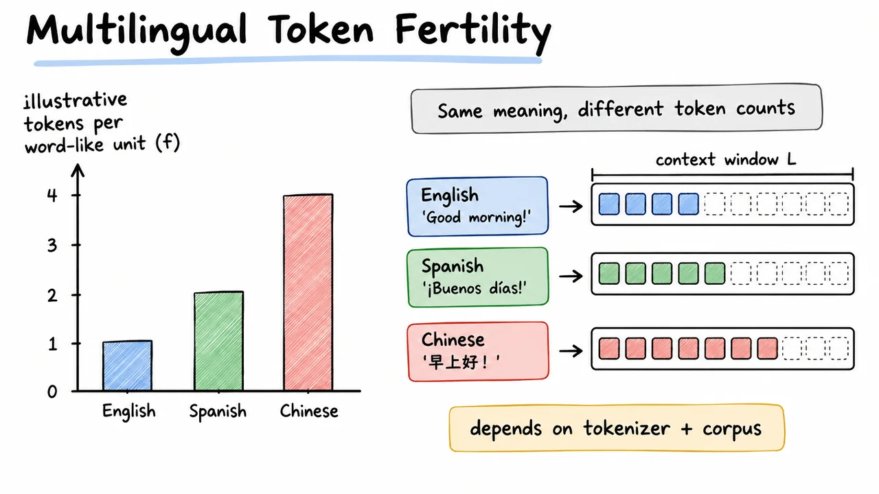
Suppose two people express roughly the same message in two different languages. The semantic content may be comparable, yet one version could occupy substantially more token positions than the other. Nothing is "wrong" with the longer language. The difference can come from how the tokenizer's finite vocabulary was allocated during training.
To measure this, we can use token fertility. For a representative corpus sample, let be the total number of produced tokens. Choose a consistent notion of word-like units for that corpus, then define as the number of tokens per such unit. A lower means the tokenizer typically needs fewer tokens to represent each chosen word-like unit; a higher means the text is more fragmented. The definition is intentionally corpus-dependent because "word" boundaries themselves are not equally natural across all writing systems.
Why does fertility differ? Imagine that the tokenizer's training corpus contains abundant English. Frequent English words, stems, punctuation patterns, and common byte sequences have many chances to earn compact entries in . If another language receives much less representation, its text may still be perfectly encodable—especially with byte fallback—but the tokenizer may assemble it from smaller pieces. The same phenomenon can occur within one language across domains: ordinary prose may tokenize compactly while specialist chemical names or source code fragment heavily.
The consequence is more than aesthetic. A model with context limit counts token positions, not sentences or semantic units. If one corpus has higher fertility, less source material fits into the same . The model may need more positions to read an equivalent amount of content, which can increase memory use, latency, and token-priced API cost. A nominal 100,000-token context window therefore does not translate into one universal number of pages or words across languages.
Fertility should not be turned into a simplistic ranking of languages. It depends on the exact tokenizer, its corpus , normalization rules, vocabulary size, and the evaluation sample. A newer tokenizer trained with broader multilingual coverage can reverse patterns seen in an older one. Even within the same language, conversational text, legal text, and code-switching can have different fertility.
The practical rule is to measure rather than assume. If your application serves multiple languages, build representative samples for each and compare how many tokens the actual production tokenizer emits. That same discipline becomes especially useful in two domains where human units are deceptively obvious but tokenizer units often are not: numbers and programming code.
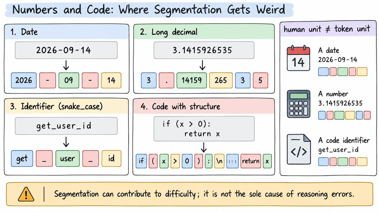
Look at the date 2026-09-14. A person sees three semantic fields—year, month, day—separated by hyphens. A tokenizer has no obligation to preserve those fields. Depending on its learned vocabulary, it might group several digits together, split some digits individually, and treat the hyphens as separate pieces. Another tokenizer can choose different boundaries for the exact same date. The grouping is driven by training statistics and preprocessing rules, not by an understanding of calendars.
Long numbers expose the same mismatch. A decimal such as 3.1415926535 may be segmented into a mixture of multi-digit chunks, punctuation, and single digits. Those boundaries need not line up with place value or any arithmetic decomposition that would be convenient for calculation. This does not prove that tokenization is the cause of an LLM's arithmetic mistakes, but it does mean the model may receive numerical strings in units that are awkward from a mathematical perspective.
Programming identifiers create a similar problem. get_user_id has meaningful structure for a programmer: words separated by underscores. A tokenizer trained on enough code may learn useful pieces around those patterns, but it could also split the identifier in less intuitive places. A camelCase version such as getUserId presents different character statistics, so its boundaries can differ again. Long hashes, UUIDs, generated variable names, and minified code are especially likely to lack convenient reusable chunks.
The surrounding syntax also counts. Consider a small indented function. Spaces used for indentation, newlines, parentheses, commas, operators, braces, quotes, and comments all enter the tokenizer's input. Even when the logical program is short, formatting can produce many token positions. A tokenizer whose corpus contains substantial code can devote vocabulary capacity to common operators and code fragments, reducing this overhead; a tokenizer tuned mostly to prose may not.
This helps explain why evaluating "tokens per word" alone is insufficient for developer tools. Code has no single natural word unit, and numerical tasks can be dominated by strings that look compact to a human but fragment heavily. For these domains, inspect actual sequence lengths , common identifier patterns, numeric formats, whitespace behavior, and worst-case examples.
Keep the causal claim modest. Better numerical or code-aligned tokenization can shorten sequences and present the model with more convenient recurring units, but it does not automatically give the transformer arithmetic algorithms or programming competence. Tokenization shapes the interface; reasoning quality also depends on the model, training data, objectives, and inference process. The next interface detail is even more structural: some vocabulary entries do not represent ordinary text at all.
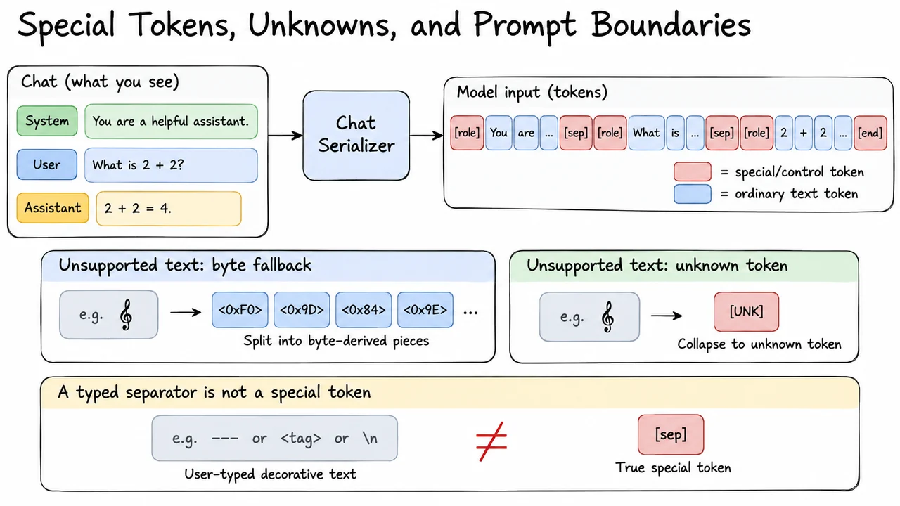
A vocabulary can contain entries that are not meant to represent ordinary user text at all. Models often reserve special tokens for structural purposes: beginning or end markers, message roles, separators, padding, masks, tool boundaries, or other protocol-specific signals. These tokens still have IDs and embeddings, but their job is to tell the model something about the structure of the sequence rather than spell part of a sentence.
This becomes especially important in chat models. The conversation you see as separate system, user, assistant, and tool messages is typically serialized into one model input using a model-specific template. That serialization can insert role markers, separators, end-of-message markers, or other text/token structure around the visible content. Those hidden additions consume token positions under the same context limit . So counting only the words visible in the chat box can underestimate the sequence the model actually receives.
There is a security-relevant distinction here. If an application types a decorative string such as ---SYSTEM---, an XML-like tag, or several newlines inside ordinary user content, those characters are still ordinary input unless the model's protocol explicitly gives them special treatment. They do not automatically become the same thing as a reserved system-role token. Applications should therefore use the model's official chat or template encoding rather than trying to recreate privileged boundaries by inventing textual delimiters.
Unsupported text presents another tokenizer-design choice. A tokenizer with a sufficiently complete byte fallback can preserve unusual Unicode through smaller byte-derived pieces. Other tokenizer schemes may have an unknown token representing content that cannot be expressed with the ordinary vocabulary. When several distinct unsupported strings all collapse to the same unknown ID, information is lost before the model sees it. Modern byte-based approaches are attractive partly because they can avoid that failure mode for arbitrary UTF-8 text.
Special tokens must also be handled carefully during encoding and decoding. Some libraries prevent ordinary user text from being interpreted as reserved tokens unless explicitly allowed, precisely because a literal string that resembles a control marker should not necessarily acquire control semantics. The correct behavior is model- and tokenizer-specific; manually concatenating IDs or guessing special strings can silently produce inputs the model was never trained to interpret that way.
At this point the tokenizer is no longer just a compression utility. It defines part of the protocol between the application and the model: which text pieces exist, which structural markers exist, and how a conversation becomes one token sequence. Once that full sequence is assembled, its length becomes a concrete systems quantity—one that determines how much fits in context and how much computation the model performs.
After the application has serialized the conversation, the model receives one ordered sequence of token positions:
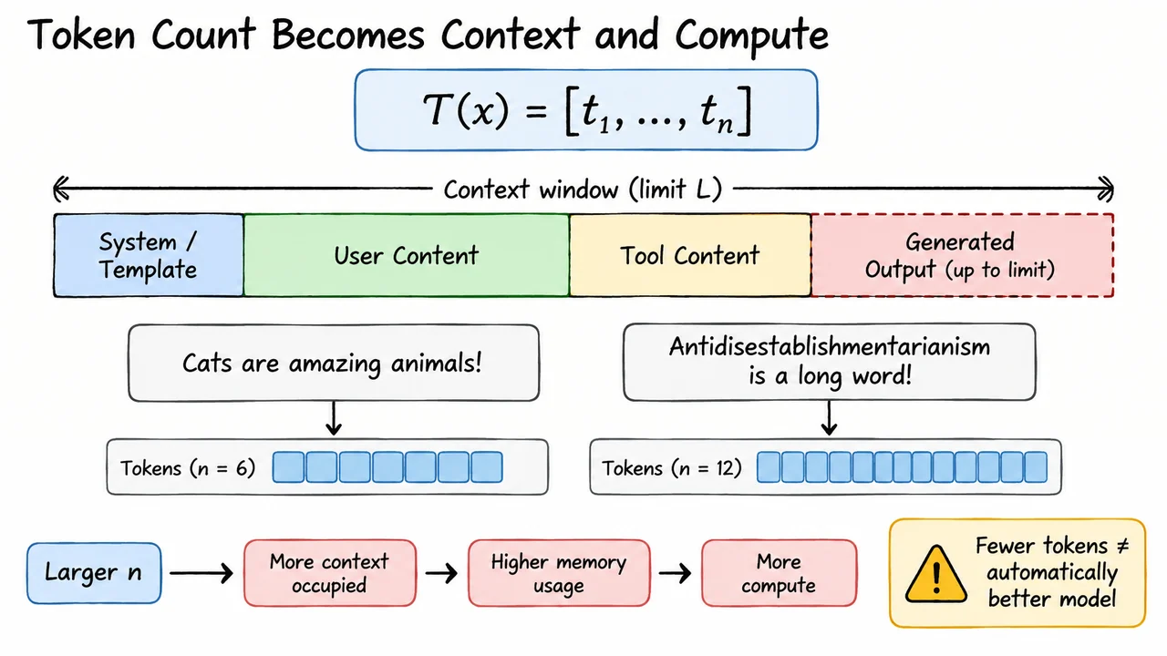
The number is now operational, not merely descriptive. The model's maximum context length is measured in tokens, so system instructions, message-role markers, user text, retrieved documents, tool outputs, and the generated continuation all compete for the same finite budget. A prompt that looks short in characters can still consume a surprising fraction of if its language, formatting, code, or Unicode content fragments heavily.
This is why character count and word count are unreliable proxies for context usage. Two files can contain the same number of characters while producing very different values of . A compact-looking source-code file may contain punctuation and identifiers that split aggressively; a longer passage of common prose may contain highly reusable vocabulary pieces. The tokenizer—not visual length—determines how many positions reach the transformer.
Sequence length also affects computation. Every token position needs an embedding and participates in the transformer's layers. Attention mechanisms create interactions among positions, while other operations also scale with the number of positions being processed. Exact performance depends on model architecture, implementation, caching, hardware, and whether we are processing a prompt or generating incrementally, so there is no single universal cost formula here. The robust statement is that longer token sequences demand more model work and memory than shorter representations of otherwise comparable input.
That creates a practical benefit for token-efficient vocabularies. If your domain is represented using fewer tokens, more source material can fit under the same , and the model may process that material with less sequence overhead. For multilingual systems, code assistants, or document-heavy applications, those savings can accumulate across every request.
But compression cannot be optimized in isolation. A trivial tokenizer that turned every frequently seen paragraph into one giant token could make some sequences extremely short while exploding vocabulary requirements and generalizing poorly to variations. Larger also changes the model's embedding and output interfaces. Good tokenizer design therefore balances compact sequences with reusable, compositional pieces and adequate coverage.
Once token count is treated as the real resource, we can quantify tokenizer efficiency more systematically. Two simple measurements—bytes per token and token fertility—let us compare representations on a corpus, and token-priced APIs make the economic consequence direct.
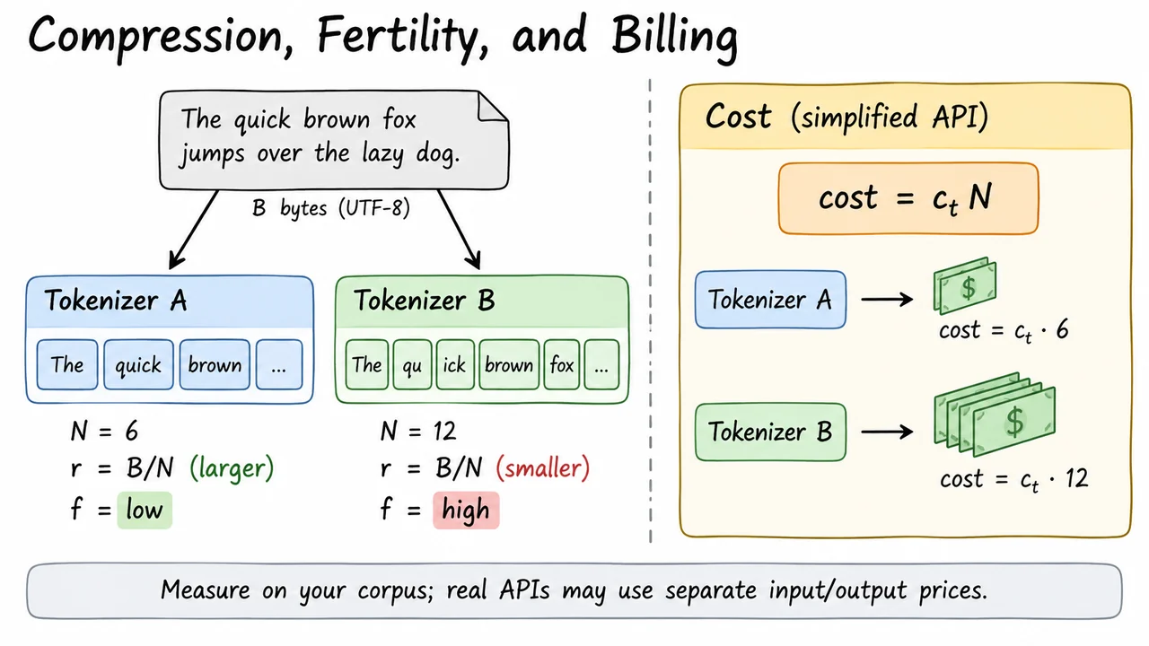
Take one representative corpus sample and hold the source text fixed. Let be its length in UTF-8 bytes, and let be the number of tokens a particular tokenizer produces. A simple way to summarize compression is
This tells us how many source bytes, on average, are packed into each token for that sample. If tokenizer A produces 250 tokens for the same where tokenizer B produces 400, then A has a larger . It is using fewer model positions to carry the same byte sequence. The metric is intentionally mechanical: it does not claim that those tokens are linguistically better or that the model will reason better from them.
Token fertility measures a related quantity from the perspective of word-like units rather than bytes. Suppose we choose a consistent way to count word-like units in the evaluation corpus. Then lower fertility means the tokenizer emits fewer tokens per unit; higher fertility means the text is more fragmented. This is especially useful when comparing languages or domains, but only if the denominator is defined consistently enough to make the comparison meaningful. For scripts where "word" segmentation is ambiguous, bytes per token can sometimes be the cleaner cross-corpus measurement.
The two metrics answer slightly different questions. A tokenizer can have good byte compression while still splitting certain domain-specific entities awkwardly, and fertility can hide expensive punctuation, markup, or binary-looking strings that do not fit a normal word count. For a production system, it is therefore better to report several views together: total , , fertility where appropriate, and the tail of unusually expensive examples. Averages alone can conceal the exact prompts that overflow a context window.
Token pricing makes the consequence easy to see. In the simplest hypothetical API, suppose every token costs the same amount . Then usage cost is
If two tokenizers encode identical source text into different values of , their context consumption and this simplified bill differ proportionally. A tokenizer that reduces by 20% would reduce the token-count component of this toy cost by 20% for that fixed text. Real APIs are often more complicated: input and output tokens may have different prices, cached tokens may be priced differently, and some systems have additional accounting rules. The equation is a baseline model, not a universal billing formula.
This gives us a useful evaluation discipline. Do not ask whether one tokenizer is "more compressed" in the abstract. Take the actual languages, code, documents, chat templates, and retrieval payloads your application will send; tokenize them with the exact candidate tokenizers; and compare , , fertility, and the worst cases. The same tokenizer can look excellent on English prose and much less efficient on another language, codebase, or numerical workload.
These measurements also explain why token counts quoted by two model vendors are not directly comparable without knowing the tokenizer. The source string may be identical while differs because the underlying text interface differs. To understand that variation, we need to look at every choice that determines , not just whether the tokenizer is described broadly as BPE-like.
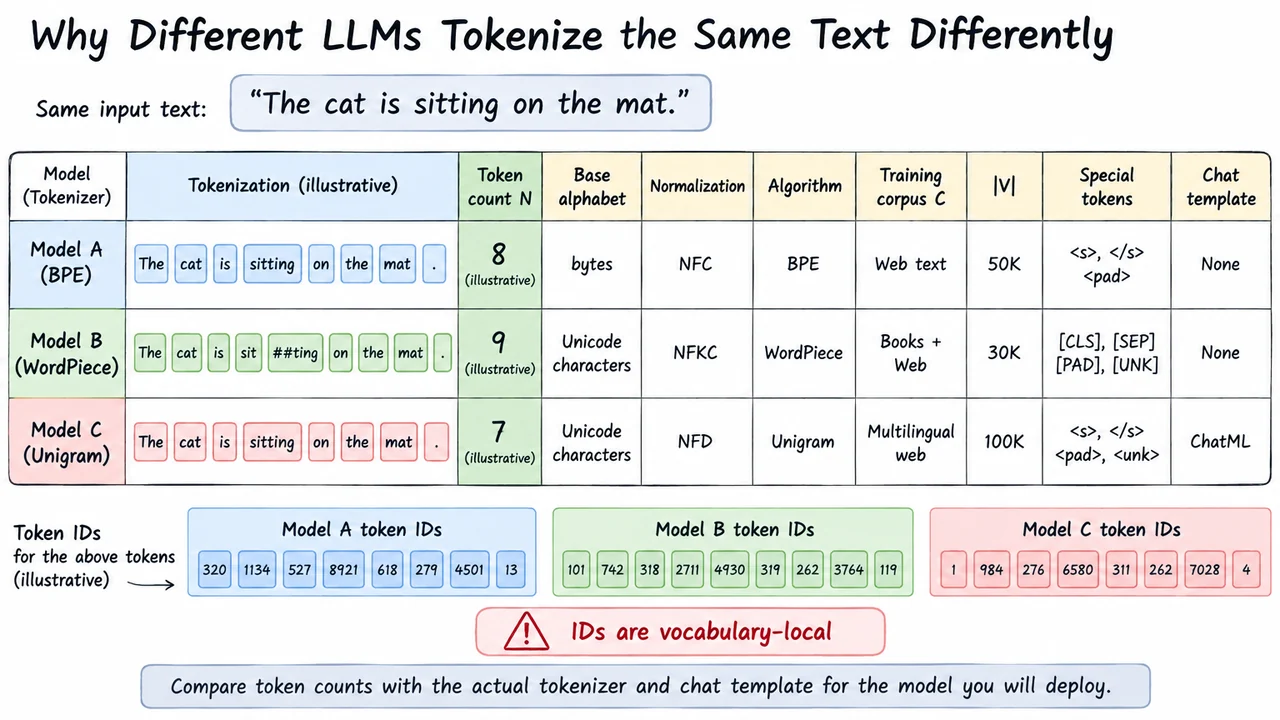
Take the exact same string—say hello, world!—and run it through three different production tokenizers. It is entirely normal for them to return different token counts, different boundaries, and completely different integer IDs. There is no universal decomposition waiting to be discovered. is the output of a model-specific pipeline.
The first source of variation can appear before subword learning even begins. One tokenizer may normalize certain Unicode forms while another preserves them. One may start from characters, another from UTF-8 bytes. One may use a pre-tokenization rule that treats whitespace or punctuation in a particular way before BPE-like merging happens. Those choices change the units the learning algorithm sees, so even two systems that both say "BPE" can learn different vocabularies from the same broad kind of text.
The training corpus then pushes the vocabularies apart further. Suppose one tokenizer was trained on a corpus rich in programming code while another saw much more conversational prose. The code-heavy tokenizer has more statistical reason to devote entries in to common operators, indentation patterns, identifiers, and syntax fragments. The prose-heavy tokenizer may spend the same finite vocabulary budget on common natural-language pieces instead. Change the language mix, domain mix, or target vocabulary size , and the learned set of reusable chunks changes with it.
The learning algorithm also matters. BPE, WordPiece, and Unigram can all produce plausible-looking subwords, yet they reach those vocabularies through different criteria. BPE follows its ordered merge history; WordPiece uses a different candidate-scoring idea; Unigram scores competing segmentations under token probabilities and prunes candidates. Similar-looking outputs therefore do not imply interchangeable tokenizers. The route used to construct changes which pieces exist and how new text is segmented.
Chat models add another layer that is easy to overlook. What you type in a user message may be wrapped in model-specific role markers, separators, tool boundaries, or end markers before tokenization reaches the transformer. Two APIs receiving the same visible conversation can therefore send different serialized sequences internally. If you are estimating context usage, the relevant object is not just the visible message text but the exact chat-template encoding used by that model.
Token IDs are even more local than token strings. If one tokenizer maps a piece to ID 523 and another maps a visually identical piece to ID 523, that numerical coincidence has no shared meaning. is only an address into that tokenizer-model pair's vocabulary and embedding table. Comparing raw IDs across models is like comparing row numbers in unrelated databases.
The practical consequence is straightforward: never estimate one model's token usage with another model's tokenizer and assume the result transfers. If cost, context length, multilingual efficiency, or code density matters, use the exact tokenizer—and, for chat models, the exact supported serialization template—for the system you will deploy. Rules of thumb such as "one token is about four characters" can be convenient for rough intuition, but they are not a substitute for measuring the actual on your data.
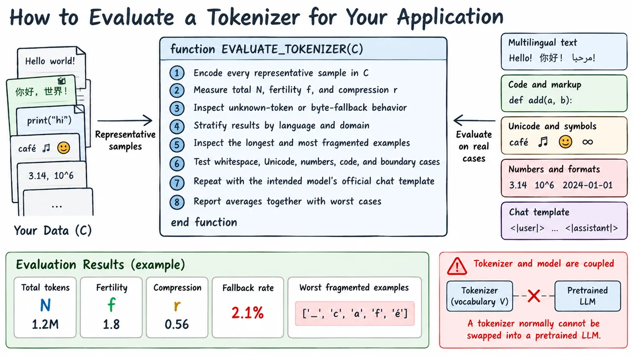
Once tokenization is treated as part of the deployed model rather than a generic text utility, evaluation becomes much more concrete. Start with a representative corpus built from the traffic you actually expect: the languages users write, the documents you retrieve, the code they paste, the JSON or Markdown your tools emit, and the kinds of long-tail strings that appear in production. A handful of clean English examples is not enough, because tokenizer weaknesses often live in the tails rather than the average case.
For every sample, record the total number of produced tokens . From the same corpus, calculate compression and fertility where a sensible word-like denominator exists. Then stratify those measurements. A single global mean can hide the fact that English prose is compact while Hindi text, source code, or long identifiers are much more fragmented. Report distributions by language and domain, not just one overall score.
Next, inspect the examples that produce the largest or strangest sequences. Sort samples by token count relative to source length and look at the worst cases directly. You want to know whether the tokenizer falls back to many tiny byte-derived pieces for rare Unicode, whether repeated whitespace explodes into extra positions, whether dates and decimals split awkwardly, and whether code identifiers or markup are unusually expensive. This is where the earlier edge cases become an engineering test suite rather than trivia.
Coverage deserves its own check. If the tokenizer has byte-level fallback, verify that unusual text remains reversible and observe how costly that fallback becomes. If the scheme can emit an unknown token, find out what kinds of inputs trigger it and whether distinct source strings collapse to the same unknown representation. A low unknown rate on ordinary prose is reassuring, but one unsupported character in a security-sensitive identifier or structured field can still matter.
For chat applications, repeat the measurement after applying the intended model's official conversation template. This often changes the result because system instructions, role markers, tool calls, separators, and end markers all add to the serialized sequence. The quantity that matters for context planning is the final model input, not merely the visible user text. If your application relies heavily on retrieval or tools, test those full flows as well.
A useful evaluation report should therefore contain at least these views: average and percentile token counts; and by language or domain; unknown or fallback behavior; examples with the worst fragmentation; and token counts after real chat serialization. If comparing several model-tokenizer pairs, run exactly the same corpus through each one so the differences are attributable to the interfaces rather than to different test data.
One final constraint changes how to act on the results. You usually cannot discover that another tokenizer is more efficient and simply plug it into an already pretrained LLM. The vocabulary , each , the embedding table , and typically the model's output layer were learned together. Swapping the tokenizer changes the meaning of the model's discrete interface. Making that swap generally requires substantial adaptation or retraining rather than a preprocessing configuration change.
So tokenizer evaluation has two different uses. When selecting among existing models, it helps you choose the model-tokenizer pair whose interface fits your workload. When designing a model from scratch, it informs the vocabulary and tokenizer you should train before the LLM learns around it. In both cases, the winning tokenizer is the one that behaves well on your real corpus and protocol—not the one that looks best on a generic benchmark sentence.
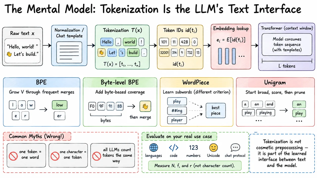
The most useful way to carry tokenization forward is as one end-to-end interface rather than a collection of isolated tricks. Start with the exact serialized input string . The tokenizer turns it into an ordered sequence of vocabulary entries, those entries become integer IDs, and the model uses the IDs to retrieve vectors from its learned embedding table:
The transformer never reads the original string directly. It receives the resulting sequence of learned vectors, and that sequence must fit—together with control/template tokens and generated output—inside the model's token limit .
Everything else in this article is about how that middle representation gets defined. BPE begins from small units and grows by repeatedly merging frequent adjacent pairs. Byte-level BPE moves the foundation down to UTF-8 bytes, giving arbitrary Unicode a fallback representation before larger merges are applied. WordPiece also learns reusable subwords but ranks candidate pieces differently from raw-frequency BPE. Unigram begins with many possible pieces, assigns them probabilities, compares whole segmentations, and prunes the vocabulary toward the target size.
Those algorithms do not operate in a vacuum. Corpus composition decides which patterns appear often enough to deserve compact representation. Normalization and pre-tokenization rules decide what the trainer sees. Whitespace, punctuation, code syntax, numbers, and Unicode structure can all move token boundaries. Special tokens and chat serialization add protocol-level structure that the user may never type explicitly. By the time a prompt reaches the transformer, tokenization has already made many decisions about how the text is presented to the model.
That is why three common intuitions should be discarded. One token is not one word. A token can be a word, part of a word, punctuation, whitespace-associated text, byte-derived material, or a control symbol. One character is not one token. A visible grapheme can contain several code points and bytes and can span several tokens. Different LLMs do not count the same text identically. Their vocabularies, preprocessing, training corpora, algorithms, and chat templates differ.
The operational consequences follow directly from this interface. Token count determines how much of the model's finite context budget is consumed. Fertility tells you how fragmented text is relative to chosen word-like units. Compression tells you how many source bytes each token represents on a corpus. Those quantities affect how much material fits into context and, in token-priced systems, can affect cost. They are useful engineering metrics, but none of them alone proves that one model is more capable than another.
So when evaluating a model for a real application, use the exact tokenizer and official chat template paired with that model. Measure representative languages and domains, then inspect the tails: rare Unicode, identifiers, long numbers, whitespace-heavy inputs, code, tool payloads, and adversarial boundary cases. A tokenizer that behaves well on generic English prose may still be inefficient where your application actually lives.
The final mental model is therefore simple but consequential: tokenization is not cosmetic preprocessing placed in front of an otherwise independent LLM. It is part of the learned contract between text and the model. The tokenizer decides the discrete symbols, the IDs give those symbols addresses, the embedding table gives those addresses learned vectors, and the model learns everything downstream assuming that interface will remain consistent.