Before we talk about attention, it is worth naming the problem it was designed to solve. A sequence model is not merely a machine that consumes tokens in order; it is a machine that must route information between positions. If token matters for predicting something at position , the architecture needs a reliable computational path from to . The central question is: how long, fragile, and sequential is that path?
Many important tasks can be written abstractly as sequence-to-sequence mappings,
where the input and output lengths may differ. Translation maps a sentence in one language to a sentence in another. Summarization maps a long document to a shorter text. Code generation maps a prompt or partial program to a completed program. Even when the output is not explicitly a separate sequence, language modeling has the same flavor: at each position , the model predicts the next token from the previous context,
This notation hides the hard part. The conditioning set may be large, but not every previous token is equally relevant. A model predicting the verb in a sentence may need to find the true subject many tokens earlier. A model completing code may need to remember an opening bracket, variable declaration, or function signature hundreds or thousands of tokens back. A translation model may need to align a word near the end of the source sentence with a word near the beginning of the target sentence. In all cases, sequence modeling requires selective communication between positions.
Classical recurrent neural networks handle this by passing information through a hidden state:
This is elegant because it respects temporal order and can in principle summarize everything seen so far. But it creates a narrow communication channel. If information from is needed at , it must survive repeated transformations through
The number of computational steps between the two positions grows with their distance, roughly . Gradients must also travel through this same chain during training. Gating mechanisms such as LSTMs and GRUs reduce the damage, but they do not remove the fundamental bottleneck: distant tokens communicate through a long sequential path.
Convolutional sequence models improve parallelism because all positions in a layer can be processed simultaneously. However, local convolutions have their own routing problem. A kernel of small width only mixes nearby tokens in one layer, so long-range interaction requires stacking many layers. Dilated convolutions shorten the path, but the architecture still imposes a predefined communication pattern. Whether two positions can exchange information efficiently depends on the convolutional design rather than on the content of the sequence itself.
This suggests three desiderata for a strong sequence architecture:
The key insight behind Transformers is to replace sequential recurrence with learned content-based communication. Instead of requiring information to move one step at a time through a hidden state chain, each position can directly ask: which other positions contain information useful for me? Attention implements this as a differentiable retrieval mechanism. Positions produce queries, keys, and values; similarity between queries and keys determines where information flows. The route is not hard-coded by distance or adjacency. It is learned from content.
This matters because many sequence dependencies are sparse but not local. A token may need its immediate neighbors for syntax, a faraway noun for agreement, and an even farther definition for semantic interpretation. Architectures based only on local or sequential propagation must repeatedly carry all potentially useful information forward. Attention instead allows the model to create direct edges between relevant positions, making the effective path length between and very short.
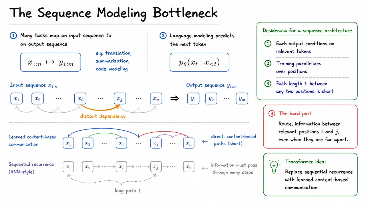
The visual below condenses this bottleneck into a single picture: an input sequence , an output sequence , and the central challenge of connecting distant but relevant positions. The faint recurrent chain represents the older strategy: information moves through many local transitions, producing a long path . The highlighted long-range arrow represents the dependency we actually care about.
The same visual also previews the Transformer solution. Rather than relying only on neighboring steps, positions exchange information through learned, content-based links. Those direct communication paths are the conceptual bridge from traditional sequence models to attention: the model still respects sequence structure, but it no longer forces all information to travel through a narrow sequential corridor.
The bottleneck is easiest to dismiss when we talk about it abstractly: “long-range dependency” sounds like a rare linguistic edge case. But the problem appears in one of the most ordinary tasks a language model performs: choosing the next word. Even a short sentence prefix can force the model to decide whether to trust nearby evidence or route information from a more distant but grammatically relevant token.
Consider the prefix
The next word should be “are”, not “is”:
The grammatical subject is keys, which is plural. But by the time the model reaches the prediction position, the most recent nouns are cabinet and door, both singular. A model that overweights local context may be tempted by the nearby phrase “near the door” and predict a singular verb:
This is the long-range agreement trap. The correct prediction depends not on the closest noun, but on the noun that structurally controls the verb. In the prefix,
is the controller, while
are distractors. The model must learn a conditional preference of the form
The important point is that this inequality is not merely about memorizing that “keys” often goes with “are.” It requires the model to identify which earlier token is relevant for this prediction. The phrase contains multiple nouns, and the nearest ones are misleading. Sequential distance and grammatical relevance have come apart.
This exposes a weakness of purely local prediction. If the model primarily summarizes recent tokens, then the final phrase “near the door” dominates the representation near the prediction point. But the word door should not control the verb. It is embedded inside a prepositional phrase modifying cabinet, which itself is embedded inside another prepositional phrase modifying keys. The relevant dependency skips over these intervening tokens.
A good sequence model therefore needs a mechanism for content-based routing. Instead of asking, “Which token is closest to the current position?”, it should ask something more like:
For subject–verb agreement, the feature being routed is number: plural versus singular. In other examples, it might be entity identity, coreference, topic, tense, quotation state, or a variable binding. The general pattern is the same: the model must retrieve information by relevance, not by position alone.
This is one of the motivations for attention. Attention will eventually give us a differentiable way to compare the current prediction context against earlier token representations and assign high weight to the tokens whose content matters. The long-range token does not need to be compressed through every intermediate step with equal fidelity; it can be selected directly when it becomes useful.
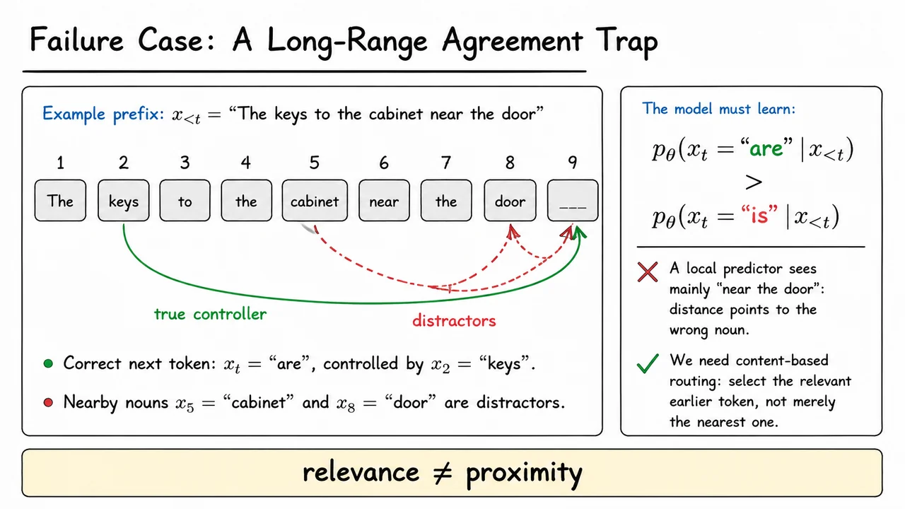
The visual below condenses this failure case into a single next-token decision. The prefix is laid out as token boxes, with the blank prediction position at the end. The plural noun keys is far away but is the true controller of the verb, while cabinet and door are closer distractors. The central mistake to avoid is treating proximity as a proxy for relevance.
The probability inequality on the right states the learning target: the model should assign higher probability to “are” than to “is” given the whole prefix. That small inequality captures the larger architectural lesson: long-range dependencies require mechanisms that can route information by content relevance, not merely by sequential neighborhood.
The agreement trap from the previous section is not just a quirky linguistic example; it exposes a more general systems problem. A model must move information from some earlier position —where the relevant subject, entity, or condition appears—to a later position , where that information is needed to make a prediction. The intervening tokens may be syntactically plausible distractors, but semantically irrelevant. The question is: how many computational steps must the signal traverse before position can use what position knew?
For a recurrent model, the route is built into the architecture. Information at is first absorbed into a hidden state , then passed forward one position at a time:
This gives RNNs a useful inductive bias: nearby temporal continuity is natural, and the hidden state acts like a running summary. But the same design becomes a bottleneck for long-range dependencies. If and are far apart, then the representation of must survive many state updates, each of which may overwrite, compress, or distort it. Even if the model has gates, such as in an LSTM or GRU, the route is still sequential. The architecture can learn to preserve information, but it cannot avoid the fact that the information must pass through many intermediate states.
The training signal suffers from the same geometry. When a loss at position assigns credit to something that happened near , the relevant derivative contains a long product of Jacobians:
This product is the mathematical heart of the vanishing and exploding gradient problem. If the typical singular values of these Jacobians are smaller than one, the gradient decays exponentially with distance; if they are larger than one, it can blow up. Gating, normalization, careful initialization, and gradient clipping can make this more manageable, but they do not remove the long credit-assignment path. The model is still being asked to propagate both information and gradients through sequential transformations.
Convolutional sequence models attack the problem differently. Instead of carrying a hidden state from left to right, they update all positions in parallel using local windows. This is excellent for parallel training: every position in a layer can be computed at the same time. But locality introduces a different limitation. A token can only influence positions within the receptive field of the convolution, and that receptive field grows layer by layer. With a kernel of fixed width, distant positions require many layers before they can interact.
So CNNs trade the RNN’s sequential time bottleneck for a depth bottleneck. A sufficiently deep convolutional network can connect distant positions, and dilated convolutions can expand the receptive field faster, but the architecture still imposes a structured route through intermediate neighborhoods. Distant communication is possible only after repeated mixing. In practice, this means either many layers, large kernels, carefully chosen dilation schedules, or some combination of these. The model’s ability to relate and is mediated by architectural distance.
This is the motivation for attention as a new primitive. Instead of forcing information to travel through every intermediate hidden state, or to diffuse through local convolutional neighborhoods, we would like position to directly retrieve information from position when is relevant. In the idealized path-length sense, attention offers:
That statement does not mean attention is computationally free. Full self-attention over a sequence of length compares many pairs of positions, which introduces its own cost. Rather, the point is about communication distance: once the attention scores are computed, any position can incorporate information from any other position in a single layer. The burden shifts from “can the information survive the route?” to “can the model learn which positions matter?”
This shift is subtle but crucial. RNNs and CNNs bake in a strong notion of locality: information moves through adjacent time steps or nearby windows. Attention weakens that assumption and replaces it with content-based routing. If a verb at position needs the subject at position , the model can learn to assign high weight to that subject directly, even across many distractors. The resulting architecture is often easier to optimize for long-range dependencies because the forward information path and the backward credit-assignment path are both shorter.
The comparison can be summarized as follows:
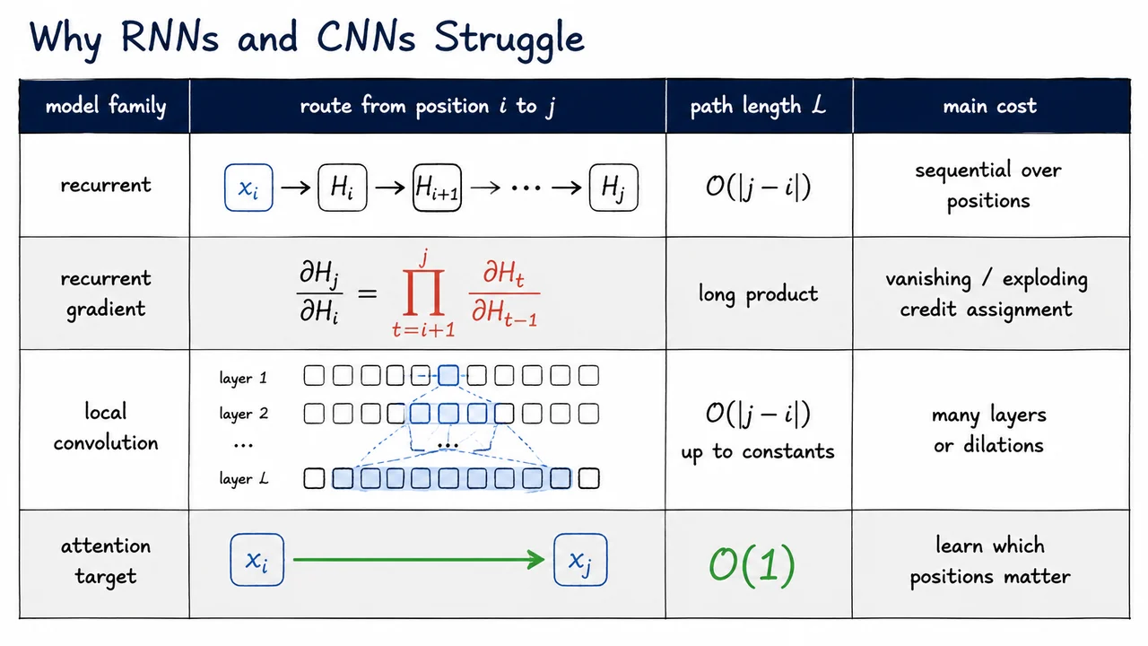
The visual below condenses this argument into a side-by-side comparison. The recurrent row emphasizes the chain from to , while the gradient row highlights why that chain is also an optimization problem. The convolutional row captures receptive-field growth through stacked local windows. The attention row contrasts these with a direct connection from to , foregrounding the key design goal: reduce the path length for relevant interactions to .
Read the table not as saying that attention is universally cheaper or always better, but as isolating the architectural reason Transformers became compelling. They replace forced sequential or local communication with a differentiable mechanism for deciding who should talk to whom. That mechanism—attention as learned lookup—is the next object we will derive.
The previous discussion identified a common bottleneck behind both recurrence and convolution: routing information. If a token near the end of a sequence needs evidence from a token near the beginning, an RNN must carry that evidence through many recurrent steps, while a CNN must propagate it through many local receptive fields unless the network is made very deep or uses large kernels. The issue is not merely that long paths are inconvenient; long paths make learning fragile. Gradients, intermediate states, and local transformations all become part of the communication channel.
A more direct primitive would let each position ask: which other positions contain information useful for me right now? Instead of forcing information to move step by step through a fixed computational graph, we want every position to be able to retrieve relevant content from anywhere in the sequence in one operation. This is the motivation behind attention.
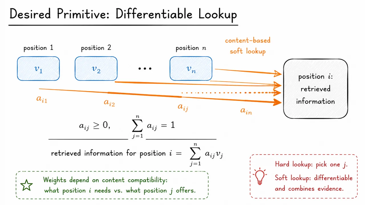
The simplest abstraction is a content-based lookup. Imagine that each position in a sequence stores some information in a vector , called a value vector. Now suppose position wants to update its representation. Rather than reading only its neighbor or the previous hidden state, position forms a weighted combination of all available values:
The coefficients are the attention weights. They say how much position retrieves from position . To make this retrieval behave like a soft selection, the weights are constrained to be nonnegative and sum to one:
These constraints make the retrieved vector a convex combination of the value vectors. Intuitively, position is not copying a single source exactly; it is averaging information from multiple sources, with more relevant positions receiving larger weights. This convex-mixture view is important because it gives attention a stable numerical interpretation: the output remains in the span of available information rather than becoming an unconstrained linear explosion.
A hard lookup would choose one position and return . That is useful in classical data structures, but it is awkward for gradient-based learning: a discrete choice is not smoothly differentiable with respect to the scores that produced it. Attention replaces that hard decision with a soft lookup. If the model is uncertain between two relevant tokens, it can assign weight to both. If training later reveals that one source was more useful, gradients can continuously shift probability mass toward it.
This also explains why attention is more than a memory trick. The weights should not be fixed by distance or position alone. They should depend on content compatibility: what the current position needs and what each candidate source offers. For example, in a translation model, a decoder position producing a verb may need to retrieve the subject from far away. In a language model, a pronoun may need to retrieve a compatible antecedent. The useful source is determined by meaning and context, not simply by being nearby.
There are a few subtle assumptions hidden in this primitive. First, the value vectors must contain information worth retrieving; attention can route information, but it cannot recover content that was never represented. Second, the weights must be produced by a learnable scoring mechanism that can compare position 's needs with position 's contents. Third, because the retrieved vector is a mixture, attention can sometimes blur information when many incompatible sources receive nontrivial weight. Later, scaled dot-product attention will address how to compute these weights effectively and how to keep the scoring distribution numerically well behaved.
The key conceptual shift is therefore:
The visual below condenses this idea into a single routing picture. The sequence positions each hold a value vector . For a target position , arrows from all positions represent possible communication channels, and their thickness represents the learned attention weights . The output at position is not one copied vector, but the soft mixture .
This compact diagram is the bridge from motivation to mechanism. We have not yet specified how the weights are computed—that will require embeddings, queries, keys, values, and scaling—but we have specified the primitive we want: differentiable, content-based retrieval over a sequence.
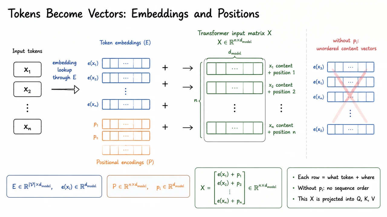
Now that we have framed attention as a kind of differentiable lookup, we need to answer a deceptively basic question: what exactly are we looking up with? A Transformer cannot operate directly on raw symbols like "cat", "sat", or ".". Those symbols are discrete vocabulary items; they have no geometry, no dot products, no notion of similarity that a neural network can manipulate smoothly. Before attention can compare one token to another, every token must be represented as a vector in a shared continuous space.
The first ingredient is the token embedding table. If the vocabulary is and the model width is , we learn a matrix
Each row of is the learned vector representation of one vocabulary item. For a token , the embedding lookup returns
This is often described as a “lookup,” but it is still part of the differentiable model: the selected embedding vector participates in the forward computation, receives gradients during backpropagation, and is updated during training. Over time, the model learns an embedding geometry in which useful distinctions for prediction become linearly accessible to later layers.
However, token identity alone is not enough. The sequence
does not mean the same thing as
If we gave self-attention only the multiset of token embeddings , then the model would know which tokens appeared, but not where they appeared. This is especially important because vanilla self-attention, unlike recurrence or convolution, does not inherently process tokens left-to-right or through local neighborhoods. Its core operation compares rows of a matrix to other rows of the same matrix. Without additional positional information, that operation is naturally permutation-equivariant: reorder the input rows, and the corresponding outputs reorder in the same way.
So Transformers add a second vector to each token representation: a position vector. For a maximum sequence length , we can represent these position vectors as rows of a matrix
The vector tells the model that this row corresponds to position . In the original Transformer, these were sinusoidal encodings; in many modern models, they are learned or replaced with relative/rotary variants. But the conceptual role is the same: position information must enter the representation somehow, because attention by itself only sees a set of content vectors.
The simplest absolute-position construction is additive. For each token , we combine “what token is here” with “where it is”:
Stacking these row vectors gives the Transformer’s input matrix
This matrix is the object that will be projected into queries, keys, and values in the next step. Each row is one token position, and each row lives in the same -dimensional space.
The addition is worth pausing over. We are not concatenating token and position into a larger vector; we are superimposing them in the same model dimension. That means the model must learn to use the shared coordinates to encode both lexical/content information and positional information. This works because the subsequent linear projections can learn directions that respond to content, position, or mixtures of the two. But it also encodes an assumption: the model width must be large enough to carry all the information the network needs.
A useful way to think about a row of is:
That last phrase is crucial. Attention will not retrieve information from isolated word types; it will retrieve from contextualizable slots in a sequence. The same token can appear in two positions and begin with the same embedding, but after adding different 's, the initial vectors are no longer identical. This allows later attention layers to distinguish, for example, the first occurrence of a word from the second.
There is also an important failure mode hiding here. If we omitted , then a self-attention layer with shared projections would not know whether a token came first, last, or somewhere in the middle. It could still compare content, but it would lack sequence order. For tasks where order matters—and almost all language tasks do—that is a severe limitation. Positional information is therefore not a decorative add-on; it is what turns a bag of token vectors into a sequence representation.
The visual below compactly summarizes this construction as a pipeline: raw tokens are mapped through the embedding table , position rows are supplied from , and corresponding vectors are added row by row to form . The key idea to look for is that the Transformer input is not “just embeddings,” but embeddings plus positions.
It also foreshadows the next step. Once has been assembled, attention can create queries, keys, and values by learned linear projections. In other words, the differentiable retrieval mechanism we want is built on top of this matrix: each row of is now a content-and-position-aware record that attention can compare, weight, and combine.
Once tokens have been turned into vectors, we have a useful representation at every sequence position—but each position is still mostly carrying local information: “what token am I?” and “where am I?” The next problem is how one position can use information stored at other positions. If the word “it” appears late in a sentence, its representation may need to borrow meaning from a noun many tokens earlier. If a code variable is used after several lines, its current representation should be able to retrieve the earlier definition.
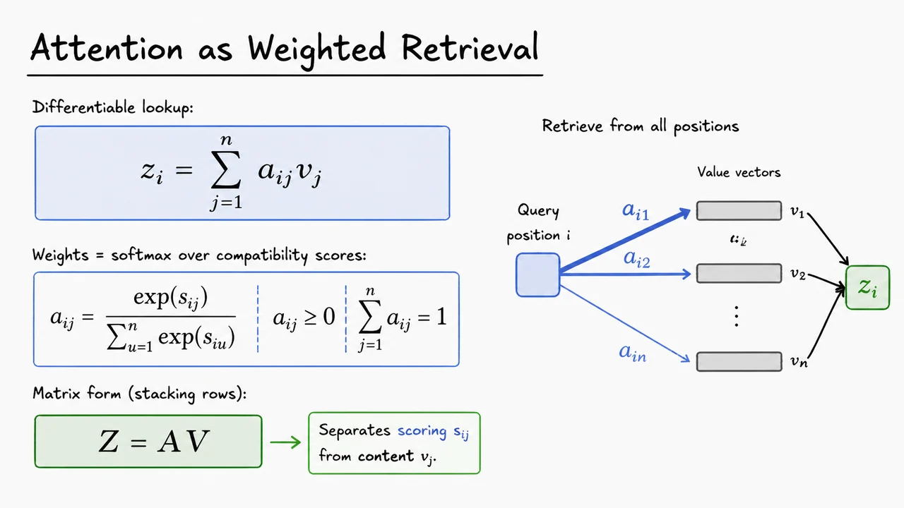
The key idea of attention is to make this retrieval differentiable. Instead of choosing exactly one previous token or one memory slot, a position forms a weighted average over many stored vectors. For a particular query position , suppose every position stores some vector , called a value. The output representation at position is
This is the central retrieval equation. The output is not copied from a single location; it is blended from all available values. The coefficient tells us how much position retrieves from position .
For this weighted average to behave like retrieval, the weights should be nonnegative and should sum to one:
So lies in the convex hull of the value vectors. Intuitively, attention says: “construct the new representation by mixing stored content, with mixture proportions determined by relevance.” This is a softer and more trainable version of lookup in a dictionary or memory table.
The weights themselves come from compatibility scores , where measures how relevant position is to position . We convert these arbitrary real-valued scores into normalized weights using a softmax over the retrievable positions:
The denominator is important: for a fixed retrieving position , the model compares all candidate positions against one another. Attention is therefore relative: a token receives high weight not merely because its score is large in isolation, but because its score is large compared with the alternatives in the same row.
This row-wise normalization has several consequences. First, attention weights are easy to interpret as a distribution over source positions. Second, the operation is differentiable end-to-end, so learning can adjust both the scoring mechanism and the stored value vectors. Third, the softmax introduces competition: increasing tends to decrease the mass assigned elsewhere. That competition is part of what makes attention behave like selective retrieval rather than an unstructured sum.
There is also a subtle but crucial separation here: scoring and content are conceptually different. The score determines where to look; the value determines what information is retrieved once we look there. This distinction will become central when we introduce queries, keys, and values. For now, it is enough to notice that the vector used to decide relevance need not be identical to the vector whose information is ultimately copied into the output.
Stacking the outputs for all positions gives the matrix form. Let contain the value vectors row by row, and let contain the attention weights, with row holding the distribution . Then
This equation is compact but powerful. Each row of is a weighted average of the rows of . The matrix is not just a generic linear map; it is row-stochastic, meaning each row is a probability distribution. Attention is therefore a structured, data-dependent linear combination of stored representations.
The visual below condenses this idea into two complementary views. On the algebraic side, it emphasizes the chain from scores , to softmax-normalized weights , to retrieved output . On the retrieval side, one position sends different-strength connections to several stored values , and those weighted contributions merge into the output vector.
The most important takeaway is that attention is not yet “magic Transformer machinery.” At this stage, it is simply weighted differentiable retrieval. The model computes relevance scores, normalizes them into a distribution, and uses that distribution to average content vectors. The next step is to specify how the scores are produced—and that is where queries, keys, and values enter.
The weighted-retrieval view gives us a useful abstraction: once we have an attention matrix , producing outputs is just
a weighted average of “retrievable” vectors. But this leaves an important question unresolved: where do the weights in come from, and what exactly are we averaging? If the same representation of a token is used both to decide whether it is relevant and to supply the content returned, the model is forced to entangle two different roles. Transformers avoid this by separating matching from retrieval.
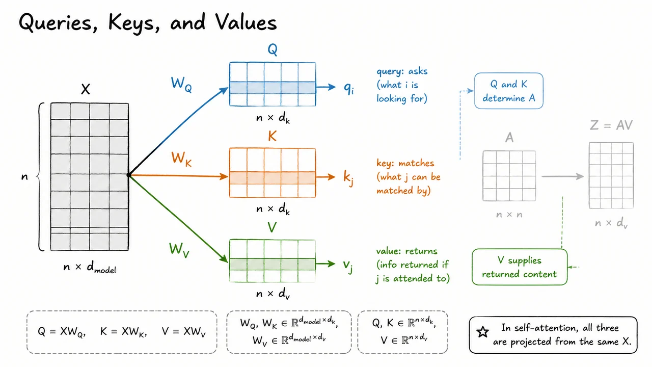
The key move is to project each input position into three learned spaces:
Here is the sequence of contextual token representations: positions, each represented by a -dimensional vector. The learned projection matrices have shapes
so the resulting matrices are
Conceptually, each row of these matrices plays a different role. The row of is the query for position : it represents what that position is looking for. The row of is the key for position : it represents how position advertises itself for matching. The row of is the value for position : it is the information returned if some other position decides to attend to .
This distinction is subtle but central. A word may need to be matched according to one set of features, while returning a different set of features once selected. For example, a pronoun might look for a compatible noun phrase using syntactic and semantic cues encoded in queries and keys, but the information retrieved from the noun phrase might include number, gender, entity identity, or broader contextual meaning encoded in the value vector. The model should not have to use the same coordinates for all of these purposes.
In self-attention, all three matrices are projected from the same input . That is why the mechanism is “self”: every position can attend to other positions in the same sequence. But the projections are different, so “same source” does not mean “same representation.” The model learns three views of each token:
This separation also explains why attention is more flexible than a fixed similarity computation on raw embeddings. If we compared rows of directly, the notion of relevance would be tied to whatever features happen to be present in the model representation. By learning and , the Transformer learns a task-specific compatibility space. By learning , it separately learns what content should flow forward after compatibility has been determined.
There are also important dimensional choices hidden in these equations. The query and key dimensions must match, because they will be compared to produce attention scores; hence both live in . The value dimension , however, need not equal , because values are not used for matching in the same way. They are aggregated after the attention weights have already been computed. In practice, architectures often choose convenient equal dimensions, especially inside multi-head attention, but the mathematical roles remain distinct.
A useful way to think about the full computation is:
So and answer the question, “Which positions should interact, and how strongly?” while answers, “What information should be passed along once that interaction is chosen?” This is the bridge from abstract weighted retrieval to the concrete attention mechanism used in Transformers.
The visual below compactly summarizes this decomposition. A single input matrix branches into three learned projections: , , and . The parallel arrows emphasize that these are not three different input sequences, but three learned views of the same sequence. Highlighting individual rows , , and reinforces the position-wise interpretation: one position asks, another position matches, and the matched position returns content.
The faded continuation toward is also important. It reminds us that values are still the objects being averaged, as in weighted retrieval, but the weights will now be produced by comparing queries and keys. This separation is the conceptual step that makes scaled dot-product attention possible: first learn what to match, then learn what to return.
With queries, keys, and values in place, the next question is: how should a query decide which keys are relevant? We have already separated “what I am looking for” () from “what each position offers as an address” () and “what content I can retrieve” (). Attention now needs a compatibility function that turns each query–key pair into a scalar score.
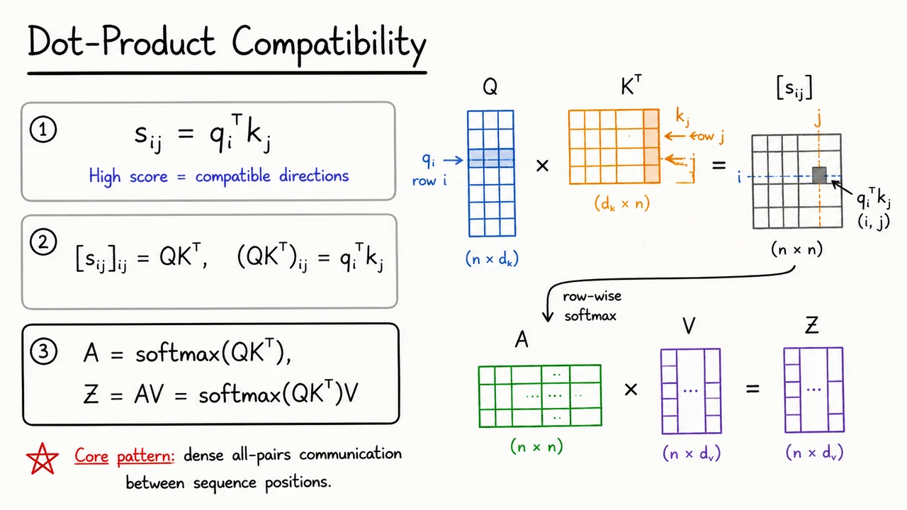
The simplest and most important choice is the dot product:
This score is large when and point in compatible directions. Geometrically, the dot product rewards alignment: if two vectors have similar directions, their inner product is positive and large; if they are orthogonal, it is near zero; if they point in opposing directions, it can be negative. In attention, this means position assigns a high raw score to position when the learned query at matches the learned key at .
There is a subtle but important assumption here: the learned projections that produce and are free to shape the space in which “matching” happens. We are not comparing raw token embeddings directly. Instead, the model learns a coordinate system where certain directions correspond to useful retrieval patterns: syntactic agreement, coreference, local continuation, delimiter matching, or any other relation that helps the task. The dot product is simple, but the learned projections make it expressive.
For a sequence of length , every query position compares itself to every key position. If we stack the query vectors into a matrix
and the key vectors into
then all pairwise dot products appear at once in the matrix product
This is one of the central computational facts behind Transformers: attention is vectorized all-pairs comparison. Instead of iterating through the sequence recurrently, each position can compare against every other position in a single batched matrix multiplication. That is why attention is so well matched to modern accelerators: the communication pattern is dense, but it is expressed as large linear algebra operations.
The raw score matrix is not yet a retrieval distribution. Each row contains the scores for one query position against all possible source positions . To turn these scores into weights, we apply a row-wise softmax:
Here can be read as “how much position attends to position .” The rows of sum to one, so each query forms a weighted average over values. The retrieved output vectors are then
This is the full dot-product attention pattern before scaling and masking: compare queries to keys, normalize scores into attention weights, then use those weights to average values.
It is worth emphasizing what this buys us. A recurrent model must pass information through a chain of hidden states, so distant positions interact through many sequential steps. A convolutional model needs either large kernels or many layers to connect distant tokens. Dot-product attention, by contrast, gives every position a direct path to every other position in one layer. The cost is that the score matrix has entries, so dense self-attention is powerful but expensive for long sequences.
There are also important failure modes hidden in this compact formula:
The next section will address the first of these issues directly: why the raw dot product is divided by . For now, the key idea is that dot-product attention is not mysterious. It is a learned content-addressable lookup system implemented as matrix multiplication.
The visual below consolidates this flow. On the left, the equations isolate the three conceptual steps: define a pairwise compatibility score, vectorize all scores as , and retrieve values using softmax-normalized weights. On the right, the matrix pipeline makes the same idea operational: rows of meet rows of through , producing a score grid whose cell is exactly .
The important thing to notice is the dense all-pairs communication pattern. Every query row has access to every key column before the softmax chooses how much value information to retrieve. That single pattern,
is the algebraic heart of attention.
Having introduced dot products as a natural compatibility score between a query and a key, there is one more detail that looks like a harmless implementation trick but is actually crucial for stable learning: Transformer attention does not use directly. It uses a scaled dot product.
The raw score between query and key is
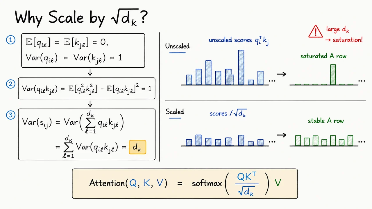
At first glance, this seems perfectly reasonable. If the query and key point in similar directions, the dot product is large; if they are unrelated or opposed, it is small or negative. But the magnitude of this score depends not only on semantic alignment. It also depends on the key/query dimension . As grows, the dot product accumulates more random terms, so even unrelated vectors can produce scores with increasingly large variance.
A simple initialization-style calculation makes the issue visible. Suppose the components of and are independent, centered, and normalized:
These assumptions are not meant to describe every trained Transformer exactly. They are a controlled approximation: before learning has shaped the representations too much, and under common normalization/initialization schemes, it is reasonable to ask what scale the scores would have if the components behaved like independent unit-variance random variables. The goal is to prevent the architecture itself from injecting an undesirable scale factor.
For one coordinate product, independence gives
and
So each coordinate contributes a unit-variance random term to the dot product. Since the full score sums such terms, the variance grows linearly:
Equivalently, the standard deviation of the raw dot product grows like . This is the key point: increasing the representation dimension makes the scores larger in magnitude even when there is no stronger evidence of relevance.
That matters because attention does not use the scores directly; it passes them through a softmax. The softmax is sensitive to scale. If its inputs are small or moderate, it can assign a graded distribution over many keys. But if one logit is much larger than the others, the output becomes nearly one-hot:
Large score variance therefore pushes attention into a saturated regime. One key receives almost all the probability mass, the others receive almost none, and the gradients through the softmax become less informative. The model may still train, but optimization becomes unnecessarily brittle: early random score differences can dominate attention before the network has learned meaningful retrieval patterns.
The fix is to normalize the score by its typical standard deviation. Since
we compute attention using
This does not change the basic content-based retrieval story. Queries still compare themselves to keys, and values are still averaged according to the resulting attention weights. The scaling only keeps the logits in a numerically and statistically reasonable range as the key/query dimension changes.
A useful way to read the result is:
The visual below condenses this argument into two complementary views. On one side, the variance derivation tracks how the score accumulates independent unit-variance products, ending in the highlighted conclusion . On the other side, the same phenomenon is shown operationally: unscaled scores become tall and uneven, producing a sharply peaked attention row, while scaled scores produce a smoother, more stable distribution.
The important takeaway is not that attention should always be diffuse. A trained Transformer can and often should place highly concentrated attention when the data calls for it. The point is that this concentration should be learned, not forced by the dimensionality of the dot product. Scaling by makes dot-product attention behave consistently across dimensions, giving the softmax a well-conditioned set of logits to work with.
After controlling the scale of the dot products, the next issue is not how strongly one token should attend to another, but whether that link should exist at all. Attention, by default, is completely content-driven: every query compares itself with every key, and the softmax turns those comparisons into a probability distribution over all value vectors. That is powerful, but it is also too permissive. Some attention links are structurally invalid regardless of content.
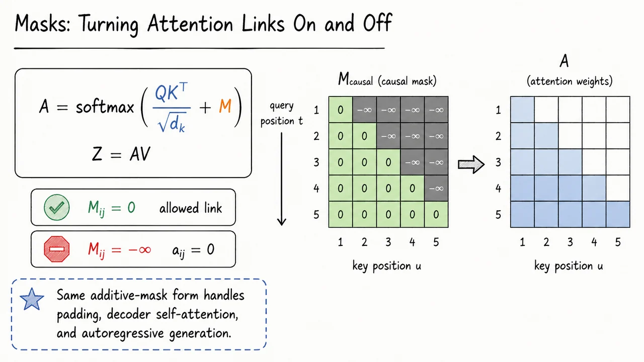
The mechanism for enforcing these hard constraints is an attention mask. Starting from the scaled attention logits,
we add a mask matrix before applying the row-wise softmax:
Here has the same row-column structure as the attention score matrix: rows correspond to query positions, columns correspond to key/value positions. The key idea is that masking happens at the logit level, before normalization. This matters because the softmax is sensitive to additive changes in logits: setting a logit to makes its exponent exactly zero.
Concretely, for query position and key/value position ,
means the link is allowed. The original scaled dot-product score is unchanged, so the model may assign attention mass to if the content match is strong. In contrast,
means the link is forbidden. Since
the corresponding softmax weight becomes
Therefore contributes nothing to the output vector at query position , no matter how compatible and might have been.
This is a hard structural constraint, not a learned preference. The model is not being encouraged to avoid certain links; it is made mathematically impossible for those links to carry information. In actual implementations, is often represented by a very large negative number for numerical reasons, but the intended operation is the same: after softmax, the masked probability is zero or effectively zero.
The most important example is causal self-attention, used in autoregressive language modeling. When predicting token , the model may use tokens at positions , but it must not look ahead to future positions . Otherwise, training would leak the answer: the representation for an earlier token could directly depend on later tokens that should not yet be known during generation.
The causal mask is therefore
This gives a lower-triangular pattern, including the diagonal. Position can attend only to itself, position can attend to positions and , and so on. The diagonal is usually allowed because the representation at a position may use the token currently being processed when computing hidden states for next-token prediction; what is forbidden is access to future positions.
The same additive-mask abstraction covers several different situations:
A subtle but important point is that masks operate independently of the learned parameters. The matrices , , and are still produced by learned projections, and the model still decides among allowed links using content similarity. The mask simply defines the set of possible routes through which information may flow. In graph terms, attention learns edge weights, while the mask determines which edges are present.
The visual below condenses this into two complementary views. On the left, the mask appears exactly where it belongs mathematically: added to the scaled dot-product logits before the softmax. The two cases and then become easy to interpret as “keep this candidate link” versus “force its attention weight to zero.”
On the right, the causal mask is represented as a triangular matrix. The allowed region contains zeros, while the forbidden future region contains . After the row-wise softmax, that forbidden upper triangle disappears from the attention matrix : future value vectors cannot contribute to earlier query positions. This is the small algebraic trick that makes Transformer attention compatible with autoregressive sequence modeling.
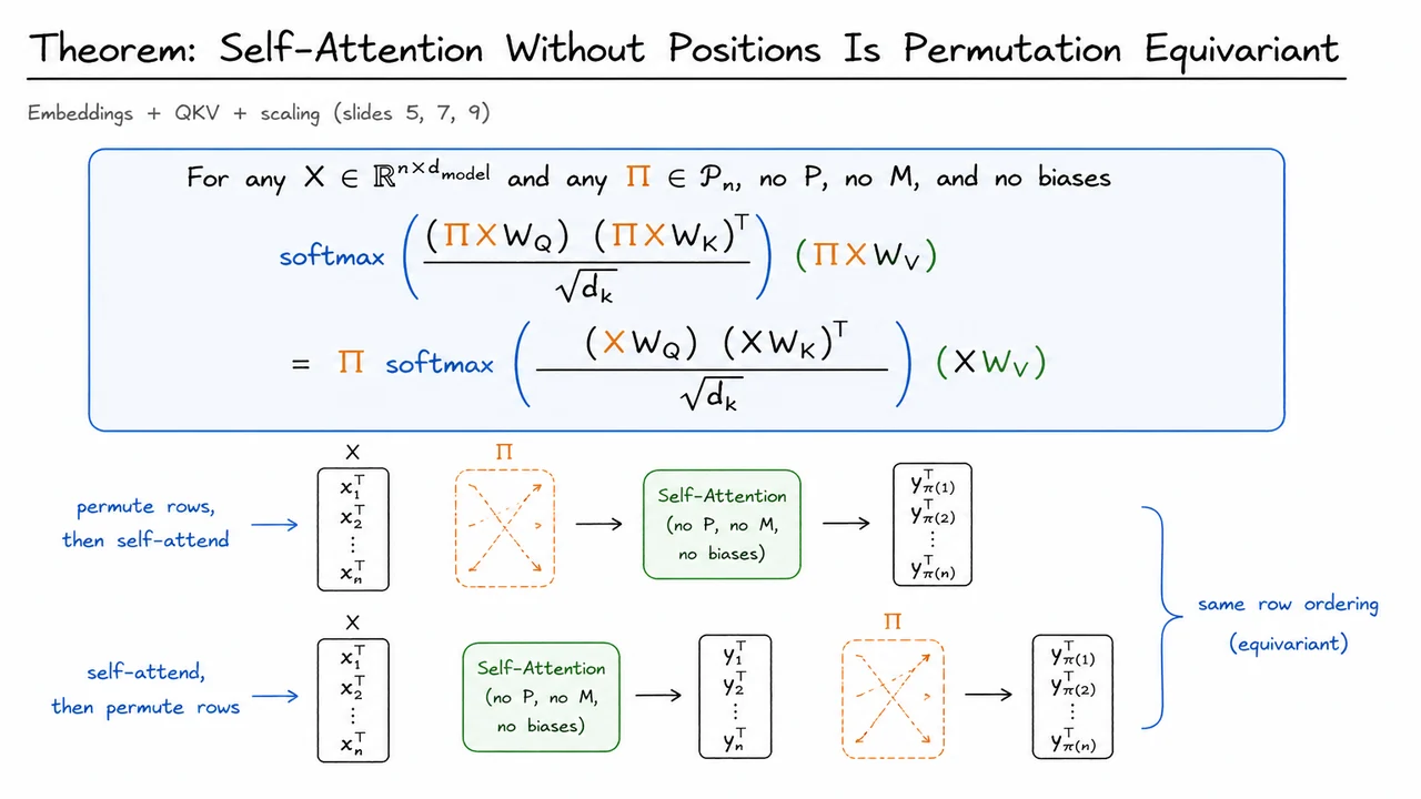
After introducing masks, it is tempting to think of attention as a graph over sequence positions: some token positions may attend to others, and masking removes selected edges. But before we add masks—or positional encodings—there is a deeper fact hiding in plain sight: content-only self-attention does not know what a sequence order is. It sees an matrix as a collection of row vectors and computes interactions among those rows, but nothing in the vanilla attention formula says that row comes before row , or that row is special because it is first.
Let , where each row is a token representation. A single-head self-attention layer without positional information computes
and then
The softmax is applied row-wise: each query row produces a probability distribution over all key rows, and then forms a weighted average of value rows. This is content-based retrieval: each token asks, “which other token vectors are relevant to me?” The important subtlety is that relevance is computed only through dot products of learned projections. There is no term involving the integer index , no sinusoidal or learned positional vector , and no causal or padding mask that distinguishes allowed from disallowed positions.
Now consider a permutation matrix . Multiplying on the left by simply reorders the rows of . For example, if contains token vectors in one order, then contains the same token vectors in a different order. The theorem says that self-attention commutes with this reordering:
That property is called permutation equivariance. It is not invariance: the output does change when the input is permuted. But it changes in exactly the same way—the output rows are permuted by the same . In other words, content-only self-attention treats the input as an unordered set of token vectors, while still returning one output vector per input token.
The algebra is short but instructive. If we permute the input rows, the projected queries, keys, and values become
The new attention score matrix is
So the score matrix is not arbitrary; it is the original score matrix with both rows and columns permuted. Rows are permuted because the queries have been reordered, and columns are permuted because the keys have been reordered. The scaling by does not affect this symmetry.
The only slightly delicate step is the row-wise softmax. For any score matrix ,
This holds because permuting a row before applying softmax simply permutes the resulting probabilities in the same way, and permuting the collection of rows also just reorders the row-wise outputs. Applying this to
we get
Multiplying by the permuted values cancels the inner permutation:
Substituting back , , and , the theorem is exactly
This result matters because language is not merely a bag of token embeddings. The sentences “dog bites man” and “man bites dog” contain the same token set but mean different things. A Transformer without positional information cannot distinguish these two sequences by order alone. If the token embeddings are identical and only their rows are rearranged, the layer can only rearrange its outputs correspondingly. It has no intrinsic mechanism for representing “before,” “after,” “nearby,” or “first.”
There are also useful boundary cases to keep in mind. The equivariance statement assumes no positional encoding , no mask , and no position-dependent biases. Adding absolute positional embeddings breaks the symmetry because row receives information tied to index . Adding a causal mask also breaks full permutation equivariance because the mask privileges the left-to-right order. By contrast, operations applied identically to every row—such as a shared feed-forward network, residual addition, or layer normalization over features—typically preserve permutation equivariance. The symmetry is broken only when the model is given some information that distinguishes positions.
The visual below compactly summarizes the theorem as a commuting diagram: one path permutes the input rows first and then applies self-attention, while the other applies self-attention first and then permutes the output rows. The equality says these paths arrive at the same result. That is the operational meaning of permutation equivariance.
The equation in the theorem box is the algebraic version of the same story. The orange terms track row permutations, the blue softmax block tracks how attention weights reorder consistently, and the green value block reminds us that the final weighted sums are attached to the same permuted rows. The important takeaway is simple but profound: without positions or masks, self-attention is a powerful content-retrieval mechanism, but not yet a sequence model in the ordered sense.
The equivariance result is useful precisely because it tells us what self-attention cannot know by itself. If the inputs are just token embeddings, self-attention treats the sequence as a set of content vectors with indices attached only externally. It can route information based on what appears, but not intrinsically on where it appears. That is elegant from a symmetry perspective, but disastrous for language, programs, music, genomes, and essentially every sequence domain where order changes meaning.
For example, the two strings “the dog bit the man” and “the man bit the dog” contain almost the same multiset of token identities. A content-only self-attention layer can produce correspondingly permuted representations, but it has no built-in reason to distinguish subject position from object position. The problem is not that attention is weak; the problem is that attention is too symmetric. We must deliberately break permutation symmetry by injecting positional information.
The standard Transformer does this by replacing each token embedding with a position-aware input representation such as
where is a vector associated with position . Now the attention mechanism no longer receives just “the embedding for this word”; it receives “the embedding for this word at this location.” The dot products used to compute attention can depend on token identity, position, and interactions between the two. In other words, attention remains content-based retrieval, but the content being retrieved has been enriched with location.
There are several ways to choose the positional signal. The original Transformer used sinusoidal positional encodings, where each coordinate varies periodically with position at a different frequency. Learned absolute embeddings are also common: the model simply learns a table . More recent architectures often use relative position biases or rotary positional embeddings, which modify the attention scores or query/key geometry so that the model reasons more directly about offsets like “three tokens ago” rather than absolute coordinates like “position 57.”
These choices differ in what generalization they encourage:
A subtle point is that masking is not a full substitute for positional encoding. A causal mask does introduce an ordering constraint: token cannot attend to future tokens . But without positional information, the model still has limited ability to distinguish different permutations of the visible prefix. The mask says “you may look backward,” but it does not fully tell the model which earlier token was first, second, or adjacent in a content-independent way. For sequence modeling, causality and position solve different problems: causality prevents information leakage, while positional encoding gives the model a coordinate system.
This also explains why positional information matters even in encoder-only models, where there is no causal mask. In a bidirectional encoder, every token can attend to every other token. Without positions, the representation of a sentence is equivariant to arbitrary reordering. A downstream classifier might collapse those token representations into something nearly permutation-invariant, making word order even harder to recover. Positional encodings give the encoder a way to represent syntactic roles, local neighborhoods, phrase boundaries, and long-range dependencies as structured relations rather than unordered co-occurrences.
The visual summary for this idea should be read as a symmetry-breaking story: content-only self-attention preserves permutation structure, while adding positional signals turns a bag-like collection of embeddings into an ordered sequence. Once token and position information are combined, attention can still retrieve by similarity, but similarity is now computed in a space where “same word in a different place” can mean something different.
This sets up the next architectural refinement. After we give the model a notion of position, a single attention operation still represents only one retrieval pattern at a time. In practice, different relationships matter simultaneously: nearby syntax, long-range agreement, delimiter matching, coreference, copying, and positional offsets. Multi-head attention will let the model learn several such retrieval subspaces in parallel.
Before assembling a full Transformer block, it is worth pausing on the attention mechanism itself. A single scaled dot-product attention layer already gives us a powerful content-addressable retrieval operation: each token forms a query, compares it against all keys, and uses the resulting weights to average the corresponding values. But one attention distribution is still only one way of asking, “What information should this token retrieve from the sequence?”
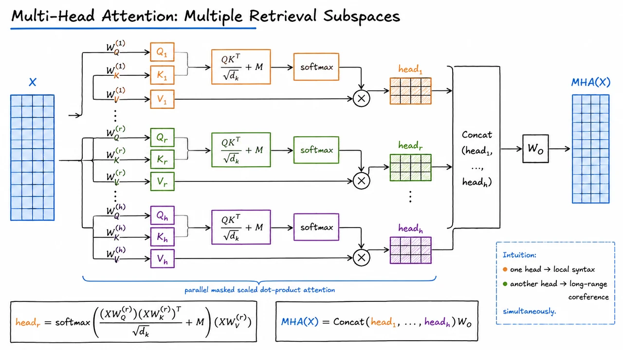
The central idea of multi-head attention is that a token may need to retrieve several different kinds of evidence at once. In language, for example, a word might need nearby syntactic context, a long-range subject for agreement, a previous mention for coreference, and a delimiter or boundary token for structure. These are not necessarily well represented by a single similarity function over one query-key space. Multi-head attention addresses this by running several attention mechanisms in parallel, each with its own learned projections.
Given an input sequence representation , each head learns separate projection matrices
These produce head-specific queries, keys, and values:
The head then performs the same scaled dot-product attention operation we have already developed:
The mask plays the same role as before: it can forbid attention to certain positions, such as future tokens in causal decoding or padding tokens in batched training. The scaling by also remains essential, because each head computes dot products in its own key/query dimension . Without scaling, the logits can grow too large in magnitude as increases, causing the softmax to become overly peaked and gradients to become less useful.
The important change is not the formula inside one head; it is the fact that each head has its own learned retrieval subspace. One head might learn projections where query-key similarity emphasizes syntactic adjacency. Another might emphasize semantic similarity. Another might specialize in positional or delimiter-like patterns. This specialization is not manually assigned; it emerges because the model can reduce training loss by distributing different retrieval behaviors across heads.
After computing all heads in parallel, their outputs are concatenated:
This concatenated representation contains multiple retrieved views of the sequence at each token position. A final learned output projection then mixes these views back into the model dimension:
This final projection is easy to underestimate. Concatenation alone would merely place the heads side by side. The output matrix lets the model form learned combinations across heads: it can amplify, suppress, or blend information retrieved by different attention patterns. In other words, multi-head attention is not just “several attentions in parallel”; it is parallel retrieval followed by a learned recombination step.
A common implementation choice is to keep the total compute roughly comparable to a single large attention layer by splitting the model dimension across heads. For example, if the model width is and there are heads, one often uses
Then each head is narrower, but there are more of them. This gives the model multiple attention patterns without multiplying the representation size before the output projection. The trade-off is that each individual head has lower dimensional capacity, while the collection of heads has greater diversity in possible retrieval behavior.
There are also subtle failure modes. Heads are not guaranteed to become neatly interpretable modules such as “syntax head” or “coreference head.” Some heads may be redundant, diffuse, or useful only in combination with others. In practice, attention patterns are informative but not always faithful explanations of model behavior. Still, the architectural bias matters: by giving the model several independent query-key-value projections, multi-head attention makes it easier to represent multiple relational structures simultaneously.
The visual below compactly organizes this computation from left to right. The same input fans out into several parallel lanes, one per head. Each lane applies its own , , and projections, performs masked scaled dot-product attention, and emits a head-specific retrieved representation. The different colors emphasize that these heads are not copies of one another; they are separate learned retrieval mechanisms operating in distinct subspaces.
On the right side, the heads are gathered by concatenation and passed through , which mixes them back into a single output representation . This is the key structural pattern to remember before moving to the rest of the Transformer block: parallel attention heads create multiple retrieved views, and the output projection integrates those views into the next token representation.
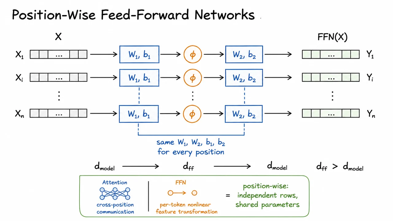
After multi-head attention has gathered information from different positions and different representation subspaces, the Transformer still needs a way to compute new features from the resulting token vectors. Attention is excellent at routing and mixing information across the sequence, but the weighted sums it produces are still largely linear combinations of value vectors. To make each token representation more expressive, every Transformer block follows attention with a position-wise feed-forward network.
The phrase position-wise is important. Suppose the block input is a matrix
where row is the representation of token position , already combining token identity and positional information. After multi-head attention, each row has had the opportunity to receive information from other rows. The feed-forward layer then applies the same nonlinear map to each row independently:
Here are shared across all positions, and is a pointwise nonlinearity such as ReLU or GELU. In modern Transformers, GELU-like activations are common, but the architectural idea is not tied to one particular choice.
A useful mental model is that attention answers the question: Which other positions should this token read from? The feed-forward network answers a different question: Given the information now stored in this token vector, how should we transform its features? These are complementary operations:
This independence means there is no communication between positions inside the FFN itself. If position affects position , that influence must have already been routed through attention or must happen in a later attention layer. The FFN is therefore not a replacement for attention; it is the nonlinear feature processor that acts after attention has assembled a useful local representation at each position.
The standard Transformer FFN has a characteristic expand-and-compress shape:
The first linear map projects each token vector into a wider hidden space of dimension . The activation introduces nonlinearity, allowing the model to form feature interactions that cannot be represented by attention’s weighted averaging alone. The second linear map compresses the representation back to , so the output can be passed cleanly to the next sublayer in the block.
This expansion matters. If the FFN were only a single linear map from to , then it would add limited expressive power, especially when surrounded by other linear projections. The intermediate width gives the model a larger workspace for computing token-wise features: detecting patterns, gating dimensions, composing semantic attributes, or re-encoding information gathered from attention. In many Transformer configurations, is several times larger than , making the FFN a major contributor to both parameter count and computation.
There is a subtle but important symmetry here. Because the same FFN parameters are applied to every row, the operation is shared over sequence length. The model does not learn one feed-forward map for the first token, another for the second token, and so on. Instead, positional differences are represented in the input vectors themselves, while the transformation rule remains the same everywhere. This sharing is one reason Transformers can process variable-length sequences: the FFN does not depend on a fixed sequence length .
Equivalently, we can view the FFN as a tiny multilayer perceptron applied in parallel to all token positions. In matrix form, ignoring broadcasting details for the biases, this is
but this compact expression can hide the crucial fact that row is transformed without directly reading row . The matrix notation is efficient; the row-wise interpretation is the architectural insight.
The visual below condenses this idea into a left-to-right pipeline. Each row vector enters an identical two-layer nonlinear transformation: expansion by , activation by , and compression by . The parallel lanes emphasize that there are no arrows between positions inside the FFN.
The shared-weight annotation is just as important as the lanes themselves. It reminds us that the FFN is independent across rows but not separately parameterized across rows. The same learned map is reused at every position, turning attention’s cross-token communication into richer per-token features before the block moves on to residual connections and normalization.
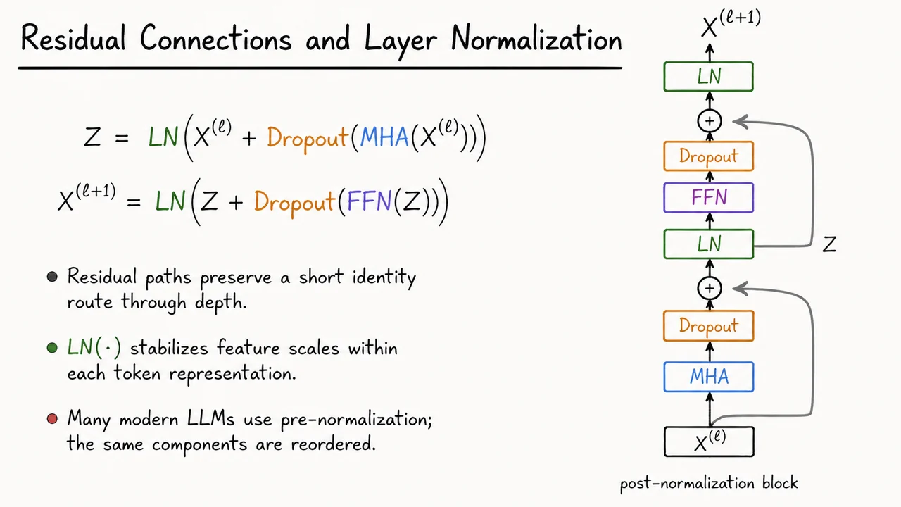
After adding the position-wise feed-forward network, we now have the two computational ingredients that make up a Transformer block: multi-head attention for token-to-token interaction, and an MLP/FFN for per-token nonlinear transformation. But simply stacking these transformations naively is usually unstable. Deep networks need a way to preserve information, keep gradients healthy, and prevent activations from drifting into poorly scaled regimes.
This is where the Transformer block becomes more than “attention followed by an MLP.” Each major sublayer is wrapped with three stabilizing mechanisms:
In the original Transformer formulation, these are arranged in a post-normalization pattern. For an input sequence representation , the attention sublayer produces an intermediate representation
Then the feed-forward sublayer is applied with the same wrapper:
The residual addition is not just a convenience. It gives the block a short identity route through depth. If the attention or feed-forward transformation is initially unhelpful, the model can still pass forward something close to the original representation. This matters because deep Transformers are trained by gradient descent: without residual paths, every layer would have to learn both how to preserve useful information and how to modify it. With residual paths, a sublayer can instead learn a correction or update to the current representation.
A useful way to think about one wrapped sublayer is
Attention contributes a context-dependent update, while the FFN contributes a token-wise nonlinear update. The residual path ensures that these updates are added to an existing representation rather than replacing it entirely. This “incremental refinement” viewpoint is one reason very deep residual architectures are trainable.
Dropout is placed on the sublayer output before the residual addition. During training, this randomly removes parts of the proposed update. The identity path remains intact, so dropout regularizes the transformation without fully corrupting the information stream. In other words, the model is discouraged from relying too heavily on any one attention head, hidden feature, or feed-forward activation, while still preserving a stable baseline signal through the residual branch.
Layer normalization then controls the scale of the resulting token representations. For each token independently, layer normalization computes statistics across the feature dimension and normalizes the vector. Abstractly, for a token vector ,
where and are computed over the features of that token, and are learned scale and shift parameters. This differs from batch normalization: the normalization does not depend on other examples in the batch or other positions in the sequence. That property is especially important for variable-length sequence models and autoregressive decoding.
There is a subtle but important architectural variation here. The equations above describe post-normalization, where normalization happens after the residual addition. Many modern large language models instead use pre-normalization, where the input is normalized before the attention or FFN sublayer, and the residual addition happens afterward. The ingredients are the same, but the order changes:
Pre-normalization often improves optimization stability for very deep Transformers because gradients can flow more directly through the residual stream. Post-normalization was used in the original Transformer and remains conceptually clean, but it can become harder to train as depth increases unless additional care is taken with initialization, learning-rate schedules, or normalization variants.
The visual below should now read as a compact assembly diagram for the post-normalization Transformer block. The main vertical path applies MHA and then FFN, while the curved bypass arrows represent the residual identity routes. Each learned update passes through Dropout, is added back to the incoming representation, and is then stabilized by LN.
The key idea is that the block is not a plain stack of transformations. It is a repeated pattern of propose an update, regularize it, add it to the residual stream, normalize the result. That pattern is what lets attention and feed-forward layers be composed deeply enough to form the backbone of modern Transformer models.
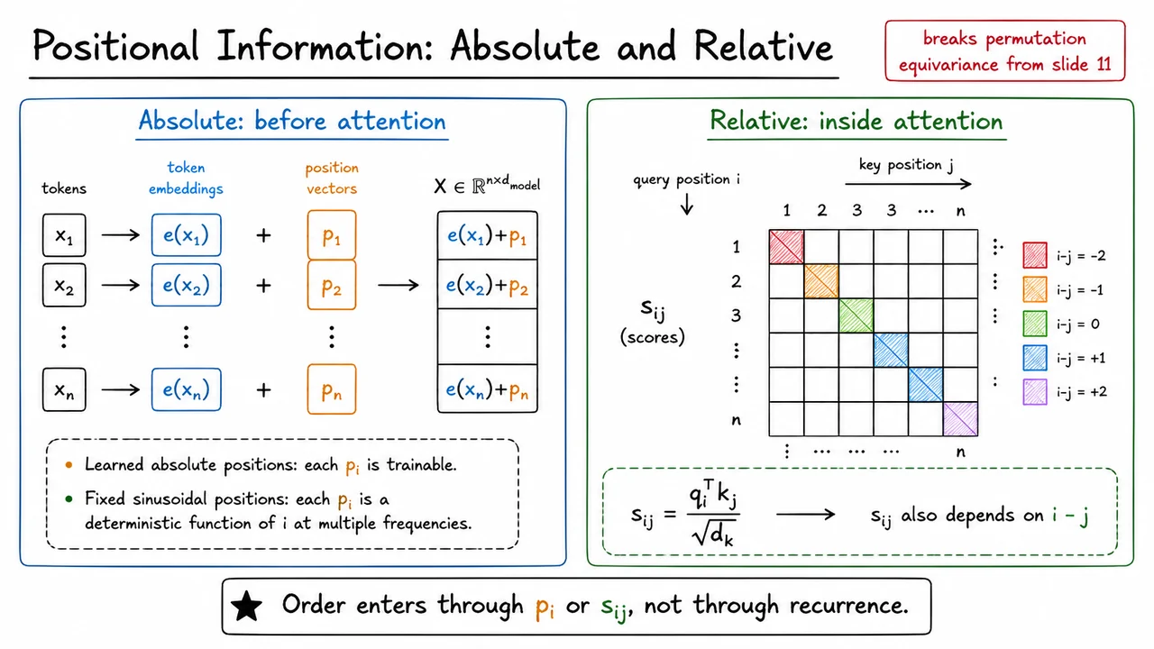
With residual connections and layer normalization in place, a Transformer block has a stable way to transform and refine representations. But there is still a surprisingly fundamental problem: self-attention itself does not know what order the tokens came in.
The reason is that vanilla self-attention is a content-based retrieval mechanism. Each token produces a query, key, and value; attention compares queries to keys and mixes values according to similarity. If we permute the rows of the input matrix , then the queries, keys, values, attention weights, and outputs are permuted in the same way. In other words, self-attention is permutation equivariant: reordering the input sequence merely reorders the output sequence. That is a useful symmetry for sets, but language is not a set. The sentences “dog bites man” and “man bites dog” contain the same words, but their meanings are not interchangeable.
So the Transformer must break this symmetry deliberately. It does not do so by recurrence, where position is implicit in the order of computation, nor by convolution, where locality is built into the kernel geometry. Instead, it injects position information into an otherwise order-agnostic attention mechanism. Broadly, there are two families of solutions:
The original Transformer used absolute positional encodings. If is the token embedding for token , then we add a position vector before the first attention layer:
This changes the meaning of the row representation. A row no longer says only “this is the word bank”; it says something closer to “this is the word bank at position .” Once that information is inside the representation, the attention mechanism can learn position-sensitive behavior through ordinary dot products. For example, a head may learn that a token near the beginning of a sentence behaves differently from the same token near the end, or that certain syntactic patterns depend on approximate position.
There are two common variants of absolute positions. In learned absolute positions, each is a trainable vector, just like a word embedding. This is simple and flexible, but it ties the model to the range of positions seen during training unless special care is taken. In fixed sinusoidal positions, is a deterministic function of , using sine and cosine waves at multiple frequencies. The motivation is that different dimensions encode position at different resolutions, and relative offsets can be expressed through linear relationships among these periodic features. Fixed encodings are not learned from data, but they provide a structured notion of position that can extrapolate more gracefully in some settings.
Absolute positions are intuitive, but they have a subtle limitation: they identify where a token is in the sequence, not directly how far apart two tokens are. Many linguistic and sequential patterns are naturally relative. A word may care about the previous token, the next token, the nearest verb, or another symbol three positions back. For these cases, it is often more natural to inject order into the attention score itself.
In standard scaled dot-product attention, the score from query position to key position is
Relative positional methods modify this idea so that the score also depends on the displacement between the two positions:
This is a different way of breaking permutation symmetry. Instead of saying “token carries position vector ,” the model says “when position attends to position , the interaction depends on their distance and direction.” The sign of matters: attending three tokens to the left is not the same as attending three tokens to the right. In practice, this can be implemented using additive biases, relative key/value embeddings, rotary transformations, or other mechanisms, but the conceptual move is the same: make attention pairwise position-aware.
The distinction matters because each approach gives the model a different inductive bias. Absolute positions are simple and global: every token knows its address. Relative positions are relational: every attention edge knows its offset. Absolute positions can be enough for many tasks, especially when sequence lengths are bounded and consistent. Relative schemes often work better when patterns depend on local displacement, when length extrapolation matters, or when the model benefits from treating “nearby” and “far away” interactions differently regardless of absolute location.
The visual below consolidates these two routes into the same conceptual frame. On the left, order enters before attention: token embeddings are combined with position vectors , producing the matrix . On the right, order enters inside attention: the score grid is no longer determined only by content similarity , but also by diagonal bands corresponding to relative offsets .
The key takeaway is that Transformers do not obtain order “for free.” Self-attention gives them flexible content-based communication, residual paths preserve and refine representations, and layer normalization stabilizes the computation—but positional information is what turns a permutation-equivariant set processor into a sequence model. Order enters either through the representation , or through the attention interaction , rather than through recurrence.
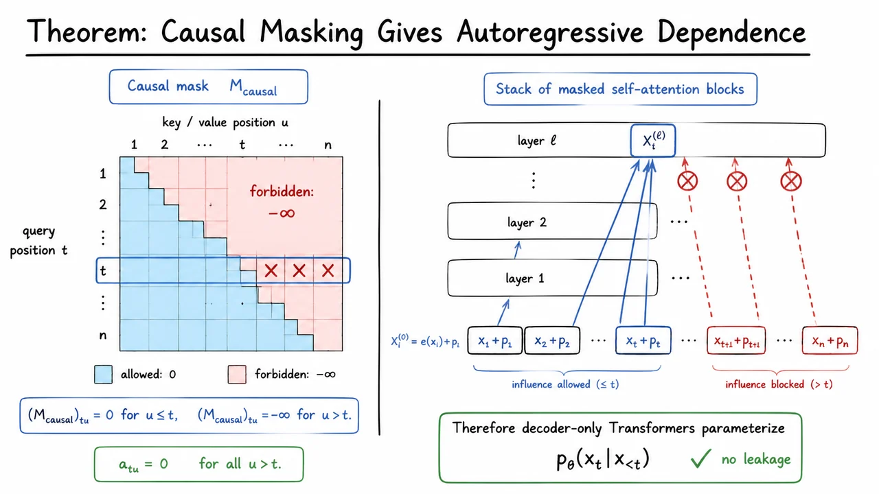
After adding positional information, we have fixed one major ambiguity of self-attention: a token representation can now know where it sits. But in the decoder there is a second, equally important constraint: it must not know what comes next. If a model is trained to predict the next token while its internal representation can already attend to future tokens, the learning problem becomes contaminated by future-token leakage. The model may appear to achieve excellent training loss, but it is solving the wrong conditional distribution.
The autoregressive modeling assumption is that a sequence distribution factors as
So when the model produces the conditional distribution for position , its computation may depend on , but not on depending on the exact indexing convention. Equivalently, if we feed the decoder a prefix ending at position , the representation at that position may depend only on the prefix. In the common teacher-forcing setup, inputs are shifted so that the row at one position is used to predict the next token; the same structural requirement remains: no representation used for prediction may incorporate information from tokens to its right.
Causal masking enforces this directly inside self-attention. Recall that attention weights are computed from logits of the form
followed by a row-wise softmax over key/value positions . In decoder self-attention, the additive mask is
Thus, for query position , keys and values at positions receive logit . After softmax, their probability mass is exactly zero:
This is the key mechanism. The mask does not merely discourage looking ahead; in the mathematical idealization, it removes those edges from the computation graph.
Now consider a full stack of masked Transformer decoder blocks. The input at position is
where is the token embedding and is positional information. The theorem says that for every layer and every position , the row is a function only of
not of any future token with . This is what makes decoder-only Transformers valid autoregressive models: their internal states respect the same left-to-right conditional structure as the probability distribution they are trained to represent.
The proof is a simple but important induction over layers. At layer , the row depends only on and , so it certainly does not depend on future tokens. Assume that at layer , every row depends only on tokens up to position . When computing masked self-attention for row at the next layer, the query at can attend only to rows . By the induction hypothesis, each such row depends only on tokens , and since , all of those are contained in . Therefore the attention output at position depends only on the prefix up to .
The remaining parts of the Transformer block preserve this property. The feed-forward network is applied position-wise, so it cannot mix information across sequence positions. Residual connections add together quantities from the same row. Layer normalization, in the usual Transformer form, normalizes across feature dimensions within a row, not across time positions. Therefore residual-plus-normalization also cannot introduce dependence on future tokens. The induction closes: every layer preserves the causal dependency structure.
There are a few subtle assumptions hiding inside this clean theorem:
In real implementations, is often approximated by a very large negative number. This is usually safe in floating-point arithmetic, but conceptually the theorem relies on the masked attention weights being exactly zero for future positions. Bugs in masking, off-by-one indexing errors, or applying the mask with the wrong tensor shape can produce silent leakage. Such leakage is especially dangerous because training loss may improve while generation quality or evaluation validity becomes compromised.
The practical payoff is that we can train on full sequences in parallel while still modeling left-to-right conditionals. During training, the model sees the entire length- sequence as a tensor, but the causal mask ensures that the representation used for each prediction only has access to the appropriate prefix. This is the core reason Transformer decoders avoid the sequential computation bottleneck of RNNs while still parameterizing distributions like
The visual below compactly summarizes the theorem’s two perspectives. On the left, the causal mask is a lower-triangular attention pattern: positions may attend backward and to themselves, but the strict upper triangle is removed. A highlighted query row makes the statement concrete: all entries with are blocked, which corresponds exactly to .
On the right, the same idea is lifted from one attention matrix to an entire stack of decoder blocks. Information from positions can flow upward into , while arrows from future positions are stopped before reaching it. That is the theorem in computational-graph form: after any number of masked self-attention layers, the row used for autoregressive prediction still depends only on the prefix, giving next-token modeling with no leakage.
The causal masking theorem gives us more than a correctness condition for language modeling. It tells us that attention is a programmable dependency pattern: by changing which positions are allowed to communicate, we change the computational graph of the model without changing the basic attention mechanism itself.
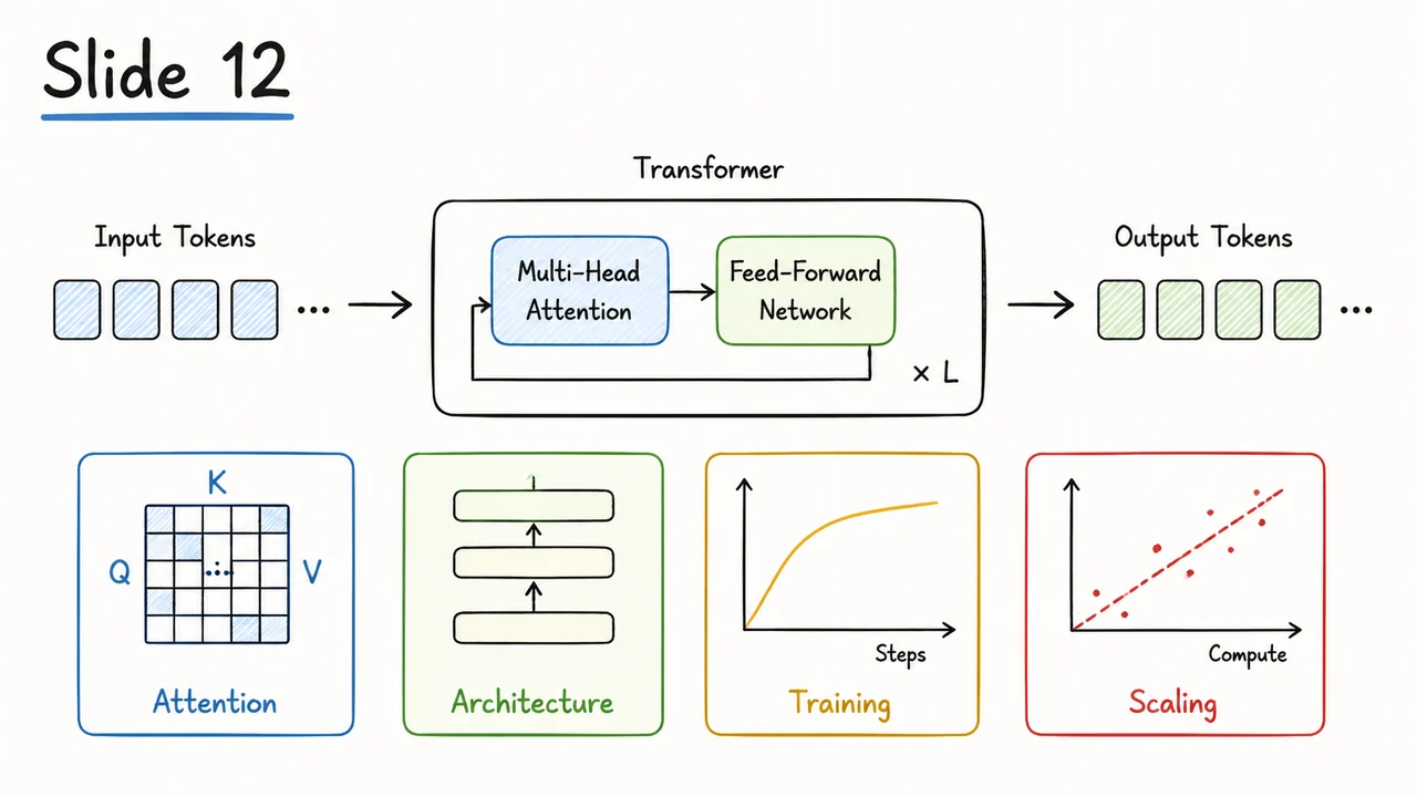
That is the key architectural leap. A Transformer is not “an attention layer” repeated many times in the abstract. It is a stack of modules where each module answers three separate questions:
The previous result focused on the first question for autoregressive models. If token is only allowed to attend to positions , then its representation cannot depend on future tokens. That makes next-token prediction valid: the model cannot “cheat” by reading the answer from the right-hand side of the sequence.
But causal masking is only one possible attention topology. The same attention operation can support very different modeling regimes depending on the allowed communication pattern:
A useful way to think about this is that attention defines a soft message-passing graph over token representations. The mask determines which edges exist; the attention scores determine how strongly each available edge is used. The model does not merely copy from neighboring positions. It learns, at every layer and every head, which previous or external states are relevant to the current computation.
This separation matters because many Transformer properties come from structural constraints, not from learned parameters alone. If we remove the causal mask from a language-model decoder during training, the model may achieve an artificially low loss by using future tokens. If we impose a causal mask inside an encoder, we unnecessarily prevent tokens from using right context. If we omit positional information, self-attention remains largely insensitive to token order except through whatever asymmetries are introduced elsewhere. The architecture works because these design choices are aligned with the task.
There is also a computational reason to keep these pieces modular. During training, even causal self-attention can be evaluated in parallel across all positions because the mask is known in advance. The model computes all token representations simultaneously while enforcing the same dependency pattern that will hold during generation. During decoding, however, generation is sequential: after predicting one token, the model appends it to the prefix and runs the next step. This is why training and inference have different bottlenecks even though they use the same learned layers.
The next architectural step is therefore to assemble these attention patterns into reusable blocks. Each block takes a sequence of hidden states, routes information through an attention sublayer, applies a token-wise feed-forward transformation, and preserves trainability through residual and normalization structure. The distinction between encoder, decoder, and encoder-decoder models is mostly a distinction in which attention sublayers are present and what they are allowed to see.
The visual below serves as a compact transition from the theorem to the architecture. Instead of treating masking as a small implementation detail, it places masking and attention access patterns at the center of the design. Once that picture is clear, encoder self-attention, decoder causal self-attention, and cross-attention become variations of the same underlying operation rather than separate mechanisms.
It is worth carrying this mental model forward: attention computes content-based retrieval; masks define legal information flow; Transformer blocks package that retrieval into stable, trainable layers. With that in place, we can now build the encoder, decoder, and encoder-decoder Transformer architectures systematically.
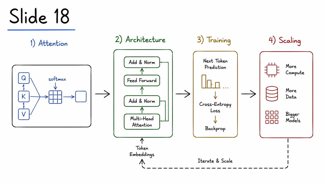
A useful way to organize the Transformer design space is to stop thinking in terms of “different architectures” and instead ask two more primitive questions: which tokens are allowed to attend to which other tokens, and where do the queries, keys, and values come from? Once causal masking is understood, the distinction between encoder-only, decoder-only, and encoder–decoder Transformers becomes much less mysterious. They are mostly the same attention operation, wired with different masks and different source streams.
Recall the core attention computation:
The matrix scores how much each query position wants to retrieve information from each key position. The mask then changes which retrievals are legal. Typically, allowed entries receive , while forbidden entries receive a very negative number, effectively making their softmax probability zero. So the mask is not a minor implementation detail; it defines the information flow graph of the model.
In an encoder-only Transformer, all positions in the input sequence can usually attend to all other non-padding positions. There is no causal restriction because the goal is not to generate the sequence left-to-right. Instead, the model builds a contextual representation , where each token representation may depend on tokens both to its left and to its right. This is appropriate for tasks like classification, retrieval, tagging, and masked-token prediction, where the entire input is available at once.
The subtle assumption here is that bidirectional context is legal. If the downstream task requires predicting the future from the past, an encoder-only model would leak information unless we carefully modify the objective or mask. But when the whole input is genuinely observed, full self-attention is a strength: every token can be interpreted in light of the complete sequence.
In a decoder-only Transformer, the same sequence is treated as a language-modeling sequence. Position is trained to predict the next or current token using only earlier tokens. The model therefore uses causal self-attention, meaning token may attend to positions , but not to positions . This gives the familiar autoregressive factorization:
This architecture is natural for open-ended generation because the model’s training-time information pattern matches its test-time use: when generating token , the future tokens do not yet exist. A failure mode appears when this alignment is broken. If a decoder accidentally receives unmasked future tokens during training, it can learn a shortcut that disappears at inference time. Causal masking is therefore what makes parallel training compatible with left-to-right generation.
An encoder–decoder Transformer separates the problem into two streams. The encoder first reads the source sequence and produces contextual representations . The decoder then generates a target sequence autoregressively. Within the decoder, causal self-attention ensures that position can only depend on . But after that, the decoder also performs cross-attention over the encoder output. This gives the conditional prediction form
Cross-attention is not a new mathematical primitive. It is the same content-based retrieval operation, but with a different source for . The decoder state supplies the queries : “given what I have generated so far, what source information do I need?” The encoder output supplies the keys and values : “here are the source-side memories available for retrieval.” In compact form,
This distinction matters because it separates two kinds of dependency. Decoder self-attention models dependencies among generated target tokens, while cross-attention conditions those target tokens on the input. For translation, summarization, speech recognition, and other sequence-to-sequence tasks, this is exactly what we want: the output should be fluent in its own sequence while remaining grounded in the source.
The three families can therefore be compared by a small set of choices:
The visual below condenses this taxonomy into a table: the rows are not fundamentally different attention formulas, but different choices about masks and streams. The important thing to notice is that “self-attention” means come from the same sequence, whereas “cross-attention” means the decoder provides and the encoder provides .
The equation at the bottom reinforces the main point: all three cases still use scaled dot-product attention. What changes is the mask and the provenance of the matrices. Once that is clear, the transition to training objectives becomes straightforward: each architecture defines which conditional distribution it is allowed to model, and the next step is to train those conditionals by maximum likelihood.
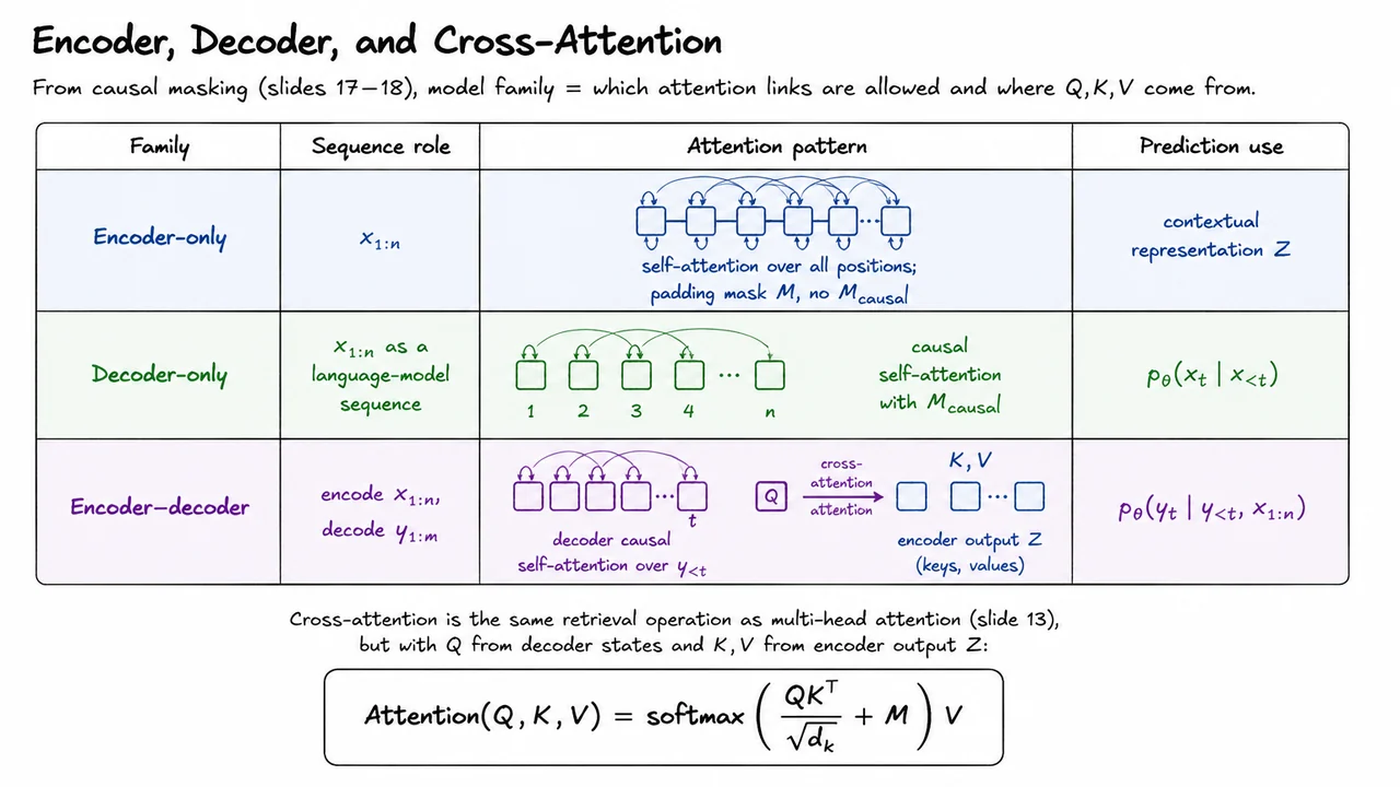
Having separated the Transformer into encoder, decoder, and cross-attention components, the next question is: what exactly do we optimize during training? The architecture gives us a conditional distribution over tokens, but training turns that distribution into a supervised learning problem repeated across every position in a sequence.
For an encoder-decoder Transformer, the target sequence is generated autoregressively conditioned on the source sequence . That means we model the joint conditional probability by the chain rule:
This factorization is not an approximation by itself; it is just the probability chain rule. The modeling assumption enters through the Transformer parameterization of each conditional distribution . At position , the decoder is supposed to use the source representation from the encoder and the already generated target prefix , but not the future target tokens .
This is where teacher forcing enters. During training, we do not ask the model to generate its own prefix token by token and then learn from the resulting rollout. Instead, for every position , we feed the decoder the ground-truth prefix. The model sees the correct previous tokens and is trained to predict the next one:
The subtle but crucial detail is that the model may receive the full target sequence as a tensor during the forward pass, but the causal mask ensures that position can only attend to positions . Without this mask, the decoder could leak information from or , making the training loss artificially low and destroying the intended autoregressive semantics.
The maximum-likelihood objective asks us to maximize the probability of the observed target sequences under this factorization. Equivalently, we minimize the negative log-likelihood:
In practice, this is exactly the usual cross-entropy loss over the vocabulary at every decoder position. The decoder outputs a vector of logits at each position; after a softmax, the probability assigned to the correct next token is selected, logged, negated, and summed. Because the correct prefix is supplied everywhere, every target position contributes a supervised training signal in one forward pass.
This is one of the key computational advantages of Transformer training. Although the probability model is autoregressive, the training computation is parallel over positions. We do not have to run the decoder once for , then again for , and so on. Instead, the causal mask gives each position the right information boundary, allowing all next-token predictions to be trained simultaneously:
For decoder-only language modeling, the same idea applies after removing the source sequence. A language model learns to predict each token from its left context:
This is the objective behind standard autoregressive pretraining. The “input” and “target” are shifted versions of the same sequence: the model consumes previous tokens and predicts the next token. Again, the causal mask is what makes it legitimate to process the entire sequence at once while preserving the left-to-right conditional structure.
There is an important distinction between training and decoding here. During training, teacher forcing conditions on the true prefix, so all positions are supervised in parallel. During inference, the true prefix is unavailable; the model must condition on tokens it has already generated. This creates exposure to its own mistakes, and it also makes decoding sequential in the output length. Thus, Transformers train highly parallelly but still generate autoregressively unless we change the modeling assumptions.
The visual summary below compresses this objective into three pieces: the autoregressive factorization, the encoder-decoder negative log-likelihood, and the decoder-only language modeling loss. The highlighted prefixes and are the conditioning contexts supplied under teacher forcing, while the causal mask marks the boundary that prevents a position from seeing future tokens.
The small token timeline reinforces the operational meaning of the equations: every position is trained as a next-token prediction problem, but the red barrier imposed by the causal mask keeps each prediction honest. This is the central training recipe for sequence Transformers: sum cross-entropy over examples and positions, with ground-truth prefixes and no future-token leakage.
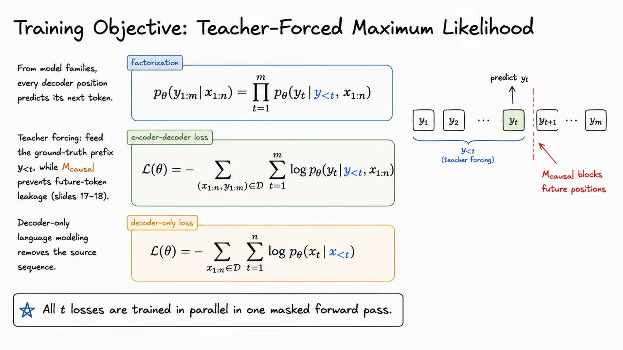
Having defined the teacher-forced likelihood objective, we now need to be precise about what the model actually computes before that objective is evaluated. For an encoder-only Transformer, the forward pass is conceptually simple: convert a sequence of tokens into a sequence of contextual vectors, repeatedly allowing each position to retrieve information from other positions and then transform its own representation through a shared nonlinear map.
The input is a token sequence . Since attention by itself is permutation-equivariant, the encoder must be given some representation of order. The usual first step is therefore to add a learned or fixed positional vector to each token embedding :
Here each row of is the representation of one token position. The matrix shape matters: the encoder preserves the sequence length throughout the stack, while updating the -dimensional representation at each position. This is one reason encoders are reusable: their output is still a sequence, not a single collapsed vector.
Each encoder layer then applies two sublayers. The first is multi-head self-attention, where every position forms queries, keys, and values from the current sequence representation. Within each head, attention weights are computed as
The mask is especially important in batched training. For a standard bidirectional encoder, we usually do not use a causal mask, because each token is allowed to attend to tokens on both its left and right. But if examples have been padded to a common length, padded positions must not participate as real content. This is handled by adding a padding mask before the row-wise softmax, typically using large negative values so that attention probability on padded keys becomes essentially zero.
After attention, the encoder does not simply replace with . Instead it uses a residual connection, dropout, and layer normalization:
The residual path is not just an implementation detail. It gives the layer an easy way to preserve existing information, improves gradient flow through deep stacks, and lets attention learn corrections rather than recomputing the entire representation from scratch. Layer normalization then stabilizes the scale of activations at each position, which becomes increasingly important as , the number of layers, grows.
The second sublayer is the position-wise feed-forward network:
“Position-wise” means the same multilayer perceptron is applied independently to each row of . Attention is the mechanism that mixes information across positions; the feed-forward network is the mechanism that applies a richer nonlinear transformation within each position. This separation is one of the clean design principles of the Transformer block:
A subtle but useful way to view the encoder is as a repeated refinement process. At layer , a token’s representation may mostly encode lexical identity and position. After several layers, that same row can encode syntactic role, semantic relationships, discourse context, or task-relevant features—while still occupying the same sequence slot. The algorithm returns the final matrix , whose rows are contextual embeddings. Depending on the task, this matrix might feed a classifier, a retrieval head, a token-level predictor, or the cross-attention module of a decoder.
The main failure mode to watch for is confusing the encoder mask with the decoder mask. In an encoder, the mask is usually about padding, not causality. If we accidentally apply a causal mask inside a bidirectional encoder, we restrict the model unnecessarily and change its equivariance properties. Conversely, if we forget the padding mask, real tokens may attend to padding embeddings, allowing meaningless positions to contaminate the contextual representations.
The visual below packages this forward pass as an algorithm: initialize token-plus-position representations, loop through identical encoder blocks, apply masked multi-head self-attention with residual normalization, then apply the shared position-wise feed-forward update with another residual normalization. The right-hand stack view is a useful mental model: the sequence enters at the bottom, is lifted into , passes through repeated encoder layers, and exits as a contextual sequence representation.
Read the pseudocode not as a low-level implementation prescription, but as the mathematical skeleton of the encoder. Actual implementations may choose pre-norm instead of post-norm, fuse projections for efficiency, or batch many sequences together, but the invariant structure remains the same: self-attention mixes tokens, the FFN transforms positions, and the stack preserves sequence shape while enriching representation quality.
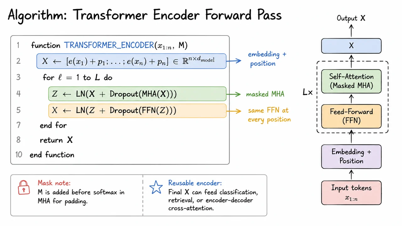
Once we know how a Transformer produces hidden states through a forward pass, training becomes almost surprisingly ordinary. The architectural details may differ—encoder-only classification, decoder-only language modeling, encoder-decoder translation—but the core optimization loop is the familiar one: sample a minibatch, run the model, compare predicted token distributions to the correct next or target tokens, and update parameters by gradient descent.
For sequence generation, the key supervision signal is cross-entropy over vocabulary logits. At each target position , the final Transformer representation is projected into vocabulary space:
Here is not yet a probability distribution; it is a vector of unnormalized scores, one per vocabulary item. Applying softmax converts those scores into a categorical distribution over the next token, and the loss penalizes the model when it assigns low probability to the correct token :
The phrase non-padding is more important than it may look. In minibatch training, sequences are usually padded to a common length so they can be represented as a dense tensor. Padding tokens are not real targets; if we included them in the loss, the model would waste capacity learning to predict artificial batch-formatting artifacts. Thus padding positions are masked both in attention, where they should not be read as content, and in the loss, where they should not contribute gradients.
For decoder training, the central trick is teacher forcing. Instead of generating tokens one at a time during training, we feed the model the ground-truth prefix and ask it to predict each next token in parallel. For a target sequence , the decoder receives shifted inputs such as and is trained to predict . Because causal masks prevent position from seeing future target tokens, this parallel computation is still faithful to the autoregressive factorization:
This is one of the major computational advantages of Transformers over recurrent sequence models. At inference time, autoregressive decoding must still proceed token by token, because each generated token becomes part of the next input. But during training, the entire target sequence can be processed simultaneously under a causal mask. The model is therefore trained on all positions in a minibatch with a single parallel forward pass.
The precise interpretation of the target token depends on the model family:
Once the loss is computed, training updates all parameters by differentiating through the entire computation graph: embeddings, attention projections, feed-forward layers, normalization parameters, and the vocabulary projection. In its simplest gradient-descent form, the update is
where is the learning rate. In practical Transformer training, this step is usually performed by Adam or AdamW rather than plain gradient descent, often with learning-rate warmup, weight decay, gradient clipping, mixed precision, and distributed data parallelism. But those engineering choices refine the same mathematical loop: minimize token-level negative log-likelihood over minibatches.
A useful way to view the whole algorithm is as a tension between parallelism during training and causality in the model definition. Teacher forcing exposes every target position at once, but causal masking ensures that the representation at position cannot depend on target tokens after . Padding masks remove fake tokens introduced by batching. Cross-entropy then turns each valid target position into a supervised classification problem over the vocabulary.
The visual summary condenses this into the training loop you would actually implement: initialize parameters, sample a minibatch, run the relevant Transformer forward pass, compute logits, accumulate masked cross-entropy over non-padding targets, and update . The highlighted lines emphasize the three mathematical operations that matter most: vocabulary projection, likelihood loss, and gradient update.
The callouts also mark the two assumptions that are easy to forget when reading pseudocode too quickly. First, the forward pass depends on which Transformer family is being trained—encoder, decoder-only, or encoder-decoder. Second, the loss is teacher-forced and padding-aware: all valid target positions contribute in parallel, while masked or padded positions do not.
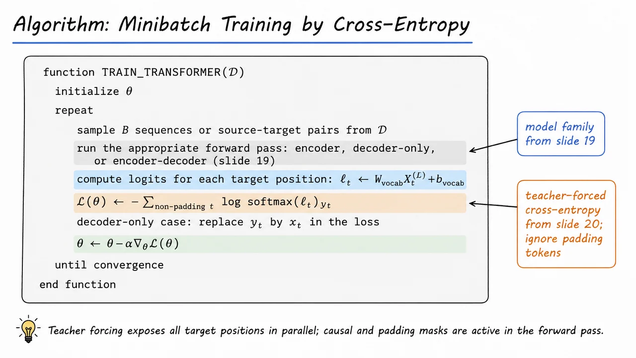
After training with cross-entropy, it is tempting to think of the Transformer decoder as producing an entire output sequence in one forward pass. During teacher forcing, that is almost true computationally: we feed the ground-truth prefix at every position, apply the causal mask, and evaluate all next-token losses in parallel. But at test time the ground-truth prefix is gone. The model must condition on its own previous predictions, so generation becomes an explicitly sequential process.
The model defines a conditional distribution for the next token,
where is the source/input sequence and is the prefix already generated. The hats matter: these are not gold tokens anymore. They are decisions made by the model at earlier decoding steps. Once the model chooses , that token becomes part of the context used to choose , and so on.
In greedy decoding, the decision rule is the simplest possible one: at each step, choose the most likely next token under the current model distribution,
This looks locally optimal, but it is not globally optimal in general. A token that is best at time may lead to a poor continuation later, while a slightly less likely token might open up a much better full sequence. Greedy decoding is therefore fast and deterministic, but it can be shortsighted.
The causal mask remains essential during decoding. Even though we generate left-to-right, each forward pass still computes attention over the current prefix positions. The mask enforces the autoregressive factorization: token may attend to , but not to future tokens that have not yet been produced. Conceptually, decoding constructs the sequence according to
until a maximum length is reached or a special end-of-sequence token is emitted.
A useful way to write greedy decoding is:
function GREEDY_DECODE(x_{1:n}, T)
    encode x_{1:n} if using encoder-decoder
    initialize \hat{y}_{<1} as the required start context

    for t = 1 to T do
        compute p_\theta(y_t | \hat{y}_{<t}, x_{1:n}) with the causal mask
        \hat{y}_t <- argmax_{y_t in V} p_\theta(y_t | \hat{y}_{<t}, x_{1:n})
        stop if an end token is produced
    end for

    return \hat{y}_{1:t}
end function
The key train-test contrast is that training parallelizes over positions, while decoding does not. During training, the model already has the full target sequence shifted right, so it can compute all conditional distributions in one masked pass. During decoding, however, must be chosen before can even be conditioned on. This dependency chain is fundamental to autoregressive generation.
Beam search relaxes greedy decoding by retaining multiple candidate prefixes instead of only one. At time , it keeps a beam containing the top prefixes, usually ranked by cumulative log-probability:
When , beam search reduces to greedy decoding. Larger beams explore more alternatives, often improving sequence quality, but they increase computation and memory. Beam search is still an approximation: it does not enumerate the exponentially large space of possible sequences, and it may favor short outputs unless length normalization or other scoring adjustments are used.
This decoding process also exposes a subtle failure mode: error accumulation. If the model makes an early mistake, all later predictions condition on that mistake. This differs from teacher-forced training, where the model is usually conditioned on correct prefixes. The mismatch is one reason decoding behavior can be worse than validation cross-entropy alone might suggest.
The visual below condenses the algorithmic structure: initialize a prefix, repeatedly compute the next-token distribution under the causal mask, select a token, append it, and stop on an end token or length limit. The highlighted assignment line is the decisive greedy step—the place where a full probability distribution collapses into one chosen symbol.
It also emphasizes the broader contrast: beam search changes only the number of retained prefixes, not the left-to-right nature of decoding. Whether we keep one prefix or prefixes, generation proceeds token by token because each new prediction becomes part of the next conditioning context.
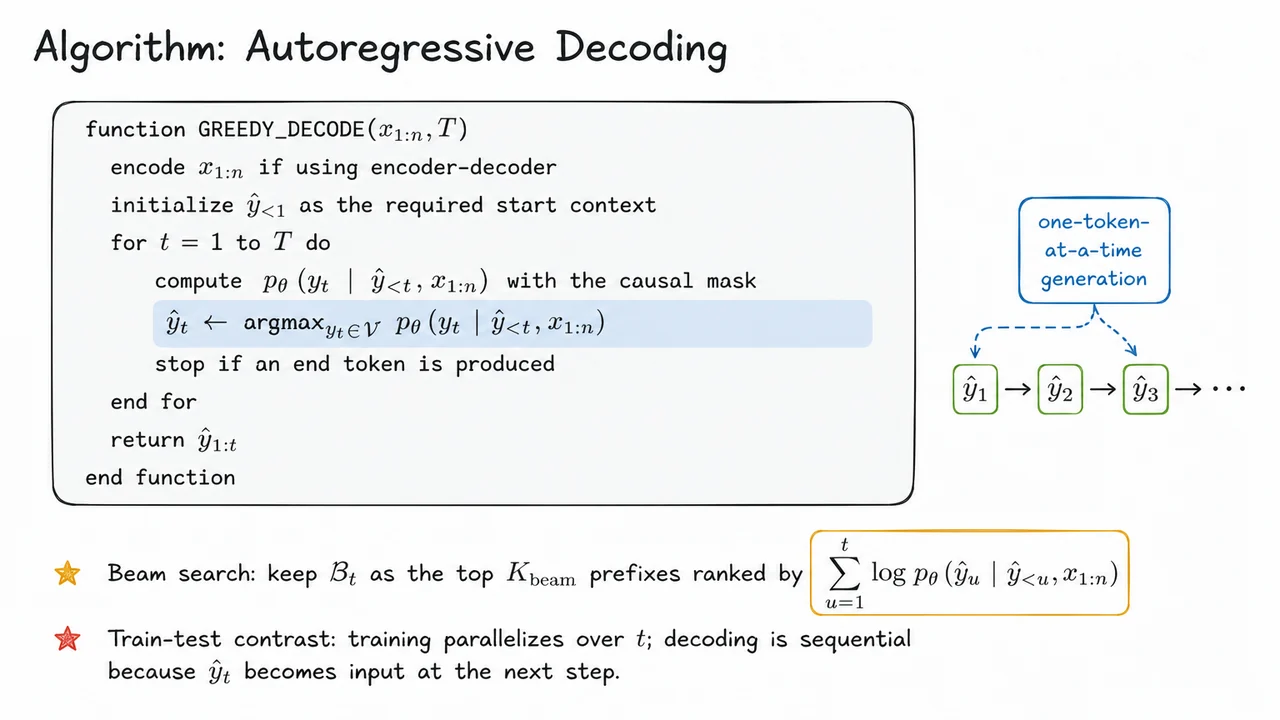
After seeing autoregressive decoding, it is tempting to think of Transformer cost mainly in terms of generation: one token at a time, with a growing key-value cache. But the deeper architectural trade-off is already present inside each layer. A Transformer layer gives every position a direct communication channel to every other position. That is the source of its remarkable parallelism and short dependency paths—but it is also exactly where the quadratic cost enters.
Recall the core operation:
For a sequence of length , the query and key matrices contain one vector per position, so the score matrix satisfies
This matrix is the all-pairs comparison table: position scores position for every pair . In self-attention, the model is not restricted to neighboring tokens or to information carried through a recurrent hidden state. It can ask, in one layer, “which positions in the entire sequence are relevant to this position?”
That global access gives self-attention a constant path length between positions. If token needs information from token , then one attention layer can create a direct edge from to . In graph terms, the self-attention layer behaves like a dense directed graph over sequence positions. The number of computational layers required for information to travel from one token to another is therefore
This is a major contrast with recurrence. In a left-to-right recurrent model, information from an early token must be repeatedly compressed and passed through hidden states before reaching a later token. Even if each recurrent update is powerful, the dependency path between distant positions grows with sequence length:
That long path creates two related problems. First, optimization becomes harder because gradients and information must survive many transformations. Second, training is less parallel across time, since hidden state depends on . Recurrence has attractive linear sequence scaling, but it pays for that with sequential computation and long communication paths.
Convolution sits somewhere in between. A local convolution can process all positions in parallel, which is good for hardware utilization, but each layer only mixes information within a fixed neighborhood. To connect distant tokens, we must stack many layers, use dilation, increase kernel width, or combine these strategies. Thus the effective path length grows with the number of layers needed to cover the distance. Locality is computationally efficient, but global communication is not immediate.
The Transformer chooses the opposite bargain. Full self-attention spends compute and memory to make global communication cheap in depth. Computing the attention scores and applying them to values gives the familiar per-layer scaling
The term comes from storing or materializing the attention matrix , whose entries correspond to pairwise token interactions. The factor appears because those interactions are used to combine vector-valued representations. Exact constants depend on the number of heads, projections, implementation details, and whether intermediate attention matrices are materialized, but the core asymptotic point remains: dense attention scales quadratically in sequence length.
By comparison, a recurrent layer is often summarized as
because each of the steps applies a transformation to a -dimensional state. Local convolution has similar linear dependence on per layer, assuming fixed kernel size, but may require many stacked layers for long-range interaction. So the relevant comparison is not merely “which is cheaper?” but rather:
This trade-off is one of the central reasons Transformers became so effective. They are not efficient because they avoid expensive operations; they are effective because they spend computation in a way that modern accelerators can exploit. A dense attention matrix is costly, but it is also highly parallelizable. During training, all token representations in a layer can be computed simultaneously, unlike recurrent models that must advance through time.
The visual below condenses this argument into a comparison table. The highlighted self-attention row emphasizes both sides of the bargain: the orange terms mark the quadratic cost, while the green path length marks the architectural benefit. The small equation callout ties the cost directly to , reminding us that the all-pairs score matrix is not an implementation accident—it is the defining mechanism of full attention.
The accompanying icons reinforce the same intuition geometrically. Self-attention resembles a fully connected graph over positions; recurrence resembles a chain; local convolution resembles stacked short-range windows. The key takeaway is therefore compact but important: Transformers buy parallel, global communication by paying quadratic scaling in sequence length.
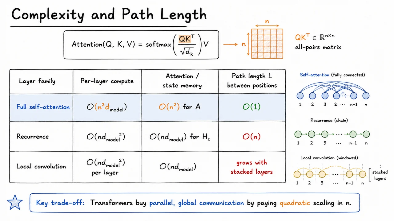
The previous discussion gave us a clean theoretical prediction: if every token can communicate with every other token in one self-attention layer, then the maximum information path length between positions becomes constant,
instead of growing linearly as in recurrence,
or logarithmically under stacked convolutions with expanding receptive fields,
That argument is elegant, but by itself it is not enough. A shorter path length is only useful if the model can exploit it in a real learning problem, under realistic optimization and hardware constraints. The original Transformer paper mattered because it turned this architectural claim into an empirical result: on large-scale machine translation, replacing recurrence and convolution with attention was not merely conceptually simpler—it was faster to train and more accurate.
The canonical benchmark was WMT 2014 machine translation, especially English-to-German and English-to-French. These tasks were a natural testbed for sequence-to-sequence models because they require both local phrase modeling and long-range dependency handling: agreement, word reordering, dropped pronouns, clause structure, and context-dependent lexical choices. The Transformer was evaluated as an encoder-decoder model: the encoder builds contextual representations of the source sentence, the decoder generates the target sentence autoregressively, and cross-attention lets each target-side position retrieve relevant source-side information.
Training used the now-standard maximum-likelihood setup with teacher forcing. Given a source sentence and a target sequence , the model is trained to maximize
where the decoder receives the true previous target tokens during training. This is important because the Transformer’s reported advantage was not based on an exotic objective or a different task formulation. It was tested in the same basic supervised translation regime as the recurrent and convolutional systems it replaced.
The main reported quality metric was BLEU, a corpus-level measure based on modified -gram precision with a brevity penalty. BLEU is imperfect: it rewards surface overlap with reference translations and can miss semantic equivalence, discourse quality, or stylistic appropriateness. But as a historical comparison point for WMT machine translation systems, it was the standard scoreboard. So when Transformer-base reached
on WMT14 English-German, and Transformer-big reached
those numbers were meaningful because they exceeded strong recurrent and convolutional baselines on the same benchmark family.
The efficiency result was just as important as the accuracy result. The Transformer-base model achieved its English-German score with a reported training cost of about FLOPs, substantially below many competitive recurrent encoder-decoder systems with attention. Transformer-big used more compute—about FLOPs—but still remained competitive with or better than much more sequential alternatives, and also achieved
on WMT14 English-French.
The subtle point is that this was not simply “a bigger model wins.” In fact, Transformer-base was not the largest or most expensive system in the comparison. Its advantage came from changing the computational geometry of the sequence model. Recurrence has a strong inductive bias for ordered processing, but it also imposes a hard sequential bottleneck: hidden state depends on , which depends on , and so on. This makes both optimization and hardware utilization harder for long sequences. Convolutions improve parallelism, but distant positions still require multiple layers to interact unless the convolutional kernel is very wide or dilated.
Self-attention makes a different trade-off. Each layer pays a quadratic pairwise interaction cost in sequence length, but in exchange it allows content-dependent global communication immediately. A source token near the beginning of a sentence can influence a token near the end through a single attention operation, not through a chain of recurrent updates or a tower of convolutional neighborhoods. That constant path length is not just a theoretical convenience; it changes how gradients, alignments, and contextual evidence move through the network.
There are still caveats. The original translation setting used sequence lengths where quadratic attention was affordable, and the comparison depends on implementation details, hardware, batching, and the exact baselines chosen. BLEU also does not fully capture translation quality. But the empirical lesson survived these caveats: the Transformer converted a structural advantage—parallel global communication—into a practical training advantage. It improved quality while reducing sequential dependence, which is precisely what the path-length analysis suggested should happen.
The visual below condenses this empirical anchor into a compact comparison. The recurrent and convolutional rows represent the pre-Transformer alternatives: respectively stronger sequential dependence with , and improved but still multi-hop communication with . The Transformer rows highlight the key outcome: higher BLEU scores paired with , showing that constant-path self-attention was not just an architectural novelty but a measurable advantage on a demanding benchmark.
Read the table less as a leaderboard and more as evidence for the trade-off we have been building toward. The important pattern is the alignment between shorter communication paths, greater parallelism, and better translation accuracy per reported training cost. This is why the original machine translation result became the empirical anchor for the Transformer architecture.
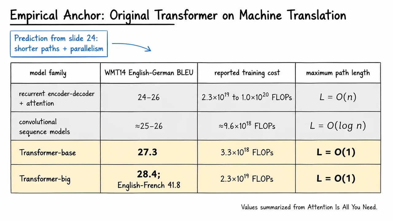
After seeing that the original Transformer worked surprisingly well in machine translation, it is worth slowing down and asking what one of its smallest moving parts is actually doing. The full model is large, multi-layered, and multi-headed, but a single attention head has a very concrete interpretation: it performs a content-based lookup. Given a token position, it asks, “Which other positions contain information useful for updating this representation?” Then it returns a weighted mixture of those positions’ value vectors.
Consider the toy sentence:
“The animal did not cross because it was tired”
Focus on position , the token “it”. In a language understanding setting, a useful head might learn that “it” refers back to “animal”. Importantly, the model is not explicitly given a symbolic coreference rule. Instead, the head computes this relationship through learned vector projections. The hidden state at each position is projected into a query, key, and value:
For the query position , the head scores every candidate position using a scaled dot product:
The dot product is a compatibility score: it is large when the query and key point in similar directions in the learned representation space. The division by is not cosmetic. If the components of queries and keys have roughly unit variance, then an unscaled dot product grows in variance with . Large raw scores can push the softmax into saturation, producing extremely peaked gradients early in training. Scaling keeps the logits in a numerically and statistically healthier range.
Suppose this attention head has learned a roughly coreference-like pattern. For the query token “it”, the score against “animal” might be high, while scores against nearby but less relevant words are lower:
These scores are not yet attention weights. They are unnormalized retrieval logits. The head converts them into a probability distribution over positions using a row-wise softmax:
After normalization, the largest score receives most of the mass. In this illustrative example, the token “animal” might receive weight , while “tired” and “cross” receive much smaller weights, say and . The output of the head at position 7 is then the weighted sum of value vectors:
This is the key operational idea: the representation of “it” is updated by directly mixing in information from “animal”. Unlike an RNN, this path does not require information to be carried step-by-step through the intervening tokens. Unlike a fixed-width convolution, it does not require many stacked layers to connect distant positions. A single attention head can create a direct, data-dependent communication channel between any two positions in the sequence.
There are two subtle points worth keeping in mind. First, the attention weights are content-dependent, not fixed by distance or position alone. A different sentence containing the same word “it” could produce a very different attention pattern. Second, attention weights are not always a faithful human explanation of what the model “believes.” One head may look interpretable, another may spread mass broadly, and another may implement a feature routing pattern that has no simple linguistic label. The computation is still meaningful, but the meaning lives in the learned representation space, not necessarily in our preferred grammatical categories.
The visual below compresses this worked example into the mechanics of one head. The query token “it” sends compatibility scores to all keys, the softmax turns those scores into retrieval weights, and the resulting output vector is dominated by the value at “animal”. The thick arrow represents the high-weight content path; the thinner arrows remind us that attention is usually a mixture, not a hard pointer.
The accompanying bar chart is a useful sanity check: attention for position 7 is a distribution over source positions. If one bar dominates, the head behaves almost like a soft lookup. If the bars are flatter, the head is aggregating broader context. In either case, the computation is the same: score keys against a query, normalize the scores, and return a weighted mixture of values.
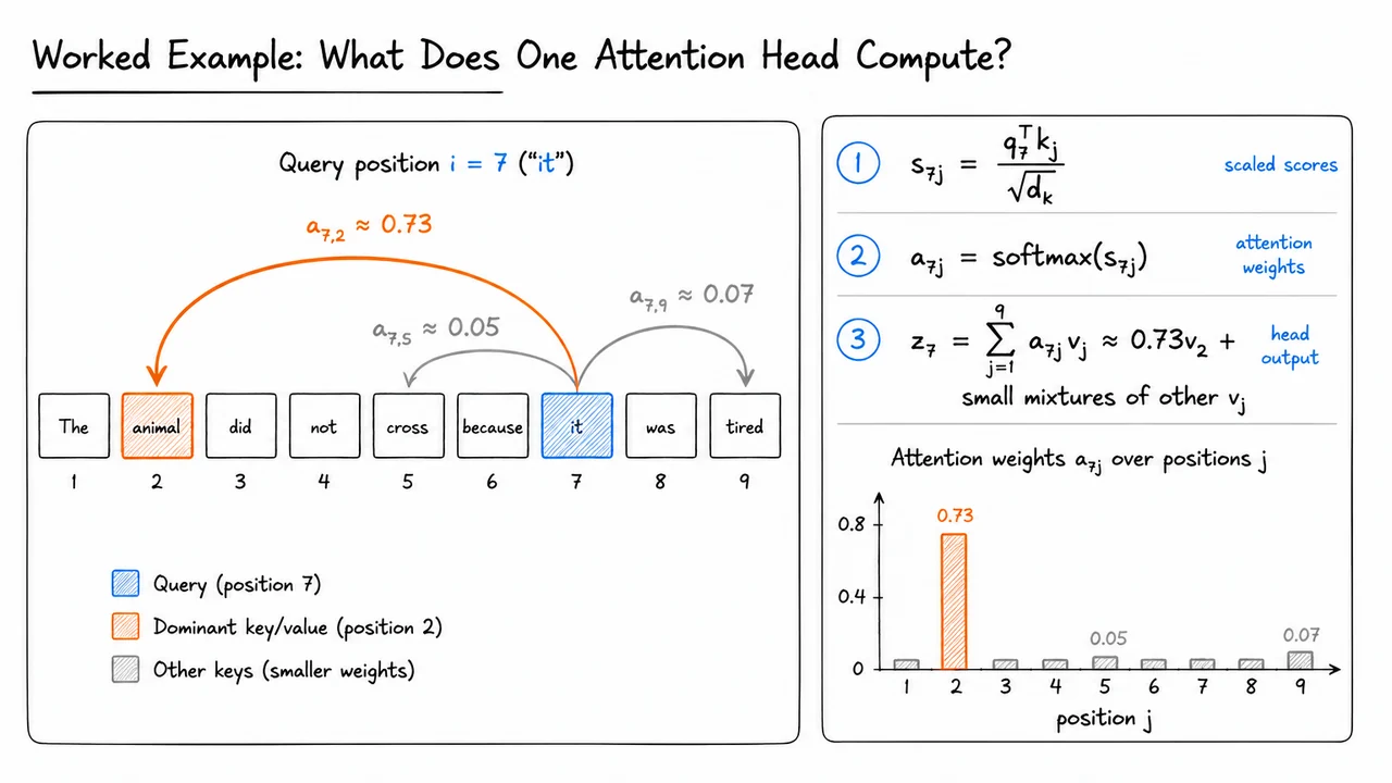
After seeing a concrete attention head in action, it is tempting to think of attention as a nearly ideal communication primitive: every token can look directly at every other token, choose what matters, and aggregate the relevant information in one differentiable step. That intuition is mostly right—and it is exactly why Transformers became so dominant. But the same mechanism that gives self-attention its strength also creates several recurring limitations. The model has global content-based access, not free reasoning, not unlimited memory, and not a guarantee of faithful explanations.
The most basic trade-off is computational. In full self-attention, each of the tokens forms a query and compares it against all keys. This produces an attention score matrix. Even before thinking about values or feed-forward layers, the model has committed to representing all pairwise token-token interactions. Thus attention memory scales as
and the main attention computation scales roughly as
This quadratic dependence is not a small implementation detail; it is a structural property of dense attention. Doubling the sequence length roughly quadruples the number of pairwise scores. For short and medium contexts, this cost is often worth paying because global communication is extremely expressive. For very long contexts, however, the attention matrix becomes a bottleneck in memory, compute, latency, and training batch size. Many efficient-attention variants can be understood as different compromises: sparsify the pairs, compress the memory, chunk the sequence, use recurrence-like state, or approximate the attention kernel. Each saves something, but usually gives up exact dense global access.
A second failure mode is subtler: masking enforces information flow constraints, not correctness. In decoder-only or autoregressive decoding, the causal mask prevents position from attending to future positions . This is essential. Without it, the model could leak information from the target future during training and learn a distribution that cannot be used honestly at generation time. But a causal mask only says, “do not look ahead.” It does not say, “remain globally consistent,” “do not contradict yourself,” or “plan the entire answer before producing the first token.”
This distinction matters because autoregressive generation is sequentially conditioned on the model’s own previous outputs. During teacher-forced training, the model commonly learns next-token prediction under ground-truth prefixes . At inference time, the prefix is instead made of sampled or selected predictions . These are not the same conditioning events:
A small early error can shift the model into a region of prefix space that was less common during training. Later predictions then condition on that altered history, so mistakes can compound. This is one reason decoding strategy matters: greedy decoding, beam search, sampling temperature, nucleus sampling, length penalties, and reranking all shape how the model moves through its own distribution. None of them removes the underlying mismatch completely.
Position information introduces another important caveat. Self-attention by itself is permutation-equivariant: without positional signals, the model has no inherent notion that token 3 came before token 17. Positional encodings or position-dependent biases break this symmetry in useful ways, allowing the network to represent order, distance, locality, and sequence structure. But those position mechanisms are learned or designed under some training distribution. If the model is evaluated on much longer sequences, unfamiliar spacing patterns, or tasks requiring sharper extrapolation than training demanded, the positional representation may not generalize reliably.
This is not merely about “absolute versus relative” positions in a superficial sense. The deeper issue is whether the model has learned a rule that extrapolates, or only an interpolation pattern over observed contexts. For example:
So positional design helps, but it does not magically grant algorithmic length generalization.
Finally, attention weights invite an interpretability trap. A large attention coefficient tells us that, in that layer and head, token placed substantial weight on token ’s value vector. That can be a useful diagnostic. It may reveal copying behavior, syntactic alignment, retrieval from a prompt, or dependence on a particular context span. But it is not, by itself, a causal explanation of the final output. The value vector may encode many features; later residual streams, MLPs, layer normalizations, and other heads can transform or override the contribution; and changing the attention weight alone may not produce the intuitive change we expect.
A good way to summarize these limitations is to separate what Transformers guarantee structurally from what they merely encourage statistically. Dense attention guarantees direct pairwise communication, but at quadratic cost. A causal mask guarantees no future-token leakage, but not globally coherent generation. Positional encodings provide order information, but not necessarily robust extrapolation. Autoregressive training gives a powerful conditional model, but inference conditions on the model’s own imperfect history. Attention maps expose part of the computation, but not a complete causal proof.
The visual below condenses these points into a comparison of common failure modes. The left side groups the main engineering and modeling limitations: the attention grid for quadratic scaling, the causal triangle for masking, the fading position ruler for extrapolation risk, and the prediction chain where an early error propagates forward. The central equation highlights the training-inference conditioning mismatch that drives autoregressive error accumulation.
The attention heatmap callout is intentionally separated from the others because it is not primarily a performance failure—it is an interpretation failure. A highlighted cell with large may be evidence worth investigating, but the warning is that attention is a diagnostic signal, not a complete explanation. Together, these caveats set up the final unifying summary: Transformers are extraordinarily flexible sequence models, but their guarantees come from precise architectural constraints, and their weaknesses appear exactly where those constraints stop.
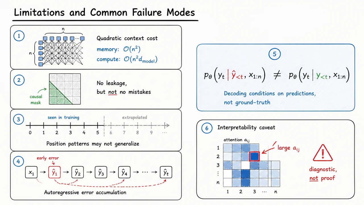
After looking at the limitations and failure modes, it is worth ending by stepping back from the many names Transformer models have acquired. “BERT-style,” “GPT-style,” “T5-style,” encoder-only, decoder-only, encoder-decoder: these are not fundamentally different mathematical species. They are different ways of wiring the same core operation, imposing different visibility constraints, and training against different probability factorizations.
The shared core is still scaled dot-product attention:
This equation is the common language of the architecture. Queries ask what information is needed, keys advertise what each position contains, and values carry the information to be mixed. The dot product implements content-based retrieval; the scale factor keeps logits from growing too large as the key dimension increases; and the additive mask determines which token-to-token communications are legal.
That last term, , is deceptively important. Much of the difference between Transformer variants comes not from changing attention itself, but from changing who is allowed to attend to whom. A padding mask prevents the model from treating artificial padding tokens as real content. A causal mask prevents position from looking at positions , preserving autoregressive generation. Cross-attention uses queries from one sequence and keys/values from another, allowing a decoder to retrieve information from an encoded source sequence.
Around this attention core, the standard Transformer block adds the same supporting machinery again and again: multi-head attention, a position-wise feed-forward network, residual connections, layer normalization, and some form of position information. Multi-head attention lets different subspaces implement different retrieval patterns. The feed-forward network transforms each token representation locally after communication. Residual paths stabilize optimization and preserve information across depth. Normalization controls activation scale and makes very deep stacks trainable. Positional encodings or embeddings break the permutation symmetry that pure self-attention would otherwise have.
So the most useful distinction among Transformer families is probabilistic rather than architectural.
An encoder-only Transformer uses bidirectional self-attention. Each token can attend to tokens on both its left and right, subject only to padding constraints. This makes it natural for classification, tagging, retrieval, and masked-token-style objectives where the model is allowed to build a contextual representation of the entire input. It does not directly define a left-to-right generative factorization unless one is added through the task design.
A decoder-only Transformer uses causal self-attention. Token may depend only on , so the model defines an autoregressive distribution
The usual maximum-likelihood training objective is
This factorization is what makes decoder-only models natural language generators: at inference time, we repeatedly sample or select the next token, append it to the context, and run the same conditional distribution again.
An encoder-decoder Transformer combines both patterns. The encoder reads the full source sequence bidirectionally. The decoder generates the target sequence causally, while also using cross-attention to retrieve source-side information from the encoder. Its probability model is
with objective
This is the classical sequence-to-sequence setting: translation, summarization, speech recognition, structured generation, and any task where an output sequence is generated conditionally on an input sequence.
The key takeaway is that architecture, mask, and objective must agree. If a model is trained with a causal mask, it can be used autoregressively without leaking future information. If a model has bidirectional attention, it can produce rich contextual embeddings, but it cannot be naively sampled left-to-right as though it had learned . If a model uses cross-attention, it explicitly separates source representation from target generation. Many practical failures come from confusing these regimes: using the wrong mask, training with one visibility pattern and decoding with another, or assuming that all Transformer outputs correspond to the same kind of probability distribution.
A compact way to remember the whole lecture is:
The visual summary below consolidates this unification. The attention equation sits at the top because it is the invariant mechanism. Beneath it, the three major Transformer forms differ mainly in their attention pattern, mask, modeled distribution, and loss. Read the table horizontally: each row is a coherent contract between visibility, probability, and training.
The footer slogan is also the right mental model to leave with: Transformers are differentiable content-addressable communication layers plus position information, stacked deeply and trained by maximum likelihood. Once that is clear, the apparent diversity of Transformer architectures becomes much easier to organize.
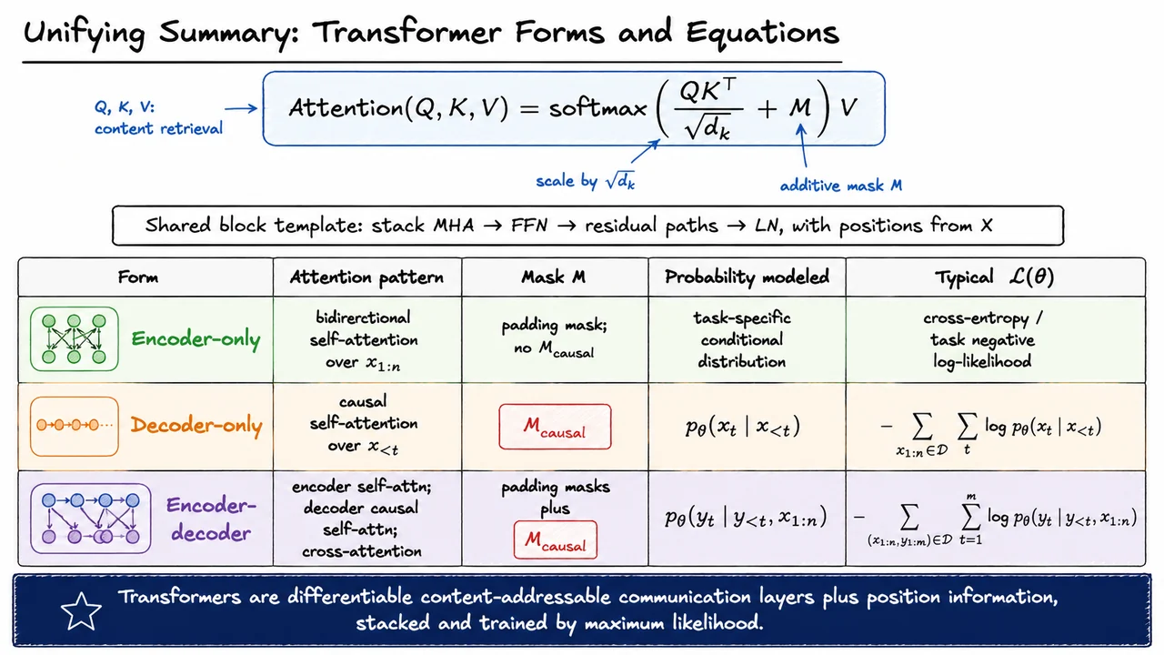
Before we talk about attention, it is worth naming the problem it was designed to solve. A sequence model is not merely a machine that consumes tokens in order; it is a machine that must route information between positions. If token matters for predicting something at position , the architecture needs a reliable computational path from to . The central question is: how long, fragile, and sequential is that path?
Many important tasks can be written abstractly as sequence-to-sequence mappings,
where the input and output lengths may differ. Translation maps a sentence in one language to a sentence in another. Summarization maps a long document to a shorter text. Code generation maps a prompt or partial program to a completed program. Even when the output is not explicitly a separate sequence, language modeling has the same flavor: at each position , the model predicts the next token from the previous context,
This notation hides the hard part. The conditioning set may be large, but not every previous token is equally relevant. A model predicting the verb in a sentence may need to find the true subject many tokens earlier. A model completing code may need to remember an opening bracket, variable declaration, or function signature hundreds or thousands of tokens back. A translation model may need to align a word near the end of the source sentence with a word near the beginning of the target sentence. In all cases, sequence modeling requires selective communication between positions.
Classical recurrent neural networks handle this by passing information through a hidden state:
This is elegant because it respects temporal order and can in principle summarize everything seen so far. But it creates a narrow communication channel. If information from is needed at , it must survive repeated transformations through
The number of computational steps between the two positions grows with their distance, roughly . Gradients must also travel through this same chain during training. Gating mechanisms such as LSTMs and GRUs reduce the damage, but they do not remove the fundamental bottleneck: distant tokens communicate through a long sequential path.
Convolutional sequence models improve parallelism because all positions in a layer can be processed simultaneously. However, local convolutions have their own routing problem. A kernel of small width only mixes nearby tokens in one layer, so long-range interaction requires stacking many layers. Dilated convolutions shorten the path, but the architecture still imposes a predefined communication pattern. Whether two positions can exchange information efficiently depends on the convolutional design rather than on the content of the sequence itself.
This suggests three desiderata for a strong sequence architecture:
The key insight behind Transformers is to replace sequential recurrence with learned content-based communication. Instead of requiring information to move one step at a time through a hidden state chain, each position can directly ask: which other positions contain information useful for me? Attention implements this as a differentiable retrieval mechanism. Positions produce queries, keys, and values; similarity between queries and keys determines where information flows. The route is not hard-coded by distance or adjacency. It is learned from content.
This matters because many sequence dependencies are sparse but not local. A token may need its immediate neighbors for syntax, a faraway noun for agreement, and an even farther definition for semantic interpretation. Architectures based only on local or sequential propagation must repeatedly carry all potentially useful information forward. Attention instead allows the model to create direct edges between relevant positions, making the effective path length between and very short.
The visual below condenses this bottleneck into a single picture: an input sequence , an output sequence , and the central challenge of connecting distant but relevant positions. The faint recurrent chain represents the older strategy: information moves through many local transitions, producing a long path . The highlighted long-range arrow represents the dependency we actually care about.
The same visual also previews the Transformer solution. Rather than relying only on neighboring steps, positions exchange information through learned, content-based links. Those direct communication paths are the conceptual bridge from traditional sequence models to attention: the model still respects sequence structure, but it no longer forces all information to travel through a narrow sequential corridor.
The bottleneck is easiest to dismiss when we talk about it abstractly: “long-range dependency” sounds like a rare linguistic edge case. But the problem appears in one of the most ordinary tasks a language model performs: choosing the next word. Even a short sentence prefix can force the model to decide whether to trust nearby evidence or route information from a more distant but grammatically relevant token.
Consider the prefix
The next word should be “are”, not “is”:
The grammatical subject is keys, which is plural. But by the time the model reaches the prediction position, the most recent nouns are cabinet and door, both singular. A model that overweights local context may be tempted by the nearby phrase “near the door” and predict a singular verb:
This is the long-range agreement trap. The correct prediction depends not on the closest noun, but on the noun that structurally controls the verb. In the prefix,
is the controller, while
are distractors. The model must learn a conditional preference of the form
The important point is that this inequality is not merely about memorizing that “keys” often goes with “are.” It requires the model to identify which earlier token is relevant for this prediction. The phrase contains multiple nouns, and the nearest ones are misleading. Sequential distance and grammatical relevance have come apart.
This exposes a weakness of purely local prediction. If the model primarily summarizes recent tokens, then the final phrase “near the door” dominates the representation near the prediction point. But the word door should not control the verb. It is embedded inside a prepositional phrase modifying cabinet, which itself is embedded inside another prepositional phrase modifying keys. The relevant dependency skips over these intervening tokens.
A good sequence model therefore needs a mechanism for content-based routing. Instead of asking, “Which token is closest to the current position?”, it should ask something more like:
For subject–verb agreement, the feature being routed is number: plural versus singular. In other examples, it might be entity identity, coreference, topic, tense, quotation state, or a variable binding. The general pattern is the same: the model must retrieve information by relevance, not by position alone.
This is one of the motivations for attention. Attention will eventually give us a differentiable way to compare the current prediction context against earlier token representations and assign high weight to the tokens whose content matters. The long-range token does not need to be compressed through every intermediate step with equal fidelity; it can be selected directly when it becomes useful.
The visual below condenses this failure case into a single next-token decision. The prefix is laid out as token boxes, with the blank prediction position at the end. The plural noun keys is far away but is the true controller of the verb, while cabinet and door are closer distractors. The central mistake to avoid is treating proximity as a proxy for relevance.
The probability inequality on the right states the learning target: the model should assign higher probability to “are” than to “is” given the whole prefix. That small inequality captures the larger architectural lesson: long-range dependencies require mechanisms that can route information by content relevance, not merely by sequential neighborhood.
The agreement trap from the previous section is not just a quirky linguistic example; it exposes a more general systems problem. A model must move information from some earlier position —where the relevant subject, entity, or condition appears—to a later position , where that information is needed to make a prediction. The intervening tokens may be syntactically plausible distractors, but semantically irrelevant. The question is: how many computational steps must the signal traverse before position can use what position knew?
For a recurrent model, the route is built into the architecture. Information at is first absorbed into a hidden state , then passed forward one position at a time:
This gives RNNs a useful inductive bias: nearby temporal continuity is natural, and the hidden state acts like a running summary. But the same design becomes a bottleneck for long-range dependencies. If and are far apart, then the representation of must survive many state updates, each of which may overwrite, compress, or distort it. Even if the model has gates, such as in an LSTM or GRU, the route is still sequential. The architecture can learn to preserve information, but it cannot avoid the fact that the information must pass through many intermediate states.
The training signal suffers from the same geometry. When a loss at position assigns credit to something that happened near , the relevant derivative contains a long product of Jacobians:
This product is the mathematical heart of the vanishing and exploding gradient problem. If the typical singular values of these Jacobians are smaller than one, the gradient decays exponentially with distance; if they are larger than one, it can blow up. Gating, normalization, careful initialization, and gradient clipping can make this more manageable, but they do not remove the long credit-assignment path. The model is still being asked to propagate both information and gradients through sequential transformations.
Convolutional sequence models attack the problem differently. Instead of carrying a hidden state from left to right, they update all positions in parallel using local windows. This is excellent for parallel training: every position in a layer can be computed at the same time. But locality introduces a different limitation. A token can only influence positions within the receptive field of the convolution, and that receptive field grows layer by layer. With a kernel of fixed width, distant positions require many layers before they can interact.
So CNNs trade the RNN’s sequential time bottleneck for a depth bottleneck. A sufficiently deep convolutional network can connect distant positions, and dilated convolutions can expand the receptive field faster, but the architecture still imposes a structured route through intermediate neighborhoods. Distant communication is possible only after repeated mixing. In practice, this means either many layers, large kernels, carefully chosen dilation schedules, or some combination of these. The model’s ability to relate and is mediated by architectural distance.
This is the motivation for attention as a new primitive. Instead of forcing information to travel through every intermediate hidden state, or to diffuse through local convolutional neighborhoods, we would like position to directly retrieve information from position when is relevant. In the idealized path-length sense, attention offers:
That statement does not mean attention is computationally free. Full self-attention over a sequence of length compares many pairs of positions, which introduces its own cost. Rather, the point is about communication distance: once the attention scores are computed, any position can incorporate information from any other position in a single layer. The burden shifts from “can the information survive the route?” to “can the model learn which positions matter?”
This shift is subtle but crucial. RNNs and CNNs bake in a strong notion of locality: information moves through adjacent time steps or nearby windows. Attention weakens that assumption and replaces it with content-based routing. If a verb at position needs the subject at position , the model can learn to assign high weight to that subject directly, even across many distractors. The resulting architecture is often easier to optimize for long-range dependencies because the forward information path and the backward credit-assignment path are both shorter.
The comparison can be summarized as follows:
The visual below condenses this argument into a side-by-side comparison. The recurrent row emphasizes the chain from to , while the gradient row highlights why that chain is also an optimization problem. The convolutional row captures receptive-field growth through stacked local windows. The attention row contrasts these with a direct connection from to , foregrounding the key design goal: reduce the path length for relevant interactions to .
Read the table not as saying that attention is universally cheaper or always better, but as isolating the architectural reason Transformers became compelling. They replace forced sequential or local communication with a differentiable mechanism for deciding who should talk to whom. That mechanism—attention as learned lookup—is the next object we will derive.
The previous discussion identified a common bottleneck behind both recurrence and convolution: routing information. If a token near the end of a sequence needs evidence from a token near the beginning, an RNN must carry that evidence through many recurrent steps, while a CNN must propagate it through many local receptive fields unless the network is made very deep or uses large kernels. The issue is not merely that long paths are inconvenient; long paths make learning fragile. Gradients, intermediate states, and local transformations all become part of the communication channel.
A more direct primitive would let each position ask: which other positions contain information useful for me right now? Instead of forcing information to move step by step through a fixed computational graph, we want every position to be able to retrieve relevant content from anywhere in the sequence in one operation. This is the motivation behind attention.
The simplest abstraction is a content-based lookup. Imagine that each position in a sequence stores some information in a vector , called a value vector. Now suppose position wants to update its representation. Rather than reading only its neighbor or the previous hidden state, position forms a weighted combination of all available values:
The coefficients are the attention weights. They say how much position retrieves from position . To make this retrieval behave like a soft selection, the weights are constrained to be nonnegative and sum to one:
These constraints make the retrieved vector a convex combination of the value vectors. Intuitively, position is not copying a single source exactly; it is averaging information from multiple sources, with more relevant positions receiving larger weights. This convex-mixture view is important because it gives attention a stable numerical interpretation: the output remains in the span of available information rather than becoming an unconstrained linear explosion.
A hard lookup would choose one position and return . That is useful in classical data structures, but it is awkward for gradient-based learning: a discrete choice is not smoothly differentiable with respect to the scores that produced it. Attention replaces that hard decision with a soft lookup. If the model is uncertain between two relevant tokens, it can assign weight to both. If training later reveals that one source was more useful, gradients can continuously shift probability mass toward it.
This also explains why attention is more than a memory trick. The weights should not be fixed by distance or position alone. They should depend on content compatibility: what the current position needs and what each candidate source offers. For example, in a translation model, a decoder position producing a verb may need to retrieve the subject from far away. In a language model, a pronoun may need to retrieve a compatible antecedent. The useful source is determined by meaning and context, not simply by being nearby.
There are a few subtle assumptions hidden in this primitive. First, the value vectors must contain information worth retrieving; attention can route information, but it cannot recover content that was never represented. Second, the weights must be produced by a learnable scoring mechanism that can compare position 's needs with position 's contents. Third, because the retrieved vector is a mixture, attention can sometimes blur information when many incompatible sources receive nontrivial weight. Later, scaled dot-product attention will address how to compute these weights effectively and how to keep the scoring distribution numerically well behaved.
The key conceptual shift is therefore:
The visual below condenses this idea into a single routing picture. The sequence positions each hold a value vector . For a target position , arrows from all positions represent possible communication channels, and their thickness represents the learned attention weights . The output at position is not one copied vector, but the soft mixture .
This compact diagram is the bridge from motivation to mechanism. We have not yet specified how the weights are computed—that will require embeddings, queries, keys, values, and scaling—but we have specified the primitive we want: differentiable, content-based retrieval over a sequence.
Now that we have framed attention as a kind of differentiable lookup, we need to answer a deceptively basic question: what exactly are we looking up with? A Transformer cannot operate directly on raw symbols like "cat", "sat", or ".". Those symbols are discrete vocabulary items; they have no geometry, no dot products, no notion of similarity that a neural network can manipulate smoothly. Before attention can compare one token to another, every token must be represented as a vector in a shared continuous space.
The first ingredient is the token embedding table. If the vocabulary is and the model width is , we learn a matrix
Each row of is the learned vector representation of one vocabulary item. For a token , the embedding lookup returns
This is often described as a “lookup,” but it is still part of the differentiable model: the selected embedding vector participates in the forward computation, receives gradients during backpropagation, and is updated during training. Over time, the model learns an embedding geometry in which useful distinctions for prediction become linearly accessible to later layers.
However, token identity alone is not enough. The sequence
does not mean the same thing as
If we gave self-attention only the multiset of token embeddings , then the model would know which tokens appeared, but not where they appeared. This is especially important because vanilla self-attention, unlike recurrence or convolution, does not inherently process tokens left-to-right or through local neighborhoods. Its core operation compares rows of a matrix to other rows of the same matrix. Without additional positional information, that operation is naturally permutation-equivariant: reorder the input rows, and the corresponding outputs reorder in the same way.
So Transformers add a second vector to each token representation: a position vector. For a maximum sequence length , we can represent these position vectors as rows of a matrix
The vector tells the model that this row corresponds to position . In the original Transformer, these were sinusoidal encodings; in many modern models, they are learned or replaced with relative/rotary variants. But the conceptual role is the same: position information must enter the representation somehow, because attention by itself only sees a set of content vectors.
The simplest absolute-position construction is additive. For each token , we combine “what token is here” with “where it is”:
Stacking these row vectors gives the Transformer’s input matrix
This matrix is the object that will be projected into queries, keys, and values in the next step. Each row is one token position, and each row lives in the same -dimensional space.
The addition is worth pausing over. We are not concatenating token and position into a larger vector; we are superimposing them in the same model dimension. That means the model must learn to use the shared coordinates to encode both lexical/content information and positional information. This works because the subsequent linear projections can learn directions that respond to content, position, or mixtures of the two. But it also encodes an assumption: the model width must be large enough to carry all the information the network needs.
A useful way to think about a row of is:
That last phrase is crucial. Attention will not retrieve information from isolated word types; it will retrieve from contextualizable slots in a sequence. The same token can appear in two positions and begin with the same embedding, but after adding different 's, the initial vectors are no longer identical. This allows later attention layers to distinguish, for example, the first occurrence of a word from the second.
There is also an important failure mode hiding here. If we omitted , then a self-attention layer with shared projections would not know whether a token came first, last, or somewhere in the middle. It could still compare content, but it would lack sequence order. For tasks where order matters—and almost all language tasks do—that is a severe limitation. Positional information is therefore not a decorative add-on; it is what turns a bag of token vectors into a sequence representation.
The visual below compactly summarizes this construction as a pipeline: raw tokens are mapped through the embedding table , position rows are supplied from , and corresponding vectors are added row by row to form . The key idea to look for is that the Transformer input is not “just embeddings,” but embeddings plus positions.
It also foreshadows the next step. Once has been assembled, attention can create queries, keys, and values by learned linear projections. In other words, the differentiable retrieval mechanism we want is built on top of this matrix: each row of is now a content-and-position-aware record that attention can compare, weight, and combine.
Once tokens have been turned into vectors, we have a useful representation at every sequence position—but each position is still mostly carrying local information: “what token am I?” and “where am I?” The next problem is how one position can use information stored at other positions. If the word “it” appears late in a sentence, its representation may need to borrow meaning from a noun many tokens earlier. If a code variable is used after several lines, its current representation should be able to retrieve the earlier definition.
The key idea of attention is to make this retrieval differentiable. Instead of choosing exactly one previous token or one memory slot, a position forms a weighted average over many stored vectors. For a particular query position , suppose every position stores some vector , called a value. The output representation at position is
This is the central retrieval equation. The output is not copied from a single location; it is blended from all available values. The coefficient tells us how much position retrieves from position .
For this weighted average to behave like retrieval, the weights should be nonnegative and should sum to one:
So lies in the convex hull of the value vectors. Intuitively, attention says: “construct the new representation by mixing stored content, with mixture proportions determined by relevance.” This is a softer and more trainable version of lookup in a dictionary or memory table.
The weights themselves come from compatibility scores , where measures how relevant position is to position . We convert these arbitrary real-valued scores into normalized weights using a softmax over the retrievable positions:
The denominator is important: for a fixed retrieving position , the model compares all candidate positions against one another. Attention is therefore relative: a token receives high weight not merely because its score is large in isolation, but because its score is large compared with the alternatives in the same row.
This row-wise normalization has several consequences. First, attention weights are easy to interpret as a distribution over source positions. Second, the operation is differentiable end-to-end, so learning can adjust both the scoring mechanism and the stored value vectors. Third, the softmax introduces competition: increasing tends to decrease the mass assigned elsewhere. That competition is part of what makes attention behave like selective retrieval rather than an unstructured sum.
There is also a subtle but crucial separation here: scoring and content are conceptually different. The score determines where to look; the value determines what information is retrieved once we look there. This distinction will become central when we introduce queries, keys, and values. For now, it is enough to notice that the vector used to decide relevance need not be identical to the vector whose information is ultimately copied into the output.
Stacking the outputs for all positions gives the matrix form. Let contain the value vectors row by row, and let contain the attention weights, with row holding the distribution . Then
This equation is compact but powerful. Each row of is a weighted average of the rows of . The matrix is not just a generic linear map; it is row-stochastic, meaning each row is a probability distribution. Attention is therefore a structured, data-dependent linear combination of stored representations.
The visual below condenses this idea into two complementary views. On the algebraic side, it emphasizes the chain from scores , to softmax-normalized weights , to retrieved output . On the retrieval side, one position sends different-strength connections to several stored values , and those weighted contributions merge into the output vector.
The most important takeaway is that attention is not yet “magic Transformer machinery.” At this stage, it is simply weighted differentiable retrieval. The model computes relevance scores, normalizes them into a distribution, and uses that distribution to average content vectors. The next step is to specify how the scores are produced—and that is where queries, keys, and values enter.
The weighted-retrieval view gives us a useful abstraction: once we have an attention matrix , producing outputs is just
a weighted average of “retrievable” vectors. But this leaves an important question unresolved: where do the weights in come from, and what exactly are we averaging? If the same representation of a token is used both to decide whether it is relevant and to supply the content returned, the model is forced to entangle two different roles. Transformers avoid this by separating matching from retrieval.
The key move is to project each input position into three learned spaces:
Here is the sequence of contextual token representations: positions, each represented by a -dimensional vector. The learned projection matrices have shapes
so the resulting matrices are
Conceptually, each row of these matrices plays a different role. The row of is the query for position : it represents what that position is looking for. The row of is the key for position : it represents how position advertises itself for matching. The row of is the value for position : it is the information returned if some other position decides to attend to .
This distinction is subtle but central. A word may need to be matched according to one set of features, while returning a different set of features once selected. For example, a pronoun might look for a compatible noun phrase using syntactic and semantic cues encoded in queries and keys, but the information retrieved from the noun phrase might include number, gender, entity identity, or broader contextual meaning encoded in the value vector. The model should not have to use the same coordinates for all of these purposes.
In self-attention, all three matrices are projected from the same input . That is why the mechanism is “self”: every position can attend to other positions in the same sequence. But the projections are different, so “same source” does not mean “same representation.” The model learns three views of each token:
This separation also explains why attention is more flexible than a fixed similarity computation on raw embeddings. If we compared rows of directly, the notion of relevance would be tied to whatever features happen to be present in the model representation. By learning and , the Transformer learns a task-specific compatibility space. By learning , it separately learns what content should flow forward after compatibility has been determined.
There are also important dimensional choices hidden in these equations. The query and key dimensions must match, because they will be compared to produce attention scores; hence both live in . The value dimension , however, need not equal , because values are not used for matching in the same way. They are aggregated after the attention weights have already been computed. In practice, architectures often choose convenient equal dimensions, especially inside multi-head attention, but the mathematical roles remain distinct.
A useful way to think about the full computation is:
So and answer the question, “Which positions should interact, and how strongly?” while answers, “What information should be passed along once that interaction is chosen?” This is the bridge from abstract weighted retrieval to the concrete attention mechanism used in Transformers.
The visual below compactly summarizes this decomposition. A single input matrix branches into three learned projections: , , and . The parallel arrows emphasize that these are not three different input sequences, but three learned views of the same sequence. Highlighting individual rows , , and reinforces the position-wise interpretation: one position asks, another position matches, and the matched position returns content.
The faded continuation toward is also important. It reminds us that values are still the objects being averaged, as in weighted retrieval, but the weights will now be produced by comparing queries and keys. This separation is the conceptual step that makes scaled dot-product attention possible: first learn what to match, then learn what to return.
With queries, keys, and values in place, the next question is: how should a query decide which keys are relevant? We have already separated “what I am looking for” () from “what each position offers as an address” () and “what content I can retrieve” (). Attention now needs a compatibility function that turns each query–key pair into a scalar score.
The simplest and most important choice is the dot product:
This score is large when and point in compatible directions. Geometrically, the dot product rewards alignment: if two vectors have similar directions, their inner product is positive and large; if they are orthogonal, it is near zero; if they point in opposing directions, it can be negative. In attention, this means position assigns a high raw score to position when the learned query at matches the learned key at .
There is a subtle but important assumption here: the learned projections that produce and are free to shape the space in which “matching” happens. We are not comparing raw token embeddings directly. Instead, the model learns a coordinate system where certain directions correspond to useful retrieval patterns: syntactic agreement, coreference, local continuation, delimiter matching, or any other relation that helps the task. The dot product is simple, but the learned projections make it expressive.
For a sequence of length , every query position compares itself to every key position. If we stack the query vectors into a matrix
and the key vectors into
then all pairwise dot products appear at once in the matrix product
This is one of the central computational facts behind Transformers: attention is vectorized all-pairs comparison. Instead of iterating through the sequence recurrently, each position can compare against every other position in a single batched matrix multiplication. That is why attention is so well matched to modern accelerators: the communication pattern is dense, but it is expressed as large linear algebra operations.
The raw score matrix is not yet a retrieval distribution. Each row contains the scores for one query position against all possible source positions . To turn these scores into weights, we apply a row-wise softmax:
Here can be read as “how much position attends to position .” The rows of sum to one, so each query forms a weighted average over values. The retrieved output vectors are then
This is the full dot-product attention pattern before scaling and masking: compare queries to keys, normalize scores into attention weights, then use those weights to average values.
It is worth emphasizing what this buys us. A recurrent model must pass information through a chain of hidden states, so distant positions interact through many sequential steps. A convolutional model needs either large kernels or many layers to connect distant tokens. Dot-product attention, by contrast, gives every position a direct path to every other position in one layer. The cost is that the score matrix has entries, so dense self-attention is powerful but expensive for long sequences.
There are also important failure modes hidden in this compact formula:
The next section will address the first of these issues directly: why the raw dot product is divided by . For now, the key idea is that dot-product attention is not mysterious. It is a learned content-addressable lookup system implemented as matrix multiplication.
The visual below consolidates this flow. On the left, the equations isolate the three conceptual steps: define a pairwise compatibility score, vectorize all scores as , and retrieve values using softmax-normalized weights. On the right, the matrix pipeline makes the same idea operational: rows of meet rows of through , producing a score grid whose cell is exactly .
The important thing to notice is the dense all-pairs communication pattern. Every query row has access to every key column before the softmax chooses how much value information to retrieve. That single pattern,
is the algebraic heart of attention.
Having introduced dot products as a natural compatibility score between a query and a key, there is one more detail that looks like a harmless implementation trick but is actually crucial for stable learning: Transformer attention does not use directly. It uses a scaled dot product.
The raw score between query and key is
At first glance, this seems perfectly reasonable. If the query and key point in similar directions, the dot product is large; if they are unrelated or opposed, it is small or negative. But the magnitude of this score depends not only on semantic alignment. It also depends on the key/query dimension . As grows, the dot product accumulates more random terms, so even unrelated vectors can produce scores with increasingly large variance.
A simple initialization-style calculation makes the issue visible. Suppose the components of and are independent, centered, and normalized:
These assumptions are not meant to describe every trained Transformer exactly. They are a controlled approximation: before learning has shaped the representations too much, and under common normalization/initialization schemes, it is reasonable to ask what scale the scores would have if the components behaved like independent unit-variance random variables. The goal is to prevent the architecture itself from injecting an undesirable scale factor.
For one coordinate product, independence gives
and
So each coordinate contributes a unit-variance random term to the dot product. Since the full score sums such terms, the variance grows linearly:
Equivalently, the standard deviation of the raw dot product grows like . This is the key point: increasing the representation dimension makes the scores larger in magnitude even when there is no stronger evidence of relevance.
That matters because attention does not use the scores directly; it passes them through a softmax. The softmax is sensitive to scale. If its inputs are small or moderate, it can assign a graded distribution over many keys. But if one logit is much larger than the others, the output becomes nearly one-hot:
Large score variance therefore pushes attention into a saturated regime. One key receives almost all the probability mass, the others receive almost none, and the gradients through the softmax become less informative. The model may still train, but optimization becomes unnecessarily brittle: early random score differences can dominate attention before the network has learned meaningful retrieval patterns.
The fix is to normalize the score by its typical standard deviation. Since
we compute attention using
This does not change the basic content-based retrieval story. Queries still compare themselves to keys, and values are still averaged according to the resulting attention weights. The scaling only keeps the logits in a numerically and statistically reasonable range as the key/query dimension changes.
A useful way to read the result is:
The visual below condenses this argument into two complementary views. On one side, the variance derivation tracks how the score accumulates independent unit-variance products, ending in the highlighted conclusion . On the other side, the same phenomenon is shown operationally: unscaled scores become tall and uneven, producing a sharply peaked attention row, while scaled scores produce a smoother, more stable distribution.
The important takeaway is not that attention should always be diffuse. A trained Transformer can and often should place highly concentrated attention when the data calls for it. The point is that this concentration should be learned, not forced by the dimensionality of the dot product. Scaling by makes dot-product attention behave consistently across dimensions, giving the softmax a well-conditioned set of logits to work with.
After controlling the scale of the dot products, the next issue is not how strongly one token should attend to another, but whether that link should exist at all. Attention, by default, is completely content-driven: every query compares itself with every key, and the softmax turns those comparisons into a probability distribution over all value vectors. That is powerful, but it is also too permissive. Some attention links are structurally invalid regardless of content.
The mechanism for enforcing these hard constraints is an attention mask. Starting from the scaled attention logits,
we add a mask matrix before applying the row-wise softmax:
Here has the same row-column structure as the attention score matrix: rows correspond to query positions, columns correspond to key/value positions. The key idea is that masking happens at the logit level, before normalization. This matters because the softmax is sensitive to additive changes in logits: setting a logit to makes its exponent exactly zero.
Concretely, for query position and key/value position ,
means the link is allowed. The original scaled dot-product score is unchanged, so the model may assign attention mass to if the content match is strong. In contrast,
means the link is forbidden. Since
the corresponding softmax weight becomes
Therefore contributes nothing to the output vector at query position , no matter how compatible and might have been.
This is a hard structural constraint, not a learned preference. The model is not being encouraged to avoid certain links; it is made mathematically impossible for those links to carry information. In actual implementations, is often represented by a very large negative number for numerical reasons, but the intended operation is the same: after softmax, the masked probability is zero or effectively zero.
The most important example is causal self-attention, used in autoregressive language modeling. When predicting token , the model may use tokens at positions , but it must not look ahead to future positions . Otherwise, training would leak the answer: the representation for an earlier token could directly depend on later tokens that should not yet be known during generation.
The causal mask is therefore
This gives a lower-triangular pattern, including the diagonal. Position can attend only to itself, position can attend to positions and , and so on. The diagonal is usually allowed because the representation at a position may use the token currently being processed when computing hidden states for next-token prediction; what is forbidden is access to future positions.
The same additive-mask abstraction covers several different situations:
A subtle but important point is that masks operate independently of the learned parameters. The matrices , , and are still produced by learned projections, and the model still decides among allowed links using content similarity. The mask simply defines the set of possible routes through which information may flow. In graph terms, attention learns edge weights, while the mask determines which edges are present.
The visual below condenses this into two complementary views. On the left, the mask appears exactly where it belongs mathematically: added to the scaled dot-product logits before the softmax. The two cases and then become easy to interpret as “keep this candidate link” versus “force its attention weight to zero.”
On the right, the causal mask is represented as a triangular matrix. The allowed region contains zeros, while the forbidden future region contains . After the row-wise softmax, that forbidden upper triangle disappears from the attention matrix : future value vectors cannot contribute to earlier query positions. This is the small algebraic trick that makes Transformer attention compatible with autoregressive sequence modeling.
After introducing masks, it is tempting to think of attention as a graph over sequence positions: some token positions may attend to others, and masking removes selected edges. But before we add masks—or positional encodings—there is a deeper fact hiding in plain sight: content-only self-attention does not know what a sequence order is. It sees an matrix as a collection of row vectors and computes interactions among those rows, but nothing in the vanilla attention formula says that row comes before row , or that row is special because it is first.
Let , where each row is a token representation. A single-head self-attention layer without positional information computes
and then
The softmax is applied row-wise: each query row produces a probability distribution over all key rows, and then forms a weighted average of value rows. This is content-based retrieval: each token asks, “which other token vectors are relevant to me?” The important subtlety is that relevance is computed only through dot products of learned projections. There is no term involving the integer index , no sinusoidal or learned positional vector , and no causal or padding mask that distinguishes allowed from disallowed positions.
Now consider a permutation matrix . Multiplying on the left by simply reorders the rows of . For example, if contains token vectors in one order, then contains the same token vectors in a different order. The theorem says that self-attention commutes with this reordering:
That property is called permutation equivariance. It is not invariance: the output does change when the input is permuted. But it changes in exactly the same way—the output rows are permuted by the same . In other words, content-only self-attention treats the input as an unordered set of token vectors, while still returning one output vector per input token.
The algebra is short but instructive. If we permute the input rows, the projected queries, keys, and values become
The new attention score matrix is
So the score matrix is not arbitrary; it is the original score matrix with both rows and columns permuted. Rows are permuted because the queries have been reordered, and columns are permuted because the keys have been reordered. The scaling by does not affect this symmetry.
The only slightly delicate step is the row-wise softmax. For any score matrix ,
This holds because permuting a row before applying softmax simply permutes the resulting probabilities in the same way, and permuting the collection of rows also just reorders the row-wise outputs. Applying this to
we get
Multiplying by the permuted values cancels the inner permutation:
Substituting back , , and , the theorem is exactly
This result matters because language is not merely a bag of token embeddings. The sentences “dog bites man” and “man bites dog” contain the same token set but mean different things. A Transformer without positional information cannot distinguish these two sequences by order alone. If the token embeddings are identical and only their rows are rearranged, the layer can only rearrange its outputs correspondingly. It has no intrinsic mechanism for representing “before,” “after,” “nearby,” or “first.”
There are also useful boundary cases to keep in mind. The equivariance statement assumes no positional encoding , no mask , and no position-dependent biases. Adding absolute positional embeddings breaks the symmetry because row receives information tied to index . Adding a causal mask also breaks full permutation equivariance because the mask privileges the left-to-right order. By contrast, operations applied identically to every row—such as a shared feed-forward network, residual addition, or layer normalization over features—typically preserve permutation equivariance. The symmetry is broken only when the model is given some information that distinguishes positions.
The visual below compactly summarizes the theorem as a commuting diagram: one path permutes the input rows first and then applies self-attention, while the other applies self-attention first and then permutes the output rows. The equality says these paths arrive at the same result. That is the operational meaning of permutation equivariance.
The equation in the theorem box is the algebraic version of the same story. The orange terms track row permutations, the blue softmax block tracks how attention weights reorder consistently, and the green value block reminds us that the final weighted sums are attached to the same permuted rows. The important takeaway is simple but profound: without positions or masks, self-attention is a powerful content-retrieval mechanism, but not yet a sequence model in the ordered sense.
The equivariance result is useful precisely because it tells us what self-attention cannot know by itself. If the inputs are just token embeddings, self-attention treats the sequence as a set of content vectors with indices attached only externally. It can route information based on what appears, but not intrinsically on where it appears. That is elegant from a symmetry perspective, but disastrous for language, programs, music, genomes, and essentially every sequence domain where order changes meaning.
For example, the two strings “the dog bit the man” and “the man bit the dog” contain almost the same multiset of token identities. A content-only self-attention layer can produce correspondingly permuted representations, but it has no built-in reason to distinguish subject position from object position. The problem is not that attention is weak; the problem is that attention is too symmetric. We must deliberately break permutation symmetry by injecting positional information.
The standard Transformer does this by replacing each token embedding with a position-aware input representation such as
where is a vector associated with position . Now the attention mechanism no longer receives just “the embedding for this word”; it receives “the embedding for this word at this location.” The dot products used to compute attention can depend on token identity, position, and interactions between the two. In other words, attention remains content-based retrieval, but the content being retrieved has been enriched with location.
There are several ways to choose the positional signal. The original Transformer used sinusoidal positional encodings, where each coordinate varies periodically with position at a different frequency. Learned absolute embeddings are also common: the model simply learns a table . More recent architectures often use relative position biases or rotary positional embeddings, which modify the attention scores or query/key geometry so that the model reasons more directly about offsets like “three tokens ago” rather than absolute coordinates like “position 57.”
These choices differ in what generalization they encourage:
A subtle point is that masking is not a full substitute for positional encoding. A causal mask does introduce an ordering constraint: token cannot attend to future tokens . But without positional information, the model still has limited ability to distinguish different permutations of the visible prefix. The mask says “you may look backward,” but it does not fully tell the model which earlier token was first, second, or adjacent in a content-independent way. For sequence modeling, causality and position solve different problems: causality prevents information leakage, while positional encoding gives the model a coordinate system.
This also explains why positional information matters even in encoder-only models, where there is no causal mask. In a bidirectional encoder, every token can attend to every other token. Without positions, the representation of a sentence is equivariant to arbitrary reordering. A downstream classifier might collapse those token representations into something nearly permutation-invariant, making word order even harder to recover. Positional encodings give the encoder a way to represent syntactic roles, local neighborhoods, phrase boundaries, and long-range dependencies as structured relations rather than unordered co-occurrences.
The visual summary for this idea should be read as a symmetry-breaking story: content-only self-attention preserves permutation structure, while adding positional signals turns a bag-like collection of embeddings into an ordered sequence. Once token and position information are combined, attention can still retrieve by similarity, but similarity is now computed in a space where “same word in a different place” can mean something different.
This sets up the next architectural refinement. After we give the model a notion of position, a single attention operation still represents only one retrieval pattern at a time. In practice, different relationships matter simultaneously: nearby syntax, long-range agreement, delimiter matching, coreference, copying, and positional offsets. Multi-head attention will let the model learn several such retrieval subspaces in parallel.
Before assembling a full Transformer block, it is worth pausing on the attention mechanism itself. A single scaled dot-product attention layer already gives us a powerful content-addressable retrieval operation: each token forms a query, compares it against all keys, and uses the resulting weights to average the corresponding values. But one attention distribution is still only one way of asking, “What information should this token retrieve from the sequence?”
The central idea of multi-head attention is that a token may need to retrieve several different kinds of evidence at once. In language, for example, a word might need nearby syntactic context, a long-range subject for agreement, a previous mention for coreference, and a delimiter or boundary token for structure. These are not necessarily well represented by a single similarity function over one query-key space. Multi-head attention addresses this by running several attention mechanisms in parallel, each with its own learned projections.
Given an input sequence representation , each head learns separate projection matrices
These produce head-specific queries, keys, and values:
The head then performs the same scaled dot-product attention operation we have already developed:
The mask plays the same role as before: it can forbid attention to certain positions, such as future tokens in causal decoding or padding tokens in batched training. The scaling by also remains essential, because each head computes dot products in its own key/query dimension . Without scaling, the logits can grow too large in magnitude as increases, causing the softmax to become overly peaked and gradients to become less useful.
The important change is not the formula inside one head; it is the fact that each head has its own learned retrieval subspace. One head might learn projections where query-key similarity emphasizes syntactic adjacency. Another might emphasize semantic similarity. Another might specialize in positional or delimiter-like patterns. This specialization is not manually assigned; it emerges because the model can reduce training loss by distributing different retrieval behaviors across heads.
After computing all heads in parallel, their outputs are concatenated:
This concatenated representation contains multiple retrieved views of the sequence at each token position. A final learned output projection then mixes these views back into the model dimension:
This final projection is easy to underestimate. Concatenation alone would merely place the heads side by side. The output matrix lets the model form learned combinations across heads: it can amplify, suppress, or blend information retrieved by different attention patterns. In other words, multi-head attention is not just “several attentions in parallel”; it is parallel retrieval followed by a learned recombination step.
A common implementation choice is to keep the total compute roughly comparable to a single large attention layer by splitting the model dimension across heads. For example, if the model width is and there are heads, one often uses
Then each head is narrower, but there are more of them. This gives the model multiple attention patterns without multiplying the representation size before the output projection. The trade-off is that each individual head has lower dimensional capacity, while the collection of heads has greater diversity in possible retrieval behavior.
There are also subtle failure modes. Heads are not guaranteed to become neatly interpretable modules such as “syntax head” or “coreference head.” Some heads may be redundant, diffuse, or useful only in combination with others. In practice, attention patterns are informative but not always faithful explanations of model behavior. Still, the architectural bias matters: by giving the model several independent query-key-value projections, multi-head attention makes it easier to represent multiple relational structures simultaneously.
The visual below compactly organizes this computation from left to right. The same input fans out into several parallel lanes, one per head. Each lane applies its own , , and projections, performs masked scaled dot-product attention, and emits a head-specific retrieved representation. The different colors emphasize that these heads are not copies of one another; they are separate learned retrieval mechanisms operating in distinct subspaces.
On the right side, the heads are gathered by concatenation and passed through , which mixes them back into a single output representation . This is the key structural pattern to remember before moving to the rest of the Transformer block: parallel attention heads create multiple retrieved views, and the output projection integrates those views into the next token representation.
After multi-head attention has gathered information from different positions and different representation subspaces, the Transformer still needs a way to compute new features from the resulting token vectors. Attention is excellent at routing and mixing information across the sequence, but the weighted sums it produces are still largely linear combinations of value vectors. To make each token representation more expressive, every Transformer block follows attention with a position-wise feed-forward network.
The phrase position-wise is important. Suppose the block input is a matrix
where row is the representation of token position , already combining token identity and positional information. After multi-head attention, each row has had the opportunity to receive information from other rows. The feed-forward layer then applies the same nonlinear map to each row independently:
Here are shared across all positions, and is a pointwise nonlinearity such as ReLU or GELU. In modern Transformers, GELU-like activations are common, but the architectural idea is not tied to one particular choice.
A useful mental model is that attention answers the question: Which other positions should this token read from? The feed-forward network answers a different question: Given the information now stored in this token vector, how should we transform its features? These are complementary operations:
This independence means there is no communication between positions inside the FFN itself. If position affects position , that influence must have already been routed through attention or must happen in a later attention layer. The FFN is therefore not a replacement for attention; it is the nonlinear feature processor that acts after attention has assembled a useful local representation at each position.
The standard Transformer FFN has a characteristic expand-and-compress shape:
The first linear map projects each token vector into a wider hidden space of dimension . The activation introduces nonlinearity, allowing the model to form feature interactions that cannot be represented by attention’s weighted averaging alone. The second linear map compresses the representation back to , so the output can be passed cleanly to the next sublayer in the block.
This expansion matters. If the FFN were only a single linear map from to , then it would add limited expressive power, especially when surrounded by other linear projections. The intermediate width gives the model a larger workspace for computing token-wise features: detecting patterns, gating dimensions, composing semantic attributes, or re-encoding information gathered from attention. In many Transformer configurations, is several times larger than , making the FFN a major contributor to both parameter count and computation.
There is a subtle but important symmetry here. Because the same FFN parameters are applied to every row, the operation is shared over sequence length. The model does not learn one feed-forward map for the first token, another for the second token, and so on. Instead, positional differences are represented in the input vectors themselves, while the transformation rule remains the same everywhere. This sharing is one reason Transformers can process variable-length sequences: the FFN does not depend on a fixed sequence length .
Equivalently, we can view the FFN as a tiny multilayer perceptron applied in parallel to all token positions. In matrix form, ignoring broadcasting details for the biases, this is
but this compact expression can hide the crucial fact that row is transformed without directly reading row . The matrix notation is efficient; the row-wise interpretation is the architectural insight.
The visual below condenses this idea into a left-to-right pipeline. Each row vector enters an identical two-layer nonlinear transformation: expansion by , activation by , and compression by . The parallel lanes emphasize that there are no arrows between positions inside the FFN.
The shared-weight annotation is just as important as the lanes themselves. It reminds us that the FFN is independent across rows but not separately parameterized across rows. The same learned map is reused at every position, turning attention’s cross-token communication into richer per-token features before the block moves on to residual connections and normalization.
After adding the position-wise feed-forward network, we now have the two computational ingredients that make up a Transformer block: multi-head attention for token-to-token interaction, and an MLP/FFN for per-token nonlinear transformation. But simply stacking these transformations naively is usually unstable. Deep networks need a way to preserve information, keep gradients healthy, and prevent activations from drifting into poorly scaled regimes.
This is where the Transformer block becomes more than “attention followed by an MLP.” Each major sublayer is wrapped with three stabilizing mechanisms:
In the original Transformer formulation, these are arranged in a post-normalization pattern. For an input sequence representation , the attention sublayer produces an intermediate representation
Then the feed-forward sublayer is applied with the same wrapper:
The residual addition is not just a convenience. It gives the block a short identity route through depth. If the attention or feed-forward transformation is initially unhelpful, the model can still pass forward something close to the original representation. This matters because deep Transformers are trained by gradient descent: without residual paths, every layer would have to learn both how to preserve useful information and how to modify it. With residual paths, a sublayer can instead learn a correction or update to the current representation.
A useful way to think about one wrapped sublayer is
Attention contributes a context-dependent update, while the FFN contributes a token-wise nonlinear update. The residual path ensures that these updates are added to an existing representation rather than replacing it entirely. This “incremental refinement” viewpoint is one reason very deep residual architectures are trainable.
Dropout is placed on the sublayer output before the residual addition. During training, this randomly removes parts of the proposed update. The identity path remains intact, so dropout regularizes the transformation without fully corrupting the information stream. In other words, the model is discouraged from relying too heavily on any one attention head, hidden feature, or feed-forward activation, while still preserving a stable baseline signal through the residual branch.
Layer normalization then controls the scale of the resulting token representations. For each token independently, layer normalization computes statistics across the feature dimension and normalizes the vector. Abstractly, for a token vector ,
where and are computed over the features of that token, and are learned scale and shift parameters. This differs from batch normalization: the normalization does not depend on other examples in the batch or other positions in the sequence. That property is especially important for variable-length sequence models and autoregressive decoding.
There is a subtle but important architectural variation here. The equations above describe post-normalization, where normalization happens after the residual addition. Many modern large language models instead use pre-normalization, where the input is normalized before the attention or FFN sublayer, and the residual addition happens afterward. The ingredients are the same, but the order changes:
Pre-normalization often improves optimization stability for very deep Transformers because gradients can flow more directly through the residual stream. Post-normalization was used in the original Transformer and remains conceptually clean, but it can become harder to train as depth increases unless additional care is taken with initialization, learning-rate schedules, or normalization variants.
The visual below should now read as a compact assembly diagram for the post-normalization Transformer block. The main vertical path applies MHA and then FFN, while the curved bypass arrows represent the residual identity routes. Each learned update passes through Dropout, is added back to the incoming representation, and is then stabilized by LN.
The key idea is that the block is not a plain stack of transformations. It is a repeated pattern of propose an update, regularize it, add it to the residual stream, normalize the result. That pattern is what lets attention and feed-forward layers be composed deeply enough to form the backbone of modern Transformer models.
With residual connections and layer normalization in place, a Transformer block has a stable way to transform and refine representations. But there is still a surprisingly fundamental problem: self-attention itself does not know what order the tokens came in.
The reason is that vanilla self-attention is a content-based retrieval mechanism. Each token produces a query, key, and value; attention compares queries to keys and mixes values according to similarity. If we permute the rows of the input matrix , then the queries, keys, values, attention weights, and outputs are permuted in the same way. In other words, self-attention is permutation equivariant: reordering the input sequence merely reorders the output sequence. That is a useful symmetry for sets, but language is not a set. The sentences “dog bites man” and “man bites dog” contain the same words, but their meanings are not interchangeable.
So the Transformer must break this symmetry deliberately. It does not do so by recurrence, where position is implicit in the order of computation, nor by convolution, where locality is built into the kernel geometry. Instead, it injects position information into an otherwise order-agnostic attention mechanism. Broadly, there are two families of solutions:
The original Transformer used absolute positional encodings. If is the token embedding for token , then we add a position vector before the first attention layer:
This changes the meaning of the row representation. A row no longer says only “this is the word bank”; it says something closer to “this is the word bank at position .” Once that information is inside the representation, the attention mechanism can learn position-sensitive behavior through ordinary dot products. For example, a head may learn that a token near the beginning of a sentence behaves differently from the same token near the end, or that certain syntactic patterns depend on approximate position.
There are two common variants of absolute positions. In learned absolute positions, each is a trainable vector, just like a word embedding. This is simple and flexible, but it ties the model to the range of positions seen during training unless special care is taken. In fixed sinusoidal positions, is a deterministic function of , using sine and cosine waves at multiple frequencies. The motivation is that different dimensions encode position at different resolutions, and relative offsets can be expressed through linear relationships among these periodic features. Fixed encodings are not learned from data, but they provide a structured notion of position that can extrapolate more gracefully in some settings.
Absolute positions are intuitive, but they have a subtle limitation: they identify where a token is in the sequence, not directly how far apart two tokens are. Many linguistic and sequential patterns are naturally relative. A word may care about the previous token, the next token, the nearest verb, or another symbol three positions back. For these cases, it is often more natural to inject order into the attention score itself.
In standard scaled dot-product attention, the score from query position to key position is
Relative positional methods modify this idea so that the score also depends on the displacement between the two positions:
This is a different way of breaking permutation symmetry. Instead of saying “token carries position vector ,” the model says “when position attends to position , the interaction depends on their distance and direction.” The sign of matters: attending three tokens to the left is not the same as attending three tokens to the right. In practice, this can be implemented using additive biases, relative key/value embeddings, rotary transformations, or other mechanisms, but the conceptual move is the same: make attention pairwise position-aware.
The distinction matters because each approach gives the model a different inductive bias. Absolute positions are simple and global: every token knows its address. Relative positions are relational: every attention edge knows its offset. Absolute positions can be enough for many tasks, especially when sequence lengths are bounded and consistent. Relative schemes often work better when patterns depend on local displacement, when length extrapolation matters, or when the model benefits from treating “nearby” and “far away” interactions differently regardless of absolute location.
The visual below consolidates these two routes into the same conceptual frame. On the left, order enters before attention: token embeddings are combined with position vectors , producing the matrix . On the right, order enters inside attention: the score grid is no longer determined only by content similarity , but also by diagonal bands corresponding to relative offsets .
The key takeaway is that Transformers do not obtain order “for free.” Self-attention gives them flexible content-based communication, residual paths preserve and refine representations, and layer normalization stabilizes the computation—but positional information is what turns a permutation-equivariant set processor into a sequence model. Order enters either through the representation , or through the attention interaction , rather than through recurrence.
After adding positional information, we have fixed one major ambiguity of self-attention: a token representation can now know where it sits. But in the decoder there is a second, equally important constraint: it must not know what comes next. If a model is trained to predict the next token while its internal representation can already attend to future tokens, the learning problem becomes contaminated by future-token leakage. The model may appear to achieve excellent training loss, but it is solving the wrong conditional distribution.
The autoregressive modeling assumption is that a sequence distribution factors as
So when the model produces the conditional distribution for position , its computation may depend on , but not on depending on the exact indexing convention. Equivalently, if we feed the decoder a prefix ending at position , the representation at that position may depend only on the prefix. In the common teacher-forcing setup, inputs are shifted so that the row at one position is used to predict the next token; the same structural requirement remains: no representation used for prediction may incorporate information from tokens to its right.
Causal masking enforces this directly inside self-attention. Recall that attention weights are computed from logits of the form
followed by a row-wise softmax over key/value positions . In decoder self-attention, the additive mask is
Thus, for query position , keys and values at positions receive logit . After softmax, their probability mass is exactly zero:
This is the key mechanism. The mask does not merely discourage looking ahead; in the mathematical idealization, it removes those edges from the computation graph.
Now consider a full stack of masked Transformer decoder blocks. The input at position is
where is the token embedding and is positional information. The theorem says that for every layer and every position , the row is a function only of
not of any future token with . This is what makes decoder-only Transformers valid autoregressive models: their internal states respect the same left-to-right conditional structure as the probability distribution they are trained to represent.
The proof is a simple but important induction over layers. At layer , the row depends only on and , so it certainly does not depend on future tokens. Assume that at layer , every row depends only on tokens up to position . When computing masked self-attention for row at the next layer, the query at can attend only to rows . By the induction hypothesis, each such row depends only on tokens , and since , all of those are contained in . Therefore the attention output at position depends only on the prefix up to .
The remaining parts of the Transformer block preserve this property. The feed-forward network is applied position-wise, so it cannot mix information across sequence positions. Residual connections add together quantities from the same row. Layer normalization, in the usual Transformer form, normalizes across feature dimensions within a row, not across time positions. Therefore residual-plus-normalization also cannot introduce dependence on future tokens. The induction closes: every layer preserves the causal dependency structure.
There are a few subtle assumptions hiding inside this clean theorem:
In real implementations, is often approximated by a very large negative number. This is usually safe in floating-point arithmetic, but conceptually the theorem relies on the masked attention weights being exactly zero for future positions. Bugs in masking, off-by-one indexing errors, or applying the mask with the wrong tensor shape can produce silent leakage. Such leakage is especially dangerous because training loss may improve while generation quality or evaluation validity becomes compromised.
The practical payoff is that we can train on full sequences in parallel while still modeling left-to-right conditionals. During training, the model sees the entire length- sequence as a tensor, but the causal mask ensures that the representation used for each prediction only has access to the appropriate prefix. This is the core reason Transformer decoders avoid the sequential computation bottleneck of RNNs while still parameterizing distributions like
The visual below compactly summarizes the theorem’s two perspectives. On the left, the causal mask is a lower-triangular attention pattern: positions may attend backward and to themselves, but the strict upper triangle is removed. A highlighted query row makes the statement concrete: all entries with are blocked, which corresponds exactly to .
On the right, the same idea is lifted from one attention matrix to an entire stack of decoder blocks. Information from positions can flow upward into , while arrows from future positions are stopped before reaching it. That is the theorem in computational-graph form: after any number of masked self-attention layers, the row used for autoregressive prediction still depends only on the prefix, giving next-token modeling with no leakage.
The causal masking theorem gives us more than a correctness condition for language modeling. It tells us that attention is a programmable dependency pattern: by changing which positions are allowed to communicate, we change the computational graph of the model without changing the basic attention mechanism itself.
That is the key architectural leap. A Transformer is not “an attention layer” repeated many times in the abstract. It is a stack of modules where each module answers three separate questions:
The previous result focused on the first question for autoregressive models. If token is only allowed to attend to positions , then its representation cannot depend on future tokens. That makes next-token prediction valid: the model cannot “cheat” by reading the answer from the right-hand side of the sequence.
But causal masking is only one possible attention topology. The same attention operation can support very different modeling regimes depending on the allowed communication pattern:
A useful way to think about this is that attention defines a soft message-passing graph over token representations. The mask determines which edges exist; the attention scores determine how strongly each available edge is used. The model does not merely copy from neighboring positions. It learns, at every layer and every head, which previous or external states are relevant to the current computation.
This separation matters because many Transformer properties come from structural constraints, not from learned parameters alone. If we remove the causal mask from a language-model decoder during training, the model may achieve an artificially low loss by using future tokens. If we impose a causal mask inside an encoder, we unnecessarily prevent tokens from using right context. If we omit positional information, self-attention remains largely insensitive to token order except through whatever asymmetries are introduced elsewhere. The architecture works because these design choices are aligned with the task.
There is also a computational reason to keep these pieces modular. During training, even causal self-attention can be evaluated in parallel across all positions because the mask is known in advance. The model computes all token representations simultaneously while enforcing the same dependency pattern that will hold during generation. During decoding, however, generation is sequential: after predicting one token, the model appends it to the prefix and runs the next step. This is why training and inference have different bottlenecks even though they use the same learned layers.
The next architectural step is therefore to assemble these attention patterns into reusable blocks. Each block takes a sequence of hidden states, routes information through an attention sublayer, applies a token-wise feed-forward transformation, and preserves trainability through residual and normalization structure. The distinction between encoder, decoder, and encoder-decoder models is mostly a distinction in which attention sublayers are present and what they are allowed to see.
The visual below serves as a compact transition from the theorem to the architecture. Instead of treating masking as a small implementation detail, it places masking and attention access patterns at the center of the design. Once that picture is clear, encoder self-attention, decoder causal self-attention, and cross-attention become variations of the same underlying operation rather than separate mechanisms.
It is worth carrying this mental model forward: attention computes content-based retrieval; masks define legal information flow; Transformer blocks package that retrieval into stable, trainable layers. With that in place, we can now build the encoder, decoder, and encoder-decoder Transformer architectures systematically.
A useful way to organize the Transformer design space is to stop thinking in terms of “different architectures” and instead ask two more primitive questions: which tokens are allowed to attend to which other tokens, and where do the queries, keys, and values come from? Once causal masking is understood, the distinction between encoder-only, decoder-only, and encoder–decoder Transformers becomes much less mysterious. They are mostly the same attention operation, wired with different masks and different source streams.
Recall the core attention computation:
The matrix scores how much each query position wants to retrieve information from each key position. The mask then changes which retrievals are legal. Typically, allowed entries receive , while forbidden entries receive a very negative number, effectively making their softmax probability zero. So the mask is not a minor implementation detail; it defines the information flow graph of the model.
In an encoder-only Transformer, all positions in the input sequence can usually attend to all other non-padding positions. There is no causal restriction because the goal is not to generate the sequence left-to-right. Instead, the model builds a contextual representation , where each token representation may depend on tokens both to its left and to its right. This is appropriate for tasks like classification, retrieval, tagging, and masked-token prediction, where the entire input is available at once.
The subtle assumption here is that bidirectional context is legal. If the downstream task requires predicting the future from the past, an encoder-only model would leak information unless we carefully modify the objective or mask. But when the whole input is genuinely observed, full self-attention is a strength: every token can be interpreted in light of the complete sequence.
In a decoder-only Transformer, the same sequence is treated as a language-modeling sequence. Position is trained to predict the next or current token using only earlier tokens. The model therefore uses causal self-attention, meaning token may attend to positions , but not to positions . This gives the familiar autoregressive factorization:
This architecture is natural for open-ended generation because the model’s training-time information pattern matches its test-time use: when generating token , the future tokens do not yet exist. A failure mode appears when this alignment is broken. If a decoder accidentally receives unmasked future tokens during training, it can learn a shortcut that disappears at inference time. Causal masking is therefore what makes parallel training compatible with left-to-right generation.
An encoder–decoder Transformer separates the problem into two streams. The encoder first reads the source sequence and produces contextual representations . The decoder then generates a target sequence autoregressively. Within the decoder, causal self-attention ensures that position can only depend on . But after that, the decoder also performs cross-attention over the encoder output. This gives the conditional prediction form
Cross-attention is not a new mathematical primitive. It is the same content-based retrieval operation, but with a different source for . The decoder state supplies the queries : “given what I have generated so far, what source information do I need?” The encoder output supplies the keys and values : “here are the source-side memories available for retrieval.” In compact form,
This distinction matters because it separates two kinds of dependency. Decoder self-attention models dependencies among generated target tokens, while cross-attention conditions those target tokens on the input. For translation, summarization, speech recognition, and other sequence-to-sequence tasks, this is exactly what we want: the output should be fluent in its own sequence while remaining grounded in the source.
The three families can therefore be compared by a small set of choices:
The visual below condenses this taxonomy into a table: the rows are not fundamentally different attention formulas, but different choices about masks and streams. The important thing to notice is that “self-attention” means come from the same sequence, whereas “cross-attention” means the decoder provides and the encoder provides .
The equation at the bottom reinforces the main point: all three cases still use scaled dot-product attention. What changes is the mask and the provenance of the matrices. Once that is clear, the transition to training objectives becomes straightforward: each architecture defines which conditional distribution it is allowed to model, and the next step is to train those conditionals by maximum likelihood.
Having separated the Transformer into encoder, decoder, and cross-attention components, the next question is: what exactly do we optimize during training? The architecture gives us a conditional distribution over tokens, but training turns that distribution into a supervised learning problem repeated across every position in a sequence.
For an encoder-decoder Transformer, the target sequence is generated autoregressively conditioned on the source sequence . That means we model the joint conditional probability by the chain rule:
This factorization is not an approximation by itself; it is just the probability chain rule. The modeling assumption enters through the Transformer parameterization of each conditional distribution . At position , the decoder is supposed to use the source representation from the encoder and the already generated target prefix , but not the future target tokens .
This is where teacher forcing enters. During training, we do not ask the model to generate its own prefix token by token and then learn from the resulting rollout. Instead, for every position , we feed the decoder the ground-truth prefix. The model sees the correct previous tokens and is trained to predict the next one:
The subtle but crucial detail is that the model may receive the full target sequence as a tensor during the forward pass, but the causal mask ensures that position can only attend to positions . Without this mask, the decoder could leak information from or , making the training loss artificially low and destroying the intended autoregressive semantics.
The maximum-likelihood objective asks us to maximize the probability of the observed target sequences under this factorization. Equivalently, we minimize the negative log-likelihood:
In practice, this is exactly the usual cross-entropy loss over the vocabulary at every decoder position. The decoder outputs a vector of logits at each position; after a softmax, the probability assigned to the correct next token is selected, logged, negated, and summed. Because the correct prefix is supplied everywhere, every target position contributes a supervised training signal in one forward pass.
This is one of the key computational advantages of Transformer training. Although the probability model is autoregressive, the training computation is parallel over positions. We do not have to run the decoder once for , then again for , and so on. Instead, the causal mask gives each position the right information boundary, allowing all next-token predictions to be trained simultaneously:
For decoder-only language modeling, the same idea applies after removing the source sequence. A language model learns to predict each token from its left context:
This is the objective behind standard autoregressive pretraining. The “input” and “target” are shifted versions of the same sequence: the model consumes previous tokens and predicts the next token. Again, the causal mask is what makes it legitimate to process the entire sequence at once while preserving the left-to-right conditional structure.
There is an important distinction between training and decoding here. During training, teacher forcing conditions on the true prefix, so all positions are supervised in parallel. During inference, the true prefix is unavailable; the model must condition on tokens it has already generated. This creates exposure to its own mistakes, and it also makes decoding sequential in the output length. Thus, Transformers train highly parallelly but still generate autoregressively unless we change the modeling assumptions.
The visual summary below compresses this objective into three pieces: the autoregressive factorization, the encoder-decoder negative log-likelihood, and the decoder-only language modeling loss. The highlighted prefixes and are the conditioning contexts supplied under teacher forcing, while the causal mask marks the boundary that prevents a position from seeing future tokens.
The small token timeline reinforces the operational meaning of the equations: every position is trained as a next-token prediction problem, but the red barrier imposed by the causal mask keeps each prediction honest. This is the central training recipe for sequence Transformers: sum cross-entropy over examples and positions, with ground-truth prefixes and no future-token leakage.
Having defined the teacher-forced likelihood objective, we now need to be precise about what the model actually computes before that objective is evaluated. For an encoder-only Transformer, the forward pass is conceptually simple: convert a sequence of tokens into a sequence of contextual vectors, repeatedly allowing each position to retrieve information from other positions and then transform its own representation through a shared nonlinear map.
The input is a token sequence . Since attention by itself is permutation-equivariant, the encoder must be given some representation of order. The usual first step is therefore to add a learned or fixed positional vector to each token embedding :
Here each row of is the representation of one token position. The matrix shape matters: the encoder preserves the sequence length throughout the stack, while updating the -dimensional representation at each position. This is one reason encoders are reusable: their output is still a sequence, not a single collapsed vector.
Each encoder layer then applies two sublayers. The first is multi-head self-attention, where every position forms queries, keys, and values from the current sequence representation. Within each head, attention weights are computed as
The mask is especially important in batched training. For a standard bidirectional encoder, we usually do not use a causal mask, because each token is allowed to attend to tokens on both its left and right. But if examples have been padded to a common length, padded positions must not participate as real content. This is handled by adding a padding mask before the row-wise softmax, typically using large negative values so that attention probability on padded keys becomes essentially zero.
After attention, the encoder does not simply replace with . Instead it uses a residual connection, dropout, and layer normalization:
The residual path is not just an implementation detail. It gives the layer an easy way to preserve existing information, improves gradient flow through deep stacks, and lets attention learn corrections rather than recomputing the entire representation from scratch. Layer normalization then stabilizes the scale of activations at each position, which becomes increasingly important as , the number of layers, grows.
The second sublayer is the position-wise feed-forward network:
“Position-wise” means the same multilayer perceptron is applied independently to each row of . Attention is the mechanism that mixes information across positions; the feed-forward network is the mechanism that applies a richer nonlinear transformation within each position. This separation is one of the clean design principles of the Transformer block:
A subtle but useful way to view the encoder is as a repeated refinement process. At layer , a token’s representation may mostly encode lexical identity and position. After several layers, that same row can encode syntactic role, semantic relationships, discourse context, or task-relevant features—while still occupying the same sequence slot. The algorithm returns the final matrix , whose rows are contextual embeddings. Depending on the task, this matrix might feed a classifier, a retrieval head, a token-level predictor, or the cross-attention module of a decoder.
The main failure mode to watch for is confusing the encoder mask with the decoder mask. In an encoder, the mask is usually about padding, not causality. If we accidentally apply a causal mask inside a bidirectional encoder, we restrict the model unnecessarily and change its equivariance properties. Conversely, if we forget the padding mask, real tokens may attend to padding embeddings, allowing meaningless positions to contaminate the contextual representations.
The visual below packages this forward pass as an algorithm: initialize token-plus-position representations, loop through identical encoder blocks, apply masked multi-head self-attention with residual normalization, then apply the shared position-wise feed-forward update with another residual normalization. The right-hand stack view is a useful mental model: the sequence enters at the bottom, is lifted into , passes through repeated encoder layers, and exits as a contextual sequence representation.
Read the pseudocode not as a low-level implementation prescription, but as the mathematical skeleton of the encoder. Actual implementations may choose pre-norm instead of post-norm, fuse projections for efficiency, or batch many sequences together, but the invariant structure remains the same: self-attention mixes tokens, the FFN transforms positions, and the stack preserves sequence shape while enriching representation quality.
Once we know how a Transformer produces hidden states through a forward pass, training becomes almost surprisingly ordinary. The architectural details may differ—encoder-only classification, decoder-only language modeling, encoder-decoder translation—but the core optimization loop is the familiar one: sample a minibatch, run the model, compare predicted token distributions to the correct next or target tokens, and update parameters by gradient descent.
For sequence generation, the key supervision signal is cross-entropy over vocabulary logits. At each target position , the final Transformer representation is projected into vocabulary space:
Here is not yet a probability distribution; it is a vector of unnormalized scores, one per vocabulary item. Applying softmax converts those scores into a categorical distribution over the next token, and the loss penalizes the model when it assigns low probability to the correct token :
The phrase non-padding is more important than it may look. In minibatch training, sequences are usually padded to a common length so they can be represented as a dense tensor. Padding tokens are not real targets; if we included them in the loss, the model would waste capacity learning to predict artificial batch-formatting artifacts. Thus padding positions are masked both in attention, where they should not be read as content, and in the loss, where they should not contribute gradients.
For decoder training, the central trick is teacher forcing. Instead of generating tokens one at a time during training, we feed the model the ground-truth prefix and ask it to predict each next token in parallel. For a target sequence , the decoder receives shifted inputs such as and is trained to predict . Because causal masks prevent position from seeing future target tokens, this parallel computation is still faithful to the autoregressive factorization:
This is one of the major computational advantages of Transformers over recurrent sequence models. At inference time, autoregressive decoding must still proceed token by token, because each generated token becomes part of the next input. But during training, the entire target sequence can be processed simultaneously under a causal mask. The model is therefore trained on all positions in a minibatch with a single parallel forward pass.
The precise interpretation of the target token depends on the model family:
Once the loss is computed, training updates all parameters by differentiating through the entire computation graph: embeddings, attention projections, feed-forward layers, normalization parameters, and the vocabulary projection. In its simplest gradient-descent form, the update is
where is the learning rate. In practical Transformer training, this step is usually performed by Adam or AdamW rather than plain gradient descent, often with learning-rate warmup, weight decay, gradient clipping, mixed precision, and distributed data parallelism. But those engineering choices refine the same mathematical loop: minimize token-level negative log-likelihood over minibatches.
A useful way to view the whole algorithm is as a tension between parallelism during training and causality in the model definition. Teacher forcing exposes every target position at once, but causal masking ensures that the representation at position cannot depend on target tokens after . Padding masks remove fake tokens introduced by batching. Cross-entropy then turns each valid target position into a supervised classification problem over the vocabulary.
The visual summary condenses this into the training loop you would actually implement: initialize parameters, sample a minibatch, run the relevant Transformer forward pass, compute logits, accumulate masked cross-entropy over non-padding targets, and update . The highlighted lines emphasize the three mathematical operations that matter most: vocabulary projection, likelihood loss, and gradient update.
The callouts also mark the two assumptions that are easy to forget when reading pseudocode too quickly. First, the forward pass depends on which Transformer family is being trained—encoder, decoder-only, or encoder-decoder. Second, the loss is teacher-forced and padding-aware: all valid target positions contribute in parallel, while masked or padded positions do not.
After training with cross-entropy, it is tempting to think of the Transformer decoder as producing an entire output sequence in one forward pass. During teacher forcing, that is almost true computationally: we feed the ground-truth prefix at every position, apply the causal mask, and evaluate all next-token losses in parallel. But at test time the ground-truth prefix is gone. The model must condition on its own previous predictions, so generation becomes an explicitly sequential process.
The model defines a conditional distribution for the next token,
where is the source/input sequence and is the prefix already generated. The hats matter: these are not gold tokens anymore. They are decisions made by the model at earlier decoding steps. Once the model chooses , that token becomes part of the context used to choose , and so on.
In greedy decoding, the decision rule is the simplest possible one: at each step, choose the most likely next token under the current model distribution,
This looks locally optimal, but it is not globally optimal in general. A token that is best at time may lead to a poor continuation later, while a slightly less likely token might open up a much better full sequence. Greedy decoding is therefore fast and deterministic, but it can be shortsighted.
The causal mask remains essential during decoding. Even though we generate left-to-right, each forward pass still computes attention over the current prefix positions. The mask enforces the autoregressive factorization: token may attend to , but not to future tokens that have not yet been produced. Conceptually, decoding constructs the sequence according to
until a maximum length is reached or a special end-of-sequence token is emitted.
A useful way to write greedy decoding is:
function GREEDY_DECODE(x_{1:n}, T)
    encode x_{1:n} if using encoder-decoder
    initialize \hat{y}_{<1} as the required start context

    for t = 1 to T do
        compute p_\theta(y_t | \hat{y}_{<t}, x_{1:n}) with the causal mask
        \hat{y}_t <- argmax_{y_t in V} p_\theta(y_t | \hat{y}_{<t}, x_{1:n})
        stop if an end token is produced
    end for

    return \hat{y}_{1:t}
end function
The key train-test contrast is that training parallelizes over positions, while decoding does not. During training, the model already has the full target sequence shifted right, so it can compute all conditional distributions in one masked pass. During decoding, however, must be chosen before can even be conditioned on. This dependency chain is fundamental to autoregressive generation.
Beam search relaxes greedy decoding by retaining multiple candidate prefixes instead of only one. At time , it keeps a beam containing the top prefixes, usually ranked by cumulative log-probability:
When , beam search reduces to greedy decoding. Larger beams explore more alternatives, often improving sequence quality, but they increase computation and memory. Beam search is still an approximation: it does not enumerate the exponentially large space of possible sequences, and it may favor short outputs unless length normalization or other scoring adjustments are used.
This decoding process also exposes a subtle failure mode: error accumulation. If the model makes an early mistake, all later predictions condition on that mistake. This differs from teacher-forced training, where the model is usually conditioned on correct prefixes. The mismatch is one reason decoding behavior can be worse than validation cross-entropy alone might suggest.
The visual below condenses the algorithmic structure: initialize a prefix, repeatedly compute the next-token distribution under the causal mask, select a token, append it, and stop on an end token or length limit. The highlighted assignment line is the decisive greedy step—the place where a full probability distribution collapses into one chosen symbol.
It also emphasizes the broader contrast: beam search changes only the number of retained prefixes, not the left-to-right nature of decoding. Whether we keep one prefix or prefixes, generation proceeds token by token because each new prediction becomes part of the next conditioning context.
After seeing autoregressive decoding, it is tempting to think of Transformer cost mainly in terms of generation: one token at a time, with a growing key-value cache. But the deeper architectural trade-off is already present inside each layer. A Transformer layer gives every position a direct communication channel to every other position. That is the source of its remarkable parallelism and short dependency paths—but it is also exactly where the quadratic cost enters.
Recall the core operation:
For a sequence of length , the query and key matrices contain one vector per position, so the score matrix satisfies
This matrix is the all-pairs comparison table: position scores position for every pair . In self-attention, the model is not restricted to neighboring tokens or to information carried through a recurrent hidden state. It can ask, in one layer, “which positions in the entire sequence are relevant to this position?”
That global access gives self-attention a constant path length between positions. If token needs information from token , then one attention layer can create a direct edge from to . In graph terms, the self-attention layer behaves like a dense directed graph over sequence positions. The number of computational layers required for information to travel from one token to another is therefore
This is a major contrast with recurrence. In a left-to-right recurrent model, information from an early token must be repeatedly compressed and passed through hidden states before reaching a later token. Even if each recurrent update is powerful, the dependency path between distant positions grows with sequence length:
That long path creates two related problems. First, optimization becomes harder because gradients and information must survive many transformations. Second, training is less parallel across time, since hidden state depends on . Recurrence has attractive linear sequence scaling, but it pays for that with sequential computation and long communication paths.
Convolution sits somewhere in between. A local convolution can process all positions in parallel, which is good for hardware utilization, but each layer only mixes information within a fixed neighborhood. To connect distant tokens, we must stack many layers, use dilation, increase kernel width, or combine these strategies. Thus the effective path length grows with the number of layers needed to cover the distance. Locality is computationally efficient, but global communication is not immediate.
The Transformer chooses the opposite bargain. Full self-attention spends compute and memory to make global communication cheap in depth. Computing the attention scores and applying them to values gives the familiar per-layer scaling
The term comes from storing or materializing the attention matrix , whose entries correspond to pairwise token interactions. The factor appears because those interactions are used to combine vector-valued representations. Exact constants depend on the number of heads, projections, implementation details, and whether intermediate attention matrices are materialized, but the core asymptotic point remains: dense attention scales quadratically in sequence length.
By comparison, a recurrent layer is often summarized as
because each of the steps applies a transformation to a -dimensional state. Local convolution has similar linear dependence on per layer, assuming fixed kernel size, but may require many stacked layers for long-range interaction. So the relevant comparison is not merely “which is cheaper?” but rather:
This trade-off is one of the central reasons Transformers became so effective. They are not efficient because they avoid expensive operations; they are effective because they spend computation in a way that modern accelerators can exploit. A dense attention matrix is costly, but it is also highly parallelizable. During training, all token representations in a layer can be computed simultaneously, unlike recurrent models that must advance through time.
The visual below condenses this argument into a comparison table. The highlighted self-attention row emphasizes both sides of the bargain: the orange terms mark the quadratic cost, while the green path length marks the architectural benefit. The small equation callout ties the cost directly to , reminding us that the all-pairs score matrix is not an implementation accident—it is the defining mechanism of full attention.
The accompanying icons reinforce the same intuition geometrically. Self-attention resembles a fully connected graph over positions; recurrence resembles a chain; local convolution resembles stacked short-range windows. The key takeaway is therefore compact but important: Transformers buy parallel, global communication by paying quadratic scaling in sequence length.
The previous discussion gave us a clean theoretical prediction: if every token can communicate with every other token in one self-attention layer, then the maximum information path length between positions becomes constant,
instead of growing linearly as in recurrence,
or logarithmically under stacked convolutions with expanding receptive fields,
That argument is elegant, but by itself it is not enough. A shorter path length is only useful if the model can exploit it in a real learning problem, under realistic optimization and hardware constraints. The original Transformer paper mattered because it turned this architectural claim into an empirical result: on large-scale machine translation, replacing recurrence and convolution with attention was not merely conceptually simpler—it was faster to train and more accurate.
The canonical benchmark was WMT 2014 machine translation, especially English-to-German and English-to-French. These tasks were a natural testbed for sequence-to-sequence models because they require both local phrase modeling and long-range dependency handling: agreement, word reordering, dropped pronouns, clause structure, and context-dependent lexical choices. The Transformer was evaluated as an encoder-decoder model: the encoder builds contextual representations of the source sentence, the decoder generates the target sentence autoregressively, and cross-attention lets each target-side position retrieve relevant source-side information.
Training used the now-standard maximum-likelihood setup with teacher forcing. Given a source sentence and a target sequence , the model is trained to maximize
where the decoder receives the true previous target tokens during training. This is important because the Transformer’s reported advantage was not based on an exotic objective or a different task formulation. It was tested in the same basic supervised translation regime as the recurrent and convolutional systems it replaced.
The main reported quality metric was BLEU, a corpus-level measure based on modified -gram precision with a brevity penalty. BLEU is imperfect: it rewards surface overlap with reference translations and can miss semantic equivalence, discourse quality, or stylistic appropriateness. But as a historical comparison point for WMT machine translation systems, it was the standard scoreboard. So when Transformer-base reached
on WMT14 English-German, and Transformer-big reached
those numbers were meaningful because they exceeded strong recurrent and convolutional baselines on the same benchmark family.
The efficiency result was just as important as the accuracy result. The Transformer-base model achieved its English-German score with a reported training cost of about FLOPs, substantially below many competitive recurrent encoder-decoder systems with attention. Transformer-big used more compute—about FLOPs—but still remained competitive with or better than much more sequential alternatives, and also achieved
on WMT14 English-French.
The subtle point is that this was not simply “a bigger model wins.” In fact, Transformer-base was not the largest or most expensive system in the comparison. Its advantage came from changing the computational geometry of the sequence model. Recurrence has a strong inductive bias for ordered processing, but it also imposes a hard sequential bottleneck: hidden state depends on , which depends on , and so on. This makes both optimization and hardware utilization harder for long sequences. Convolutions improve parallelism, but distant positions still require multiple layers to interact unless the convolutional kernel is very wide or dilated.
Self-attention makes a different trade-off. Each layer pays a quadratic pairwise interaction cost in sequence length, but in exchange it allows content-dependent global communication immediately. A source token near the beginning of a sentence can influence a token near the end through a single attention operation, not through a chain of recurrent updates or a tower of convolutional neighborhoods. That constant path length is not just a theoretical convenience; it changes how gradients, alignments, and contextual evidence move through the network.
There are still caveats. The original translation setting used sequence lengths where quadratic attention was affordable, and the comparison depends on implementation details, hardware, batching, and the exact baselines chosen. BLEU also does not fully capture translation quality. But the empirical lesson survived these caveats: the Transformer converted a structural advantage—parallel global communication—into a practical training advantage. It improved quality while reducing sequential dependence, which is precisely what the path-length analysis suggested should happen.
The visual below condenses this empirical anchor into a compact comparison. The recurrent and convolutional rows represent the pre-Transformer alternatives: respectively stronger sequential dependence with , and improved but still multi-hop communication with . The Transformer rows highlight the key outcome: higher BLEU scores paired with , showing that constant-path self-attention was not just an architectural novelty but a measurable advantage on a demanding benchmark.
Read the table less as a leaderboard and more as evidence for the trade-off we have been building toward. The important pattern is the alignment between shorter communication paths, greater parallelism, and better translation accuracy per reported training cost. This is why the original machine translation result became the empirical anchor for the Transformer architecture.
After seeing that the original Transformer worked surprisingly well in machine translation, it is worth slowing down and asking what one of its smallest moving parts is actually doing. The full model is large, multi-layered, and multi-headed, but a single attention head has a very concrete interpretation: it performs a content-based lookup. Given a token position, it asks, “Which other positions contain information useful for updating this representation?” Then it returns a weighted mixture of those positions’ value vectors.
Consider the toy sentence:
“The animal did not cross because it was tired”
Focus on position , the token “it”. In a language understanding setting, a useful head might learn that “it” refers back to “animal”. Importantly, the model is not explicitly given a symbolic coreference rule. Instead, the head computes this relationship through learned vector projections. The hidden state at each position is projected into a query, key, and value:
For the query position , the head scores every candidate position using a scaled dot product:
The dot product is a compatibility score: it is large when the query and key point in similar directions in the learned representation space. The division by is not cosmetic. If the components of queries and keys have roughly unit variance, then an unscaled dot product grows in variance with . Large raw scores can push the softmax into saturation, producing extremely peaked gradients early in training. Scaling keeps the logits in a numerically and statistically healthier range.
Suppose this attention head has learned a roughly coreference-like pattern. For the query token “it”, the score against “animal” might be high, while scores against nearby but less relevant words are lower:
These scores are not yet attention weights. They are unnormalized retrieval logits. The head converts them into a probability distribution over positions using a row-wise softmax:
After normalization, the largest score receives most of the mass. In this illustrative example, the token “animal” might receive weight , while “tired” and “cross” receive much smaller weights, say and . The output of the head at position 7 is then the weighted sum of value vectors:
This is the key operational idea: the representation of “it” is updated by directly mixing in information from “animal”. Unlike an RNN, this path does not require information to be carried step-by-step through the intervening tokens. Unlike a fixed-width convolution, it does not require many stacked layers to connect distant positions. A single attention head can create a direct, data-dependent communication channel between any two positions in the sequence.
There are two subtle points worth keeping in mind. First, the attention weights are content-dependent, not fixed by distance or position alone. A different sentence containing the same word “it” could produce a very different attention pattern. Second, attention weights are not always a faithful human explanation of what the model “believes.” One head may look interpretable, another may spread mass broadly, and another may implement a feature routing pattern that has no simple linguistic label. The computation is still meaningful, but the meaning lives in the learned representation space, not necessarily in our preferred grammatical categories.
The visual below compresses this worked example into the mechanics of one head. The query token “it” sends compatibility scores to all keys, the softmax turns those scores into retrieval weights, and the resulting output vector is dominated by the value at “animal”. The thick arrow represents the high-weight content path; the thinner arrows remind us that attention is usually a mixture, not a hard pointer.
The accompanying bar chart is a useful sanity check: attention for position 7 is a distribution over source positions. If one bar dominates, the head behaves almost like a soft lookup. If the bars are flatter, the head is aggregating broader context. In either case, the computation is the same: score keys against a query, normalize the scores, and return a weighted mixture of values.
After seeing a concrete attention head in action, it is tempting to think of attention as a nearly ideal communication primitive: every token can look directly at every other token, choose what matters, and aggregate the relevant information in one differentiable step. That intuition is mostly right—and it is exactly why Transformers became so dominant. But the same mechanism that gives self-attention its strength also creates several recurring limitations. The model has global content-based access, not free reasoning, not unlimited memory, and not a guarantee of faithful explanations.
The most basic trade-off is computational. In full self-attention, each of the tokens forms a query and compares it against all keys. This produces an attention score matrix. Even before thinking about values or feed-forward layers, the model has committed to representing all pairwise token-token interactions. Thus attention memory scales as
and the main attention computation scales roughly as
This quadratic dependence is not a small implementation detail; it is a structural property of dense attention. Doubling the sequence length roughly quadruples the number of pairwise scores. For short and medium contexts, this cost is often worth paying because global communication is extremely expressive. For very long contexts, however, the attention matrix becomes a bottleneck in memory, compute, latency, and training batch size. Many efficient-attention variants can be understood as different compromises: sparsify the pairs, compress the memory, chunk the sequence, use recurrence-like state, or approximate the attention kernel. Each saves something, but usually gives up exact dense global access.
A second failure mode is subtler: masking enforces information flow constraints, not correctness. In decoder-only or autoregressive decoding, the causal mask prevents position from attending to future positions . This is essential. Without it, the model could leak information from the target future during training and learn a distribution that cannot be used honestly at generation time. But a causal mask only says, “do not look ahead.” It does not say, “remain globally consistent,” “do not contradict yourself,” or “plan the entire answer before producing the first token.”
This distinction matters because autoregressive generation is sequentially conditioned on the model’s own previous outputs. During teacher-forced training, the model commonly learns next-token prediction under ground-truth prefixes . At inference time, the prefix is instead made of sampled or selected predictions . These are not the same conditioning events:
A small early error can shift the model into a region of prefix space that was less common during training. Later predictions then condition on that altered history, so mistakes can compound. This is one reason decoding strategy matters: greedy decoding, beam search, sampling temperature, nucleus sampling, length penalties, and reranking all shape how the model moves through its own distribution. None of them removes the underlying mismatch completely.
Position information introduces another important caveat. Self-attention by itself is permutation-equivariant: without positional signals, the model has no inherent notion that token 3 came before token 17. Positional encodings or position-dependent biases break this symmetry in useful ways, allowing the network to represent order, distance, locality, and sequence structure. But those position mechanisms are learned or designed under some training distribution. If the model is evaluated on much longer sequences, unfamiliar spacing patterns, or tasks requiring sharper extrapolation than training demanded, the positional representation may not generalize reliably.
This is not merely about “absolute versus relative” positions in a superficial sense. The deeper issue is whether the model has learned a rule that extrapolates, or only an interpolation pattern over observed contexts. For example:
So positional design helps, but it does not magically grant algorithmic length generalization.
Finally, attention weights invite an interpretability trap. A large attention coefficient tells us that, in that layer and head, token placed substantial weight on token ’s value vector. That can be a useful diagnostic. It may reveal copying behavior, syntactic alignment, retrieval from a prompt, or dependence on a particular context span. But it is not, by itself, a causal explanation of the final output. The value vector may encode many features; later residual streams, MLPs, layer normalizations, and other heads can transform or override the contribution; and changing the attention weight alone may not produce the intuitive change we expect.
A good way to summarize these limitations is to separate what Transformers guarantee structurally from what they merely encourage statistically. Dense attention guarantees direct pairwise communication, but at quadratic cost. A causal mask guarantees no future-token leakage, but not globally coherent generation. Positional encodings provide order information, but not necessarily robust extrapolation. Autoregressive training gives a powerful conditional model, but inference conditions on the model’s own imperfect history. Attention maps expose part of the computation, but not a complete causal proof.
The visual below condenses these points into a comparison of common failure modes. The left side groups the main engineering and modeling limitations: the attention grid for quadratic scaling, the causal triangle for masking, the fading position ruler for extrapolation risk, and the prediction chain where an early error propagates forward. The central equation highlights the training-inference conditioning mismatch that drives autoregressive error accumulation.
The attention heatmap callout is intentionally separated from the others because it is not primarily a performance failure—it is an interpretation failure. A highlighted cell with large may be evidence worth investigating, but the warning is that attention is a diagnostic signal, not a complete explanation. Together, these caveats set up the final unifying summary: Transformers are extraordinarily flexible sequence models, but their guarantees come from precise architectural constraints, and their weaknesses appear exactly where those constraints stop.
After looking at the limitations and failure modes, it is worth ending by stepping back from the many names Transformer models have acquired. “BERT-style,” “GPT-style,” “T5-style,” encoder-only, decoder-only, encoder-decoder: these are not fundamentally different mathematical species. They are different ways of wiring the same core operation, imposing different visibility constraints, and training against different probability factorizations.
The shared core is still scaled dot-product attention:
This equation is the common language of the architecture. Queries ask what information is needed, keys advertise what each position contains, and values carry the information to be mixed. The dot product implements content-based retrieval; the scale factor keeps logits from growing too large as the key dimension increases; and the additive mask determines which token-to-token communications are legal.
That last term, , is deceptively important. Much of the difference between Transformer variants comes not from changing attention itself, but from changing who is allowed to attend to whom. A padding mask prevents the model from treating artificial padding tokens as real content. A causal mask prevents position from looking at positions , preserving autoregressive generation. Cross-attention uses queries from one sequence and keys/values from another, allowing a decoder to retrieve information from an encoded source sequence.
Around this attention core, the standard Transformer block adds the same supporting machinery again and again: multi-head attention, a position-wise feed-forward network, residual connections, layer normalization, and some form of position information. Multi-head attention lets different subspaces implement different retrieval patterns. The feed-forward network transforms each token representation locally after communication. Residual paths stabilize optimization and preserve information across depth. Normalization controls activation scale and makes very deep stacks trainable. Positional encodings or embeddings break the permutation symmetry that pure self-attention would otherwise have.
So the most useful distinction among Transformer families is probabilistic rather than architectural.
An encoder-only Transformer uses bidirectional self-attention. Each token can attend to tokens on both its left and right, subject only to padding constraints. This makes it natural for classification, tagging, retrieval, and masked-token-style objectives where the model is allowed to build a contextual representation of the entire input. It does not directly define a left-to-right generative factorization unless one is added through the task design.
A decoder-only Transformer uses causal self-attention. Token may depend only on , so the model defines an autoregressive distribution
The usual maximum-likelihood training objective is
This factorization is what makes decoder-only models natural language generators: at inference time, we repeatedly sample or select the next token, append it to the context, and run the same conditional distribution again.
An encoder-decoder Transformer combines both patterns. The encoder reads the full source sequence bidirectionally. The decoder generates the target sequence causally, while also using cross-attention to retrieve source-side information from the encoder. Its probability model is
with objective
This is the classical sequence-to-sequence setting: translation, summarization, speech recognition, structured generation, and any task where an output sequence is generated conditionally on an input sequence.
The key takeaway is that architecture, mask, and objective must agree. If a model is trained with a causal mask, it can be used autoregressively without leaking future information. If a model has bidirectional attention, it can produce rich contextual embeddings, but it cannot be naively sampled left-to-right as though it had learned . If a model uses cross-attention, it explicitly separates source representation from target generation. Many practical failures come from confusing these regimes: using the wrong mask, training with one visibility pattern and decoding with another, or assuming that all Transformer outputs correspond to the same kind of probability distribution.
A compact way to remember the whole lecture is:
The visual summary below consolidates this unification. The attention equation sits at the top because it is the invariant mechanism. Beneath it, the three major Transformer forms differ mainly in their attention pattern, mask, modeled distribution, and loss. Read the table horizontally: each row is a coherent contract between visibility, probability, and training.
The footer slogan is also the right mental model to leave with: Transformers are differentiable content-addressable communication layers plus position information, stacked deeply and trained by maximum likelihood. Once that is clear, the apparent diversity of Transformer architectures becomes much easier to organize.