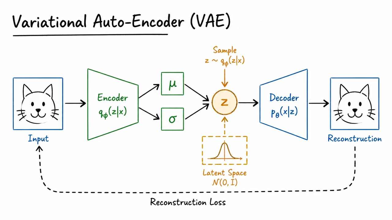
Before we can understand what a variational autoencoder is optimizing, we need to be precise about the problem it is trying to solve. A VAE is not merely an “autoencoder with noise.” It is a generative model: a model whose goal is to learn something about the probability distribution that produced the observed data.
Suppose we are given a dataset
where each observation . For images, might be the number of pixels; for audio, it might be waveform samples or spectrogram coefficients; for text embeddings, it might be the embedding dimension. The generative modeling problem is to learn a distribution that approximates the unknown data-generating distribution .
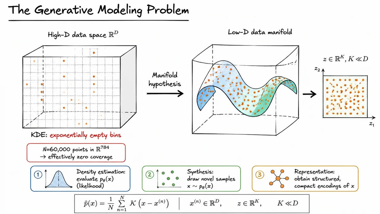
This goal has three closely related interpretations. First, we may want density estimation: given a new point , how likely is it under the model? That is, can we evaluate or approximate ? Second, we may want synthesis: can we draw new samples that look like plausible members of the dataset, but are not exact copies? Third, we may want representation learning: can the model discover compact, structured variables that explain meaningful factors of variation in the data?
These goals are connected, but they are not identical. A model may produce sharp-looking samples while assigning poor likelihoods, or it may achieve good likelihood while generating visually mediocre samples. VAEs are especially interesting because they try to tie these goals together through a probabilistic latent-variable framework: they define a likelihood, support sampling, and learn internal representations.
A first naive idea is to estimate the density directly from the observed data. For example, kernel density estimation places a small “bump” of probability mass around each training example:
In low dimensions, this can work surprisingly well. If the data points densely cover the relevant region of space, then nearby kernels overlap and form a smooth estimate of the distribution. But in high dimensions, this intuition breaks down catastrophically.
The reason is the curse of dimensionality. The volume of a ball of radius , or more generally the number of distinguishable regions in a -dimensional space, grows roughly exponentially with . For MNIST, a grayscale image lives in . Even images are vanishingly sparse in such a space. Almost every possible pixel vector is not a digit at all; it is visual noise. Worse, many distance-based intuitions fail: in very high dimensions, points tend to become nearly equidistant, making “nearest neighbors” and local smoothing much less reliable.
So the issue is not just that we need more data. The ambient space is overwhelmingly large, and the data occupies only a tiny, highly structured subset of it. A kernel density estimator spreads probability around observed examples in the ambient space, but most of that space is irrelevant. Unless the kernel bandwidth is extremely small, it assigns mass to unrealistic regions; if the bandwidth is extremely small, it assigns nearly zero density almost everywhere. Either way, the method fails to capture the actual structure of the data distribution.
This motivates the data manifold hypothesis. Although observations may be represented as vectors in a high-dimensional ambient space, the meaningful variation in the data often has much lower intrinsic dimension. For example, handwritten digits vary by stroke thickness, slant, rotation, identity, local style, and other factors. These factors are far fewer than 784 independent pixel degrees of freedom. Informally, the data may lie near a low-dimensional manifold embedded in the high-dimensional observation space.
This is where latent variables enter the story. Instead of modeling directly as an arbitrary point in the ambient space, we introduce a lower-dimensional variable
and imagine that observations are generated from these latent coordinates. The latent variable should capture the compact explanatory factors, while the model maps from latent space into data space. This does not mean the true data manifold is literally linear, smooth everywhere, or exactly -dimensional. Rather, it is a modeling assumption: useful data distributions often have enough low-dimensional structure that exploiting it is far better than treating all directions in equally.
The visual below condenses this motivation into a geometric picture. On the left, the high-dimensional ambient space is mostly empty: even many training examples provide negligible coverage when is large, which is why direct kernel-style density estimation becomes ineffective. On the right, the same data becomes much more intelligible when viewed as concentrated near a lower-dimensional manifold.
The key transition is from “estimate density everywhere in ” to “model how low-dimensional latent structure gives rise to high-dimensional observations.” That transition is the conceptual starting point for latent variable models, and it is exactly the path that will lead us to variational autoencoders.
The previous discussion framed generative modeling as a density-learning problem: we want a model that assigns high probability to realistic data and can also produce new samples. But high-dimensional observations—images, audio, text embeddings—rarely vary freely in all ambient dimensions. A handwritten digit image may have thousands of pixels, yet much of its variation can be described by a smaller set of factors: which digit it is, how thick the stroke is, whether it is tilted, how centered it is, and so on. Latent variable models make this intuition explicit.
The core assumption is that each observed data point is generated from an unobserved, lower-dimensional variable . We do not get to see in the dataset; it is a hidden explanation for the observation. Instead of modeling the distribution over directly, we define a two-step generative process:
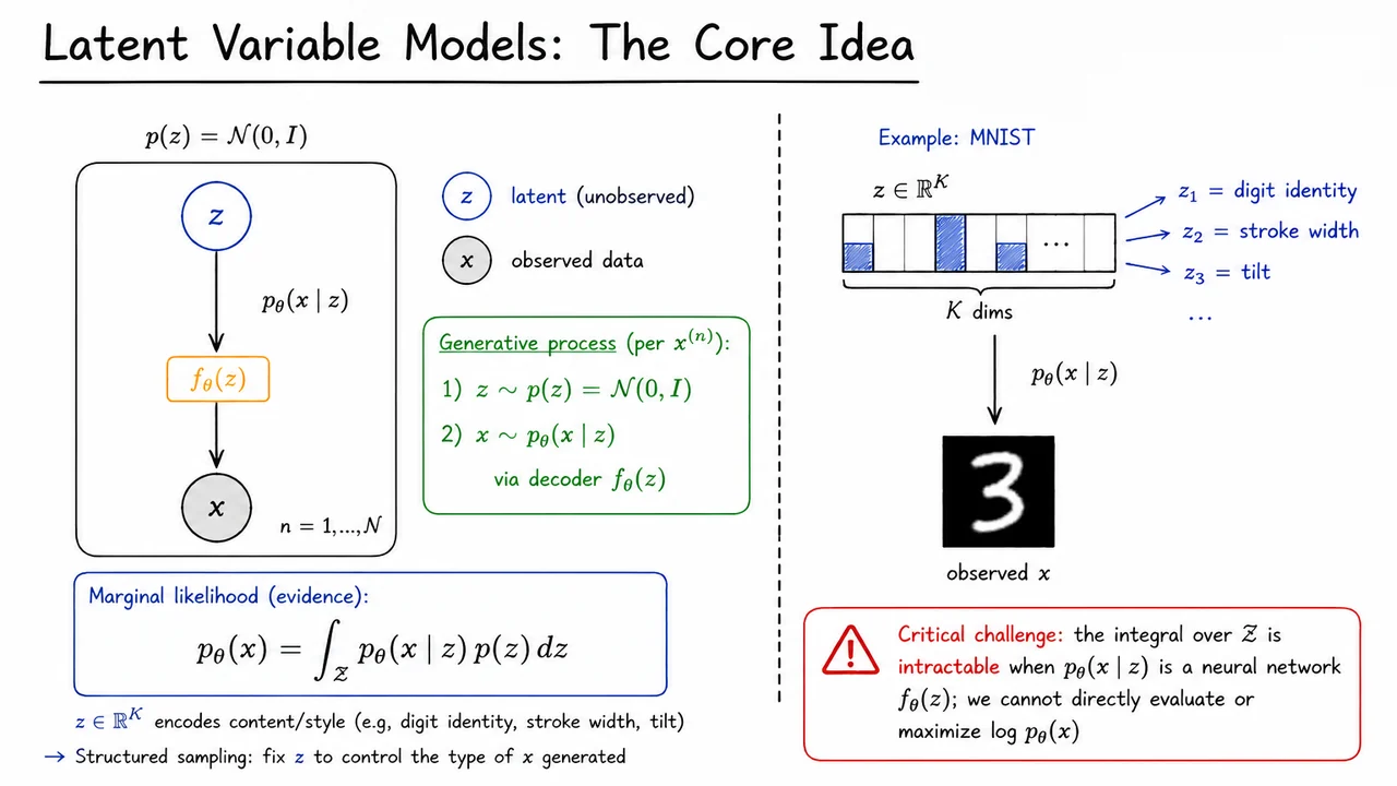
Here, is a simple prior over latent codes, usually chosen to be a standard Gaussian. The conditional distribution is the decoder or generative model: given a latent code, it describes a distribution over possible observations. In modern VAEs, this conditional distribution is parameterized by a neural network , which maps latent coordinates into the parameters of a likelihood over data space.
This setup separates two kinds of complexity. The prior is deliberately simple: sampling from is easy, and its geometry is well behaved. The decoder carries the burden of learning how simple latent variation becomes rich observed structure. For example, in an idealized MNIST model, nearby values of might correspond to visually similar digits, while different directions in latent space could control properties such as digit identity, stroke width, or tilt.
The probability assigned to an observation is obtained by considering all possible latent explanations that could have generated it. This gives the marginal likelihood, also called the evidence:
This integral is the mathematical heart of latent variable modeling. It says: to evaluate how likely is, average the likelihood over every possible latent code , weighted by how plausible that code was under the prior. A particular might reconstruct very well, but if that lies in an extremely unlikely region of the prior, its contribution is limited. Conversely, common latent codes contribute more, but only if the decoder can plausibly produce from them.
This is why latent variable models are so appealing. They offer a structured way to generate data:
They also offer a conceptual interpretation of representation learning: the model is encouraged to organize meaningful variation in data through the latent space. If the learned representation is smooth, moving through -space should produce coherent changes in generated samples rather than abrupt jumps.
But the same integral that makes the model principled also creates the central computational difficulty. When is parameterized by a neural network, the integral
usually has no closed form. The decoder can be highly nonlinear, and the latent space may have many dimensions. Direct numerical integration becomes infeasible, and naïve Monte Carlo estimates can be too noisy or inefficient for maximum likelihood training. Therefore, although the model defines formally, we cannot usually evaluate or maximize directly.
This is the key tension that motivates variational inference and, ultimately, the VAE objective. We have a clean generative story and a meaningful likelihood, but the marginalization over hidden causes is intractable. The rest of the VAE framework can be understood as a way to optimize a tractable surrogate for this inaccessible log-likelihood.
The visual below compactly summarizes this idea. The left side uses a graphical-model view: a latent variable is drawn from the prior, then an observed variable is generated through , repeated independently across data points. The shaded observed node emphasizes that is in the dataset, while remains hidden.
The right side grounds the abstraction in an MNIST-style example: a latent code can be thought of as controlling semantic or stylistic factors that the decoder turns into an image. The important warning is the intractable integral over : even though the sampling story is simple, evaluating the probability of a given observation requires summing over all latent explanations, which is precisely what we cannot do directly with a neural decoder.
Having introduced latent variable models, we now run into the first serious computational obstacle: the model is easy to write down, but hard to fit. The whole appeal was to define a simple prior , pass through a decoder, and obtain a flexible distribution over observations . But maximum likelihood training asks us to evaluate
and that integral is exactly where the trouble begins. For simple decoders, the integral and the posterior over latents may be analytically tractable. For neural network decoders, they usually are not.
The classical tool for latent variable models is Expectation-Maximization. EM alternates between inferring the latent posterior under the current parameters and then updating the parameters using expectations under that posterior. The E-step requires
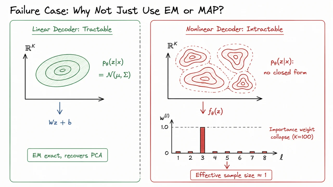
This equation is innocent-looking but deceptive. The denominator is the very marginal likelihood integral we were trying to avoid. In models with conjugacy or linear-Gaussian structure, the posterior has a known form and EM is elegant. But once the decoder becomes nonlinear, the posterior can become highly warped, multimodal, and unavailable in closed form.
A useful contrast is probabilistic PCA. Suppose
Because everything is linear and Gaussian, the posterior is also Gaussian. EM can compute its mean and covariance exactly. The latent space remains geometrically well-behaved: observing carves out an elliptical Gaussian belief over possible 's.
Now replace the linear map with a neural network :
The prior is still simple, and the observation noise may still be Gaussian, but the posterior is no longer Gaussian. The inverse image of a given observation under may contain many disconnected regions. Different latent codes can decode to similar observations. The posterior may have sharp ridges, separated modes, and strong nonlinear dependencies between latent dimensions. In other words, the generative direction may be easy to evaluate, while the inference direction is hard.
One tempting fallback is MAP inference: instead of representing the whole posterior, choose the most likely latent point,
This can be useful in some settings, but it is not a satisfactory replacement for posterior inference. A point estimate throws away uncertainty. If the posterior has several plausible modes, MAP picks one and ignores the rest. It also introduces an inner optimization problem for every datapoint, which is expensive during training. Worse, if we need gradients through that optimization procedure, the computation becomes cumbersome and brittle, especially when latent variables are discrete or when the optimization landscape is poorly conditioned.
Another seemingly generic solution is Monte Carlo EM. We might sample latent candidates from the prior,
and weight them according to how well they explain :
This is importance sampling with the prior as the proposal distribution. The problem is that the prior is usually a terrible proposal for the posterior. In high dimensions, most samples from land in regions that explain a specific extremely poorly. A tiny number of samples may receive almost all the probability mass, while the rest contribute essentially nothing.
This phenomenon is often called importance weight collapse. As the latent dimension grows, the effective number of useful samples can collapse toward one:
The phrase “effective sample size” is important: even if we draw thousands of samples, the estimator may behave as though it had only one meaningful sample. This creates exponentially high variance estimates of the E-step quantities and makes naive Monte Carlo learning impractical for expressive latent-variable models.
So the failure is not that EM, MAP, or Monte Carlo are conceptually wrong. Each is reasonable under the right assumptions. The failure is a mismatch between those assumptions and neural generative models:
The visual below compresses this comparison into the key geometric intuition. In the linear-Gaussian case, posterior inference is clean: the posterior over is a single Gaussian-shaped region, and EM can proceed exactly. In the nonlinear case, the posterior becomes irregular and multimodal, so the E-step no longer has a closed-form solution.
The weight-collapse sketch at the bottom emphasizes why simply sampling many 's from the prior does not rescue us. In high-dimensional latent spaces, almost all prior samples are irrelevant for a particular observation , and the importance weights concentrate on one lucky sample. This is the motivation for the next idea: instead of solving a separate hard inference problem from scratch for every datapoint, VAEs introduce amortized approximate inference—a learned encoder that predicts an approximate posterior directly.
The failure of direct EM or per-example MAP inference points us toward a different compromise: instead of solving a fresh optimization problem for every datapoint, we will learn a function that performs inference. This is the central move in a variational autoencoder. A VAE is not just “an autoencoder with noise”; it is a probabilistic latent-variable model equipped with a trainable approximation to the posterior.
The generative story begins with a latent variable , typically chosen to live in a relatively low-dimensional continuous space:
This distribution is called the prior. It says what kinds of latent codes are plausible before seeing any data. The standard Gaussian prior is not chosen because we believe the true hidden factors of images, text, or molecules are literally independent standard normal variables. Rather, it is chosen because it gives us a simple, smooth, sampleable reference distribution. Later, when we generate new data, we will sample and decode it into an observation.
The second ingredient is the decoder, also called the generative model or likelihood model. It specifies how an observed datapoint is produced from a latent code :
In a neural VAE, this conditional distribution is parameterized by a neural network . The network does not directly output “the reconstruction” in a purely deterministic sense; rather, it outputs the parameters of a probability distribution over possible observations. For continuous data, a common choice is an isotropic Gaussian likelihood,
where is the mean of the conditional distribution. For binary data, such as binarized MNIST pixels, a common choice is a Bernoulli likelihood,
Together, the prior and decoder define the actual generative model:
This joint distribution is the model’s claim about how data and latent variables co-occur. If we could compute the posterior exactly,
then inference would be straightforward: given an observed , infer which latent codes plausibly generated it. But the denominator,
is generally intractable for a nonlinear neural decoder. This is the same obstacle we encountered when trying to use exact EM: the posterior is the object we need, but it is not available in closed form.
The VAE introduces a third distribution to address this: the encoder, or approximate posterior,
Here another neural network, often denoted , maps an input datapoint to the parameters of a Gaussian distribution over latent codes:
This is an approximation to , not part of the generative model itself. The generative model is still . The encoder is an inference mechanism: it gives us a tractable distribution from which we can sample latent codes likely to explain .
The key innovation is amortized inference. In classical variational inference, we might introduce separate variational parameters for each datapoint, for example with its own . That would mean every new datapoint requires its own inference optimization. VAEs instead use a single shared network for all datapoints:
The cost of inference is therefore amortized over the dataset. We pay once to learn , and then inference for a new is just a forward pass. This is why VAEs scale well to large datasets and why they look architecturally like autoencoders: data goes through an encoder into a latent representation, then through a decoder back into data space. But probabilistically, the encoder and decoder play asymmetric roles.
There is also an important modeling assumption hidden in the standard encoder form. By choosing
we assume the approximate posterior is Gaussian with diagonal covariance. This makes sampling and KL-divergence computations convenient, but it can be restrictive. The true posterior may be multimodal, skewed, or highly correlated across latent dimensions. Much of the behavior of VAEs—including some failure modes we will discuss later—comes from the tension between a flexible neural decoder and a relatively simple approximate posterior family.
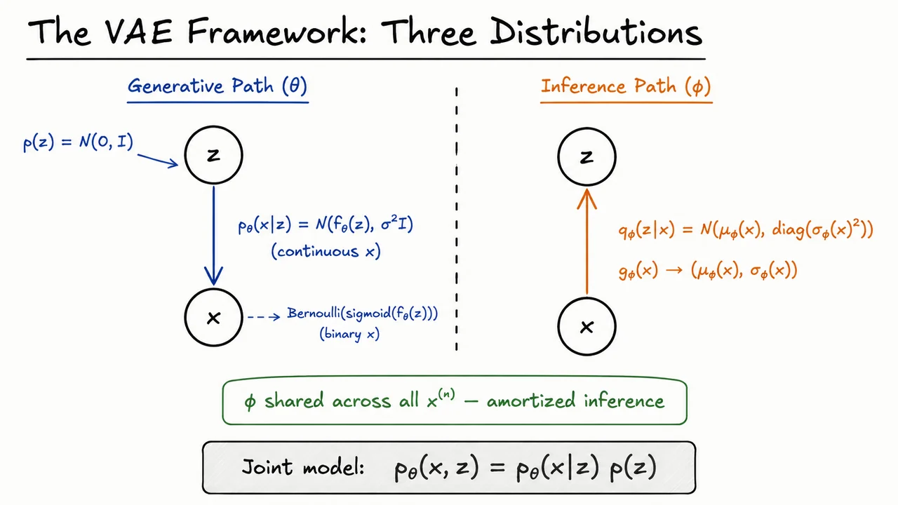
The three distributions therefore have distinct responsibilities:
The visual below consolidates this separation by showing two complementary paths. The generative path starts from and moves downward through to produce . The inference path goes in the opposite direction: given , the encoder produces a distribution over plausible latent codes.
The most important detail to keep in mind is that the right-hand path is not a separate model of the data. It is a learned approximation used to make training and inference tractable. The shared parameter vector is what makes the inference procedure amortized: instead of optimizing a new posterior approximation for every , the VAE learns one encoder network that serves the entire dataset.
Now that we have separated the VAE into its three distributions—the prior , the decoder , and the encoder-like approximation —we can ask the most basic statistical question: what objective should train the generative model? If the decoder is supposed to define a probability model over observations, then the natural answer is maximum likelihood. We want parameters that assign high probability to the observed dataset:
This is the same principle used in ordinary probabilistic modeling: choose the model under which the data would have been most likely. The complication is that in a latent-variable model, is not given directly. It is the probability of observing after averaging over all possible latent explanations .
For a single datapoint, the marginal likelihood, also called the evidence, is
so the log-evidence is
Conceptually, this integral says: sample a latent code from the prior, decode it into a distribution over , and average the probability assigned to the observed across all possible latent codes. If many plausible latent codes explain , the evidence should be high. If almost no latent code decodes near , the evidence should be low.
The problem is that this integral is almost never analytically tractable for a neural decoder. In a simple linear-Gaussian latent-variable model, the integral may have a closed form. But in a VAE, is parameterized by a deep network . The latent space is typically continuous, often , and the integrand can be nonzero over an enormous region. We are therefore trying to integrate a nonlinear neural-network-shaped function over a high-dimensional space:
There is no general symbolic simplification available.
A first instinct is to use Monte Carlo sampling from the prior. Draw
approximate the expectation, and then take the logarithm:
This looks reasonable, and for very large it is a consistent estimator. But as a training objective, it has two serious issues. First, prior samples are usually a terrible way to find the latent codes that explain a specific datapoint . In high dimensions, most will decode to samples unrelated to , so the average can be dominated by rare lucky samples. This leads to high variance.
Second, and more fundamentally, the log of a Monte Carlo average is a biased estimator of the log-evidence. The logarithm is concave, so Jensen’s inequality gives
The inequality is strict unless the random quantity inside the log is essentially constant. Equivalently, in the single-sample case,
This is the key obstruction: moving the logarithm outside or inside an expectation changes the objective. The log-evidence is what we want, but it contains an intractable integral. The expectation of the log-likelihood is tractable by sampling, but it is generally a lower quantity and, by itself, is not the right maximum-likelihood objective.
This is where the VAE’s central idea begins to emerge. We need a surrogate objective that is:
That surrogate will be the Evidence Lower Bound, or ELBO, written schematically as
The additional parameter appears because we introduce an inference network , whose role is to propose latent codes likely to explain the observed datapoint. Instead of sampling blindly from the prior, the VAE learns where in latent space to look.
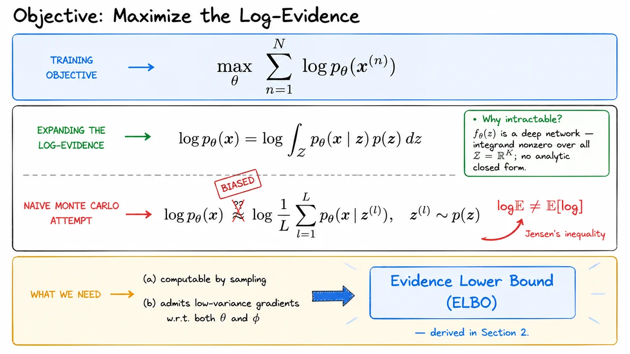
The visual below compresses this motivation into three layers: the maximum-likelihood goal, the intractable log-evidence integral, and the failed naive Monte Carlo shortcut. The red warning around Jensen’s inequality highlights the precise mathematical reason we cannot simply replace the integral with a sampled average inside a logarithm and proceed as if nothing changed.
The bottom layer then points to the resolution: rather than estimating the log-evidence directly, we construct a computable lower bound with good gradient behavior. The next step is to derive that bound carefully and see exactly why it is lower, when it becomes tight, and how it decomposes into the reconstruction and KL terms used in VAE training.
Having written the evidence as an integral over the latent variable, we now face the central obstacle of latent-variable maximum likelihood: the quantity we want,
is usually not computable in closed form. The integral sums over all possible latent explanations of the observation . For expressive neural decoders , this marginalization is precisely what makes the model powerful — and precisely what makes direct optimization difficult.
The key variational idea is to introduce an auxiliary distribution , which we will later implement as the encoder. At this point, however, is just a mathematical device: a distribution over latent variables conditioned on the observed datapoint. We use it to rewrite the intractable integral as an expectation under a distribution from which we can sample.
Starting from the evidence,
we multiply and divide by :
This is an exact algebraic identity, not an approximation. It is the same logic as importance sampling: instead of integrating directly with respect to the latent variable measure, we express the integral as an expectation under a chosen proposal distribution :
There is an important support condition hidden in this step. The ratio must be well-defined wherever contributes mass. Informally, must not assign zero probability to latent regions that the model considers possible explanations of . Otherwise, the importance-weighted expression can become undefined or miss parts of the integral entirely.
Now comes the only inequality in the derivation. Since is concave, Jensen’s inequality tells us that for a positive random variable ,
Here the random variable is
Applying Jensen’s inequality gives
or equivalently,
This lower bound is the evidence lower bound, or ELBO:
The name is literal: it is a lower bound on the log-evidence . For any valid choice of ,
This is the foundational move in VAEs. We replace an intractable objective with a tractable lower bound that can be estimated by sampling from the encoder.
The bound becomes tight exactly when Jensen’s inequality becomes equality. For a concave function like , equality occurs when the random variable inside the expectation is constant almost surely under . In this case, we need
Rearranging,
So the ELBO is tight when the variational distribution exactly matches the true posterior . This is also why the encoder is often described as an approximate posterior: it is trained to behave like the posterior distribution that would make the bound exact, but which is usually unavailable because it depends on the intractable evidence .
This derivation matters because it gives us a practical optimization target with a clear interpretation:
There is a subtle but important caveat: maximizing a lower bound is not automatically the same as maximizing the original objective. If the bound is loose, we may improve without significantly improving . The success of VAEs depends on making the variational family expressive enough, and the optimization stable enough, that this lower bound remains a useful surrogate for maximum likelihood.
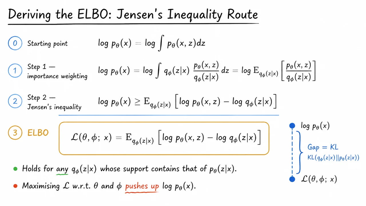
The visual below condenses the derivation into its three essential moves: start from the marginal likelihood, rewrite it as an expectation using , then apply Jensen’s inequality to move the logarithm inside the expectation. The boxed expression is the ELBO, the quantity we can optimize in place of the inaccessible log-evidence.
It also highlights the geometric meaning of the inequality: sits below , with a gap determined by how imperfect the variational posterior is. In the next section, we will decompose this same ELBO into the two terms that make VAEs operational: a reconstruction term and a KL regularization term.
Having obtained the ELBO through Jensen’s inequality, the next question is: what exactly are we optimizing? The expression
is already a valid lower bound on , but in this form it hides the two competing forces that make VAEs work. To understand the training objective operationally, we want to rewrite it in terms of the decoder likelihood and a penalty on the encoder distribution.
The key move is simply to expand the joint model. In a VAE, the generative story is assumed to factor as: first sample a latent variable from a prior , then sample the observation from a decoder likelihood . Therefore,
and taking logs gives
Substituting this into the ELBO gives
Because expectation is linear, we can separate the terms:
The first term has a direct modeling interpretation. We draw latent codes from the encoder distribution , then ask how much probability the decoder assigns back to the original observation . This is the reconstruction term:
It rewards latent representations that preserve information useful for explaining the input. If is a Bernoulli distribution, this often corresponds to a binary cross-entropy reconstruction objective; if it is a Gaussian with fixed variance, it becomes proportional to a negative squared-error loss. This is why VAEs often look, at implementation time, like autoencoders with a probabilistic reconstruction loss.
The second term is more subtle. Recall that the KL divergence is
Our ELBO contains the negative of this quantity:
So the ELBO decomposes into the now-famous form
This decomposition explains the central tension in VAE training. The reconstruction term wants to encode enough information about that the decoder can reconstruct it accurately. The KL term wants to stay close to the prior , usually a simple standard Gaussian such as . In other words, the encoder is not free to assign every datapoint an arbitrary isolated latent code; its codes must remain compatible with a shared latent space from which we can later sample.
This regularization is not merely aesthetic. Without it, the model could behave like an ordinary deterministic autoencoder: excellent reconstructions, but a latent space with holes, disconnected regions, and no reliable way to generate new samples by drawing . The KL penalty pushes the aggregate structure of the latent codes toward something smooth and sampleable. At the same time, if the KL pressure is too strong, the encoder may ignore , producing for every input. That failure mode is known as posterior collapse, and it causes the latent variable to carry little or no information.
A useful way to remember the objective is:
For the common Gaussian case, this tradeoff becomes especially convenient computationally. If
and
then the KL term has a closed-form expression. That means VAE training usually combines a Monte Carlo estimate of the reconstruction expectation with an analytic KL penalty, giving a stable and differentiable objective once we introduce the reparameterization trick.
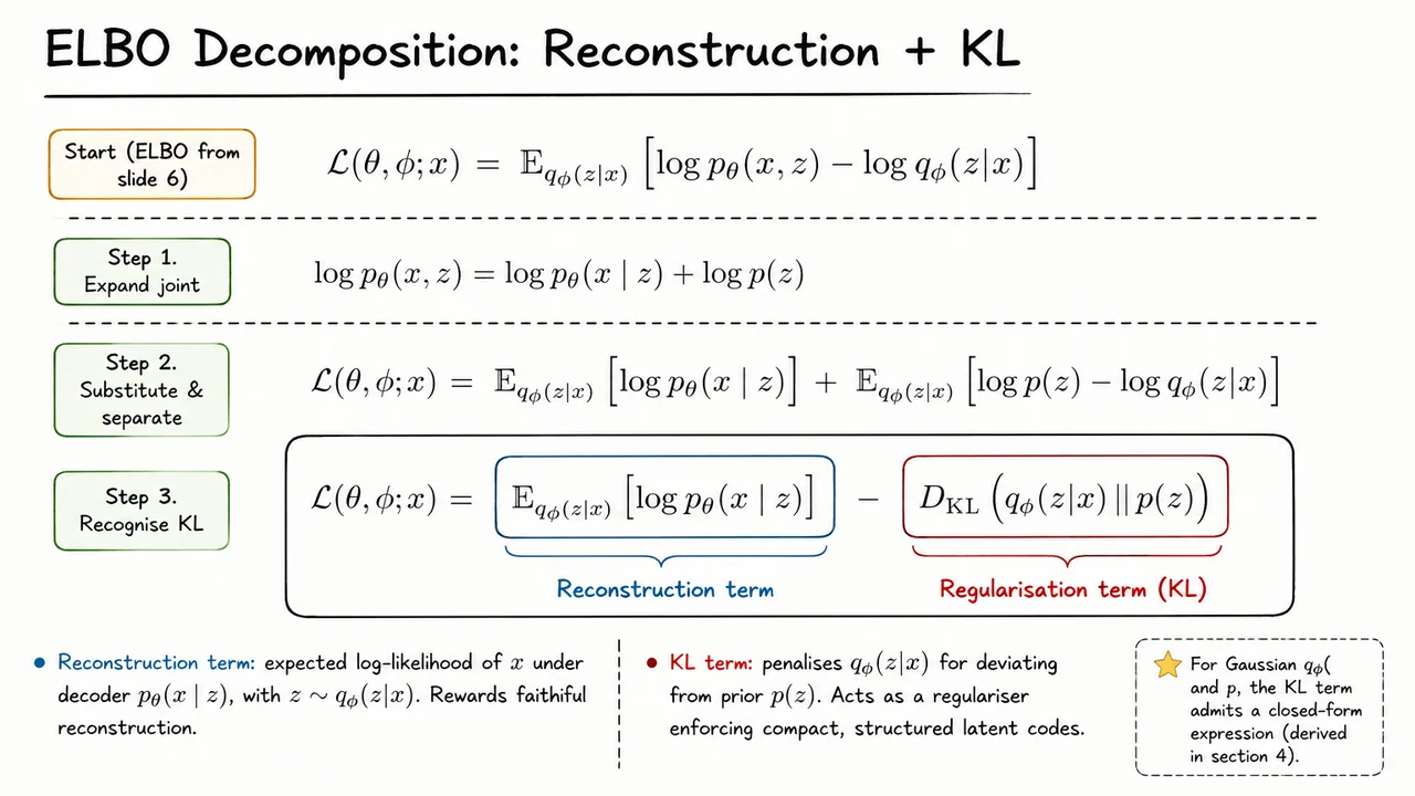
The visual below condenses this derivation into its algebraic skeleton: start from the Jensen-derived ELBO, expand the joint distribution using the generative factorization, separate the expectation, and recognize the second piece as a negative KL divergence. The color split emphasizes that the final objective is not one monolithic loss, but a sum of two interpretable forces with opposite pressures.
Read the final boxed equation as the practical training objective for a single datapoint : maximize expected decoder log-likelihood while minimizing deviation from the prior. This compact decomposition is the bridge between the abstract variational bound and the loss function we will soon implement in an actual VAE.
Having split the ELBO into a reconstruction term and a KL-to-prior regularizer, we can now ask a deeper question: what exactly did we lose when we replaced the true log-evidence by the ELBO? The answer is one of the most important identities in variational inference: the missing quantity is not mysterious approximation error, nor a loose heuristic penalty. It is exactly a KL divergence between the variational encoder and the true Bayesian posterior.
For a latent-variable model, the evidence is
and the true posterior over latents is
This posterior is the distribution we would ideally use for inference: after observing , it tells us which latent explanations are plausible. The difficulty is that depends on , the very integral we cannot usually compute. VAEs therefore introduce an encoder , a tractable approximation to this intractable posterior.
The central theorem says that, for a suitable variational distribution ,
Here the ELBO is
So the ELBO is not merely inspired by the evidence. It is the evidence minus a very specific nonnegative gap.
Because KL divergence is always nonnegative,
we immediately recover the lower-bound property:
This also explains the name Evidence Lower Bound. The ELBO sits below the log-evidence, and the vertical distance between them is precisely the mismatch between the approximate posterior and the true posterior .
The theorem also tells us exactly when the bound is tight. We have
if and only if
In words: the ELBO becomes the true log-evidence exactly when the encoder recovers the true posterior. There is no remaining variational gap. This is why the encoder is not just an auxiliary neural network used for amortized sampling; it is performing approximate Bayesian inference.
There is a subtle support assumption hiding here. For the KL
to be finite, should not place probability mass where the true posterior has zero mass. More formally, we usually require to be absolutely continuous with respect to . At the same time, if the variational family is too restrictive and cannot represent the true posterior’s important regions, the gap cannot close. This is one reason why posterior approximation quality depends not only on optimization, but also on the expressiveness of the encoder family.
The identity has an important optimization consequence. Suppose is fixed. Then is constant with respect to , so maximizing the ELBO over is exactly equivalent to minimizing
That is the variational inference interpretation of the VAE encoder: training by maximizing the ELBO pushes it toward the true posterior. When we also optimize , we are doing two things at once: learning a generative model that assigns high probability to the data, and learning an approximate inference model that explains each datapoint in latent space.
A useful way to remember the theorem is:
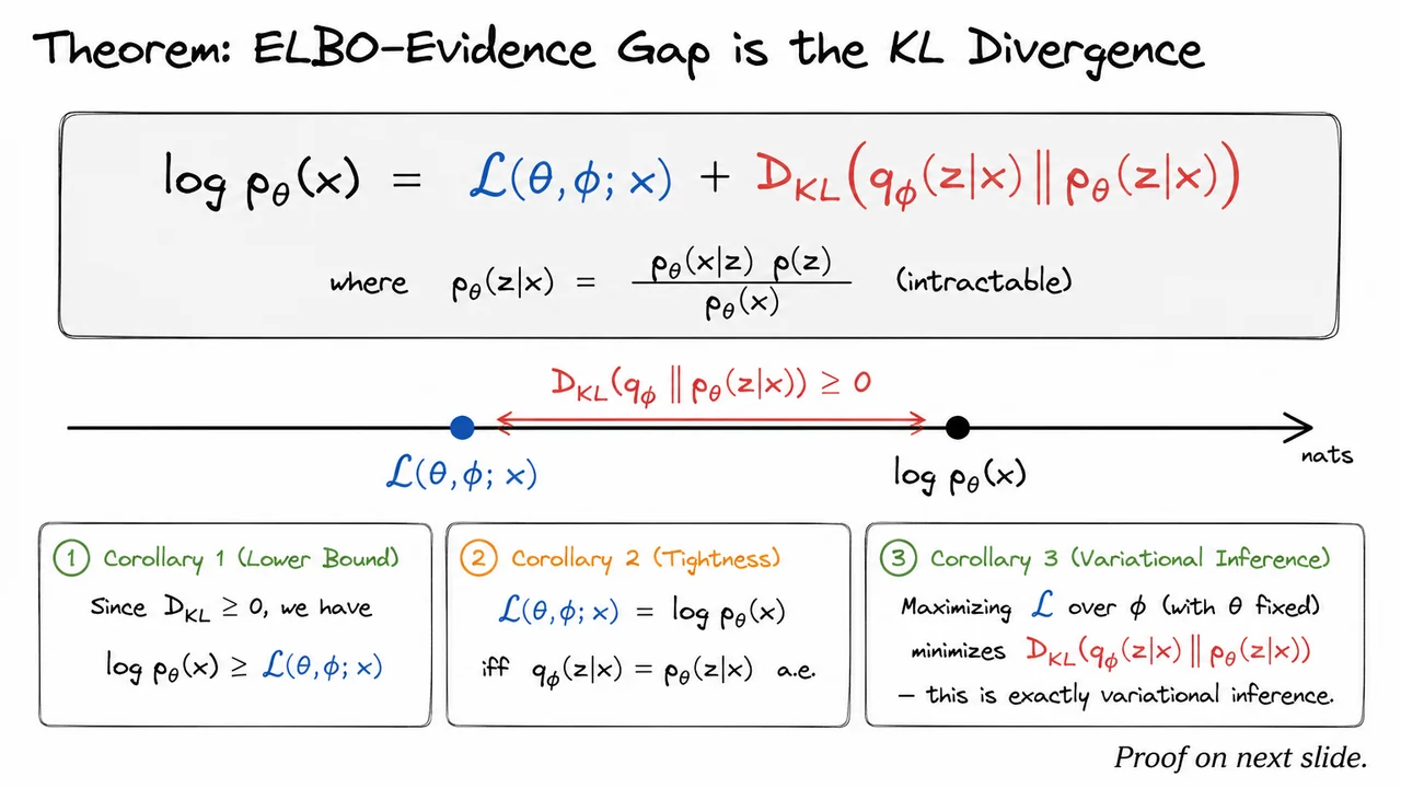
The visual below compresses this relationship into a geometric picture. The log-evidence is represented as a fixed point on a “nats” axis, while the ELBO lies to its left. The red interval between them is the posterior KL divergence. If the encoder improves, that interval shrinks; if matches , the two points coincide.
The three corollaries in the visual are therefore not separate facts, but direct consequences of the same decomposition: the ELBO is a lower bound because KL is nonnegative; it is tight exactly when the approximate and true posteriors agree; and maximizing it with respect to is variational inference. The next step is to prove the identity algebraically, showing how Bayes’ rule turns the apparently inaccessible evidence into the sum of an optimizable lower bound and an explicit posterior mismatch term.
Having stated that the gap between the log evidence and the ELBO is a KL divergence, we should now verify that this is not a heuristic slogan. It is an exact identity. The derivation is short, but it is worth reading carefully because it explains why variational inference works: we are not inventing an arbitrary surrogate objective; we are decomposing the true marginal log-likelihood into a tractable lower bound plus a nonnegative error term.
Fix one observed datapoint . The model defines a latent-variable joint distribution
and the true posterior is
The problem is that , the evidence, usually requires integrating out :
In a VAE, this integral is generally intractable because the decoder is represented by a neural network. So instead of working directly with the true posterior , we introduce an approximate posterior, or encoder distribution,
The key question is: how does optimizing an objective involving relate to maximizing the true log evidence ?
Start from the KL divergence between the variational posterior and the true posterior:
Now substitute Bayes’ rule into the true posterior term:
Taking logs gives
Therefore,
The subtle but crucial observation is that does not depend on . The expectation is over , while is fixed. So we can pull outside the expectation:
Equivalently,
The expectation inside the negative sign is precisely the evidence lower bound:
So the KL divergence becomes
Rearranging gives the central decomposition:
This is the whole proof. No approximation has been made. We used only the definition of KL divergence, Bayes’ theorem, and the fact that constants can be moved outside expectations.
The consequence is immediate. Since KL divergence is always nonnegative,
we have
That is why is called a lower bound on the log evidence. The bound is tight exactly when
which occurs when
almost everywhere under . In words: the ELBO equals the true log evidence when the encoder distribution exactly matches the model’s true posterior.
This identity also clarifies a common failure mode in variational modeling. Maximizing the ELBO improves a lower bound on , but it does so through the restricted family . If the encoder family is too limited, the KL gap may remain large even after optimization. The objective is still valid, but the approximation may be poor. Conversely, if is expressive enough and optimization succeeds, the ELBO can become a very accurate proxy for the true marginal likelihood.
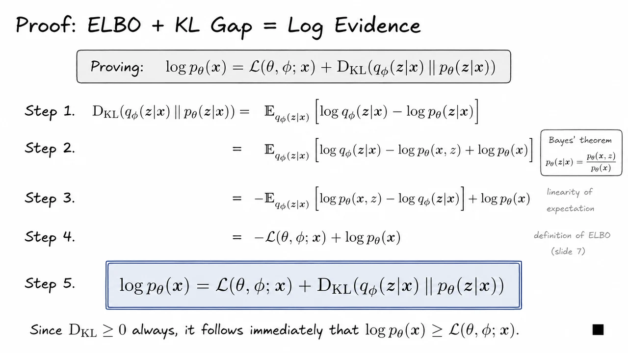
The visual below compresses the derivation into a chain of equalities: start with the KL divergence to the true posterior, replace the posterior using Bayes’ theorem, separate the constant , recognize the ELBO, and rearrange. The boxed final identity is not an additional assumption; it is simply the same expression written so that the evidence appears on the left.
It is useful to keep this picture in mind as we move forward. The ELBO is not merely “reconstruction plus regularization” yet—that interpretation will come after expanding the joint model. At this stage, the most important fact is structural: log evidence decomposes exactly into an optimizable lower bound plus a nonnegative posterior-approximation gap.
Having just seen that the ELBO differs from the true log evidence by a nonnegative KL gap, we can now reinterpret the bound in a more operational way. The ELBO is not merely an algebraic trick for lower-bounding ; it is the objective that tells a VAE how to trade off using latent information against staying compatible with the prior.
For a single datapoint , the VAE objective is
The first term is the reconstruction term. It asks: if the encoder distribution samples a latent code , how much probability does the decoder assign back to the original observation ? Maximizing this term encourages the latent representation to preserve information that the decoder needs. In an image VAE, this means encoding shape, pose, color, texture, or any features that help predict the input under the chosen likelihood model.
The second term is the regularization term, but that phrase can be slightly misleading if we think of it as a generic penalty. More precisely, it penalizes the encoder distribution for moving too far away from the prior , usually . This matters because generation will later sample , not . If the encoder learns latent codes that live in strange isolated regions far from the prior, then samples drawn from the prior may decode poorly. The KL term forces the aggregate geometry of the latent space to remain usable for generation.
We can unpack the KL penalty further using
Therefore,
This decomposition reveals two forces hidden inside the regularization term. The entropy term rewards the encoder for being uncertain, or spread out, rather than collapsing to a deterministic point code. Meanwhile, the expected negative log prior term penalizes codes that fall in regions where assigns low probability. For a standard Gaussian prior, this means the model is discouraged from placing latent mass far away from the origin.
So the ELBO is balancing two competing desires:
This tension is fundamental. If the KL penalty is too weak, the encoder may memorize examples using highly specialized latent codes, producing good reconstructions but a poorly organized latent space. If the KL penalty is too strong, the encoder may ignore and make , which can lead to posterior collapse: the decoder receives little useful information from , and the latent variables stop carrying semantic structure.
This is why the ELBO also has a natural rate–distortion interpretation. The KL term acts like a rate: it measures how many nats, or bits up to a constant conversion, are required to encode using a distribution different from the prior. The reconstruction error acts like a distortion: poor reconstructions correspond to high distortion, while high log-likelihood corresponds to low distortion. Maximizing the ELBO means finding a good operating point between compression cost and reconstruction fidelity.
The connection to physics and variational inference comes from writing the training problem as minimization of the negative ELBO:
This quantity is often called the variational free energy or negative evidence lower bound. Since we previously established
minimizing free energy simultaneously pushes the ELBO upward and tries to reduce the gap between the approximate posterior and the true posterior . The bound becomes tight exactly when
assuming the variational family is expressive enough to represent the true posterior.
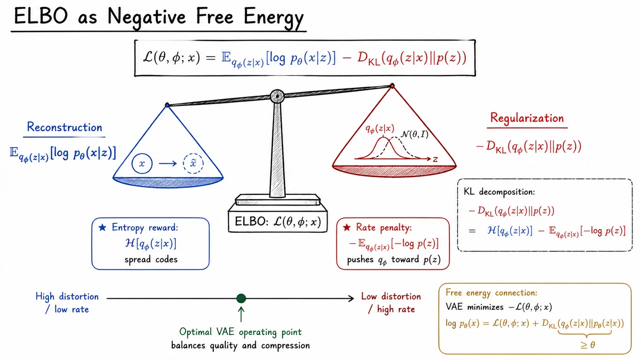
The visual below condenses this interpretation into a balance: reconstruction pulls the objective toward faithful recovery of , while KL regularization pulls the encoder distribution back toward the prior. The scale metaphor is useful because neither side is “bad”; a good VAE needs both. Reconstruction gives the latent variable meaning, while the KL term gives the latent space global structure.
It also highlights the rate–distortion view: moving toward lower distortion usually requires spending more rate, while enforcing a very low rate often sacrifices detail. Much of practical VAE design—choosing decoder likelihoods, KL schedules, -VAE objectives, or more expressive priors—is about controlling exactly where this operating point lies.
Having seen the ELBO as a negative free energy, it is worth pausing on a case where nothing is hidden behind approximation. In most VAE settings, the posterior is intractable, which is exactly why we introduce a variational distribution . But in a one-dimensional linear-Gaussian model, the posterior, marginal likelihood, KL terms, and ELBO can all be written down exactly. That makes it a useful sanity check: if our interpretation of the ELBO is right, then optimizing it over a sufficiently expressive variational family should recover the true posterior and make the ELBO equal to the evidence.
Consider the toy generative model
Here the latent variable is drawn from a standard normal prior, and the observation is a noisy version of with small Gaussian noise variance . Because both the prior and likelihood are Gaussian, the marginal distribution of is also Gaussian:
so the log evidence is available in closed form:
The true posterior is also Gaussian. Combining the prior precision with the likelihood precision , the posterior variance is
and the posterior mean is the precision-weighted estimate
Thus
This already contains an important intuition. The observation pulls the posterior mean toward , but not all the way: the prior still shrinks the estimate toward zero. Since the observation noise is small, the posterior variance is much smaller than the prior variance. For , we get
Now suppose our variational family is
This family is expressive enough to contain the true posterior exactly, because the true posterior is also a one-dimensional Gaussian. The ELBO is
In this Gaussian case, both terms can be evaluated analytically. The expected reconstruction term is
because under ,
The KL regularizer against the standard normal prior is
So the ELBO is a deterministic function of only two variational parameters, and . There is no Monte Carlo noise, no neural network approximation, and no optimization mystery. We can inspect the entire objective surface directly.
The key identity from the previous section was
Because the evidence does not depend on , maximizing the ELBO over is equivalent to minimizing
In this toy example, the minimum possible KL gap is exactly zero, since the variational family contains the true posterior. Therefore the global maximizer is
or equivalently,
At that point,
and the ELBO becomes tight:
This is the tightness corollary in its cleanest possible form.
It is useful to compare three operating points for :
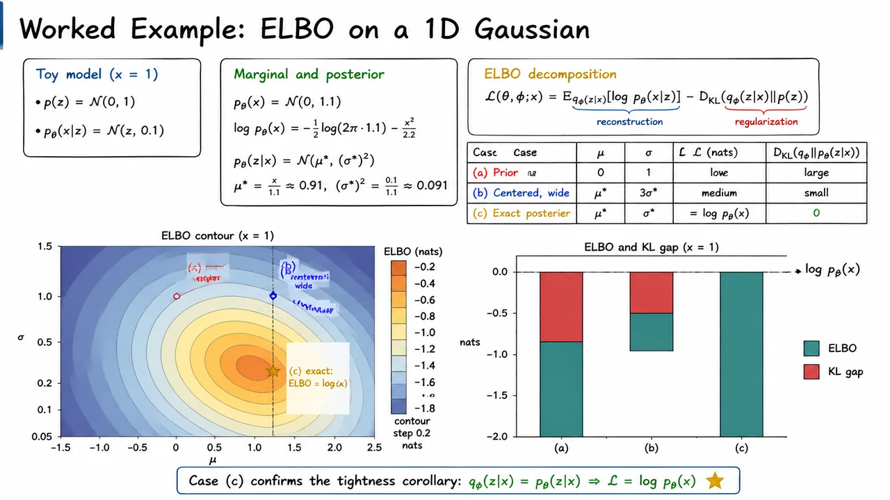
The visual below consolidates these facts in two complementary ways. The contour plot treats the ELBO as a surface over : the maximum occurs exactly at the true posterior parameters, not merely near them. The prior-like approximation sits far away from the optimum, while the centered-but-wide approximation lands on the correct mean but remains suboptimal because its uncertainty is wrong.
The companion bar chart emphasizes the decomposition
For each candidate , the ELBO plus the KL gap reaches the same evidence level. In the exact posterior case, the red “gap” disappears entirely, making the lower bound not just a bound, but the true log marginal likelihood.
The one-dimensional Gaussian example makes the ELBO feel almost deceptively friendly: the KL term can be written down, the expectation can sometimes be evaluated or estimated, and the whole objective looks like something we should be able to optimize with ordinary backpropagation. But the moment we replace that toy setup with a neural encoder and decoder, a subtle obstruction appears. The problem is not that the ELBO is undefined, nor that Monte Carlo estimation is impossible. The problem is that the Monte Carlo samples themselves sit in the middle of the computation graph.
Recall that for a single datapoint , the VAE objective is
When we differentiate with respect to the encoder parameters , the gradient decomposes as
The KL term is usually not the source of trouble in the standard VAE. If is a diagonal Gaussian,
and the prior is , then the KL divergence has a closed form. It is just a differentiable expression involving and . Autodiff can handle this directly.
The reconstruction term is different because the distribution inside the expectation depends on :
Here controls where we sample from. Changing changes the density , which changes the regions of latent space that contribute to the expectation. This is not the same as differentiating an ordinary deterministic function. The parameter affects the objective through the sampling distribution itself.
A natural first attempt is to use Monte Carlo sampling. Draw
and approximate the reconstruction expectation by
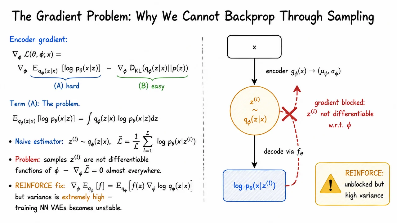
This gives an unbiased estimate of the expectation. For optimizing , it is fine: once is sampled, the decoder likelihood is an ordinary differentiable function of . But for optimizing , naive backpropagation runs into a wall. The sampled value is not represented as a differentiable deterministic function of . In the computation graph, the operation “sample from ” behaves like a stochastic node, not like a smooth layer.
This is the key failure mode of naive Monte Carlo:
does not correctly estimate
If we treat the sampled values as fixed constants after sampling, then the reconstruction term has no differentiable path back to . Informally, the gradient is blocked at the sampling operation. More precisely, the particular sampled numerical value may change if we rerun the sampler with a different , but that dependence is not available to standard backpropagation as a local derivative through the realized sample.
There is a general-purpose workaround called the score-function estimator, often known in this context as REINFORCE. It uses the identity
This identity is valid under mild regularity assumptions and does not require differentiating through the sampled value . Instead, it differentiates the log-density of the sampling distribution. That is powerful: it works even for discrete random variables, where ordinary pathwise derivatives are unavailable.
But for VAEs with neural decoders, this estimator is usually too noisy to be practical without substantial variance reduction. The scalar reward-like term can vary dramatically across samples, especially early in training. Multiplying it by often produces gradients with very high variance. In principle the estimator is unbiased; in practice, its updates can be so unstable that learning becomes slow, erratic, or ineffective.
So the issue is not merely “sampling is random.” The deeper issue is that we need a low-variance differentiable estimator of how the reconstruction objective changes when the encoder distribution changes. Naive Monte Carlo gives samples but no usable pathwise gradient. REINFORCE gives a gradient but often with prohibitive variance. This tension is exactly what motivates the reparameterization trick.
The visual below compresses this obstruction into a computation graph. The forward pass is straightforward: is encoded into parameters of , a latent sample is drawn, and the decoder evaluates . The backward pass is where the asymmetry appears: gradients flow cleanly through the decoder, but the attempted gradient path back through the stochastic sampling node is blocked.
The small REINFORCE annotation is the important caveat. There is a mathematical gradient estimator that avoids differentiating through the sample, but it pays for that generality with high variance. The next step is to replace the problematic sampling operation with an equivalent differentiable construction—one that preserves the same distribution over , while allowing backpropagation to reach .
The obstruction we just ran into was not that the encoder distribution is mysterious, nor that Gaussian sampling is impossible to differentiate in some philosophical sense. The issue is more specific: if we treat the operation “draw ” as an opaque stochastic node, then the sampled value changes with only through the distribution from which it was drawn. Standard backpropagation expects deterministic computational paths; it does not know how to assign a pathwise derivative through the act of sampling itself.
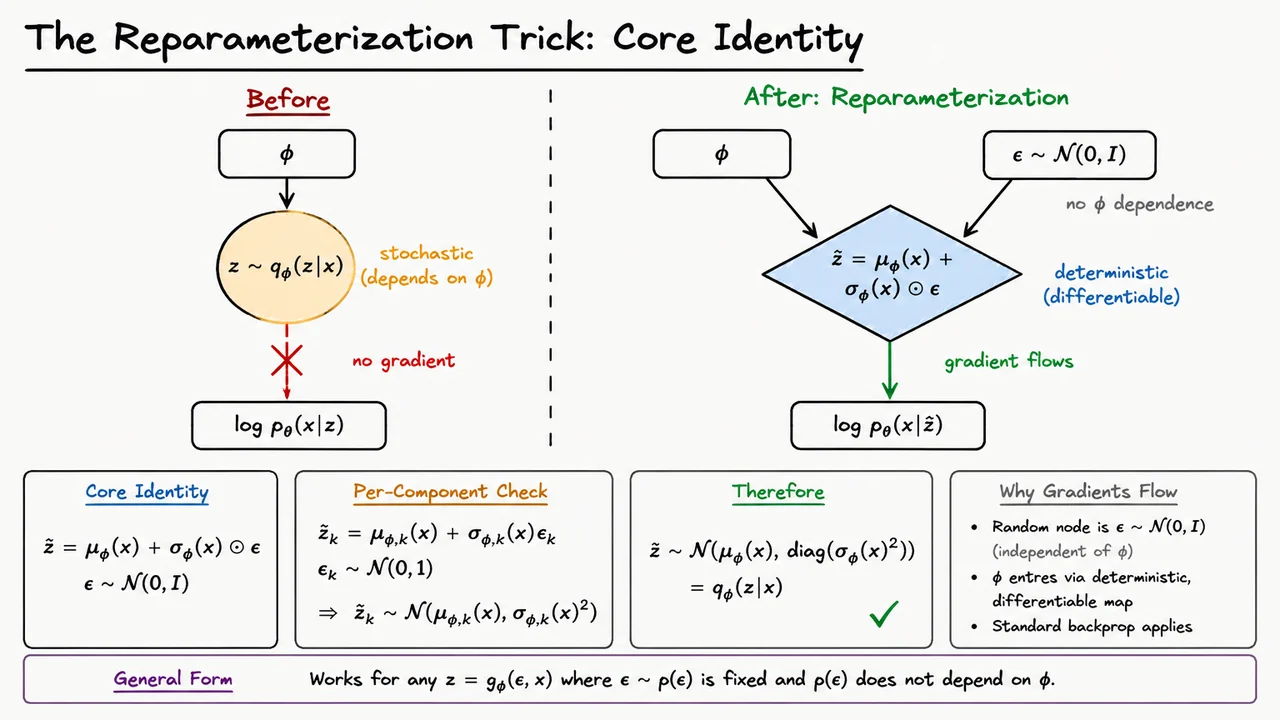
The reparameterization trick resolves this by changing how we generate the same random variable. Instead of sampling directly from a -dependent Gaussian, we sample from a fixed, parameter-free source of randomness and then transform that noise deterministically using the encoder outputs. For the diagonal Gaussian encoder used in the standard VAE,
we write a sample as
This is the core identity. The randomness now lives entirely in , whose distribution does not depend on . The encoder parameters only determine the deterministic map that takes to .
It is worth verifying that this has not changed the distribution being sampled. Componentwise,
An affine transformation of a standard normal random variable is normal, with shifted mean and rescaled variance:
Since the are independent under , the resulting vector has diagonal covariance:
So the reparameterized sample is distributionally identical to a direct sample from the encoder. The trick is not an approximation to the Gaussian; it is an exact change of representation.
The important shift is computational. Before reparameterization, we had a sample , and the dependence of on was hidden inside the sampling operation. After reparameterization, we have
where is treated as an external random input. For a fixed draw of , the map from to is just an ordinary differentiable computation graph. Gradients can flow through , through , and then through the decoder likelihood term .
This is why the reparameterization trick is sometimes called a pathwise gradient estimator. Instead of asking how the probability density changes with , we ask how the sampled point moves in latent space when changes while holding the underlying noise fixed. Intuitively, chooses a location in “standard normal coordinates,” and the encoder stretches and shifts that location into the latent space used by the decoder.
For example, if increasing one encoder parameter increases , then every sampled shifts upward by the corresponding amount. If increasing another parameter increases , then samples with positive move upward and samples with negative move downward. These are ordinary derivatives:
Backpropagation can now see exactly how changing the encoder changes the latent sample and, through the decoder, changes the reconstruction term in the ELBO.
There are a few assumptions hiding here. First, we need a distribution that can be expressed as a deterministic transformation of parameter-free noise. This is easy for location-scale families such as Gaussians, where samples can be written as “mean plus scale times noise.” Second, the transformation should be differentiable with respect to the parameters we want to optimize. Third, the base noise distribution must not depend on ; otherwise the original problem reappears inside the supposedly fixed randomness.
In its most general form, the idea is
where is fixed and is differentiable. The diagonal Gaussian VAE is the canonical example, but the principle extends beyond it whenever such a transformation is available. When it is not available—for example, for many discrete latent variables—we need different gradient estimators or relaxations, and those usually come with higher variance or bias.
The visual below compresses this logic into two computation graphs. The left side represents the problematic formulation: determines a distribution, a stochastic sample is drawn, and the gradient path is interrupted at that sampling node. The right side rewrites the same sample as a deterministic function of encoder outputs and independent noise. The stochasticity has not disappeared; it has simply been moved to a place where it no longer carries -dependence.
The key message to carry forward is that reparameterization does not make the VAE deterministic. Each forward pass can still use a fresh , so the latent code remains random. What changes is that, conditional on that noise draw, the ELBO becomes an ordinary differentiable objective with respect to . That is the bridge from stochastic latent-variable learning to standard neural-network optimization.
Having rewritten sampling as , the next question is not merely whether this is a convenient implementation trick. The real question is whether it gives us the right gradient. If we replace a draw from with a deterministic transformation of noise, are we still estimating
without bias?
This matters because the VAE objective contains expectations over latent variables sampled from the encoder distribution. For a single datapoint , the reconstruction-related part of the ELBO often has the form
where, for example, may be . The encoder parameters affect this expectation indirectly: changing changes the distribution over . Naively sampling creates a problem for backpropagation because the sampling operation itself is not a deterministic differentiable map of .
The reparameterization trick resolves this by expressing the random variable as
Now all randomness lives in , whose distribution does not depend on . The dependence on has been moved into a deterministic function:
So instead of differentiating through the act of sampling from , we differentiate through the deterministic path
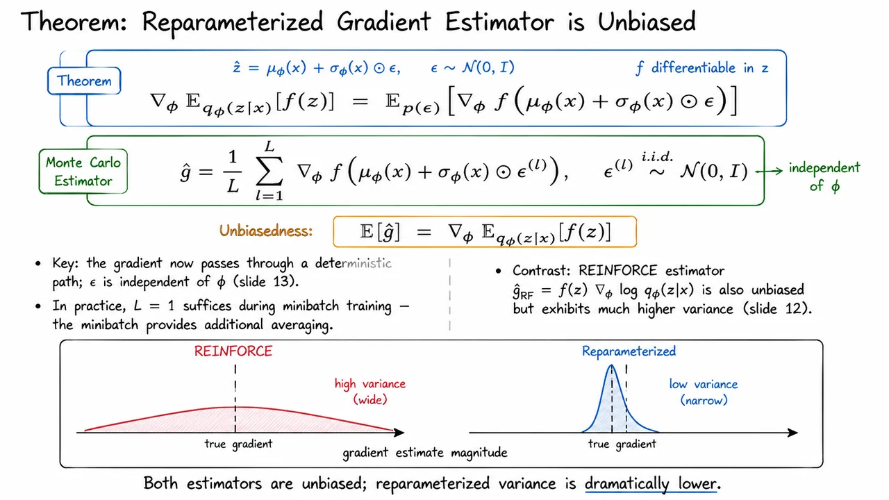
The theorem states that, under the usual smoothness and integrability assumptions that allow us to interchange differentiation and expectation,
This is the central identity. The left side is the gradient we actually want: the derivative of an expectation under the encoder distribution. The right side is something we can estimate by ordinary backpropagation after sampling . Importantly, the expectation is now over , a fixed distribution independent of .
Given independent samples , the Monte Carlo estimator is
Because each term inside the average is an unbiased draw from the expectation on the right-hand side of the theorem, linearity of expectation gives
So the estimator is unbiased: averaging over repeated draws of , it recovers the exact gradient of the expected objective.
There are a few assumptions hiding inside this clean statement. First, must be differentiable with respect to , and the transformation from to must also be differentiable. This is why the standard Gaussian VAE encoder, parameterized by and , is so convenient. Second, the support of the distribution should not change in a pathological way as changes; otherwise, differentiating under the integral can become delicate. Third, the estimator is unbiased for the gradient of the reparameterized expectation, but finite-sample estimates still have variance. Unbiased does not mean noiseless.
The reason this estimator is so effective is not only that it is unbiased, but that it tends to have low variance. Compare it to the score-function or REINFORCE estimator:
REINFORCE is also unbiased and applies more generally, including to discrete random variables. But it usually has much higher variance because it does not exploit the local derivative . It treats more like a black-box reward. The reparameterized estimator, by contrast, uses the geometry of : gradients flow through the sampled latent value back into and .
This explains a practical fact about VAEs: we often use latent sample per datapoint during training. At first this may seem surprisingly crude, but minibatch stochastic optimization already averages gradients across many datapoints. The total gradient noise comes from both minibatch sampling and latent-variable sampling; in practice, the low variance of the pathwise gradient makes a single latent draw per example sufficient for stable learning.
The visual below condenses this theorem into two linked ideas. The top part emphasizes the algebraic identity: a gradient of an expectation under can be rewritten as an expectation over fixed noise , with gradients traveling through the deterministic map . The key annotation is that is independent of , which is precisely what makes ordinary backpropagation valid.
The bottom part gives the statistical intuition. Both REINFORCE and the reparameterized estimator are centered on the true gradient, so both are unbiased. But the REINFORCE distribution is much wider, representing high-variance gradient estimates, while the reparameterized estimator concentrates much more tightly around the true value. That difference in variance is what turns the theorem from a formal identity into a practical training method for VAEs.
Now that we know the reparameterized gradient estimator is unbiased, it is worth slowing down and asking why the identity is true. The key point is not mysterious: we are simply rewriting a -dependent distribution as a deterministic transformation of noise drawn from a fixed distribution. Once the randomness no longer depends on , differentiation becomes an ordinary backpropagation problem through a deterministic computation graph.
Start with the quantity we care about. For a fixed datapoint , suppose the encoder distribution is a diagonal Gaussian,
and suppose is some downstream scalar objective term, such as a decoder log-likelihood contribution. We want the gradient
The difficulty is that the distribution inside the expectation depends on . If we sample , the sample itself changes as the encoder parameters change, but this dependence is not explicit in the notation. Naively differentiating through a random draw is not well-defined in the usual computational graph sense.
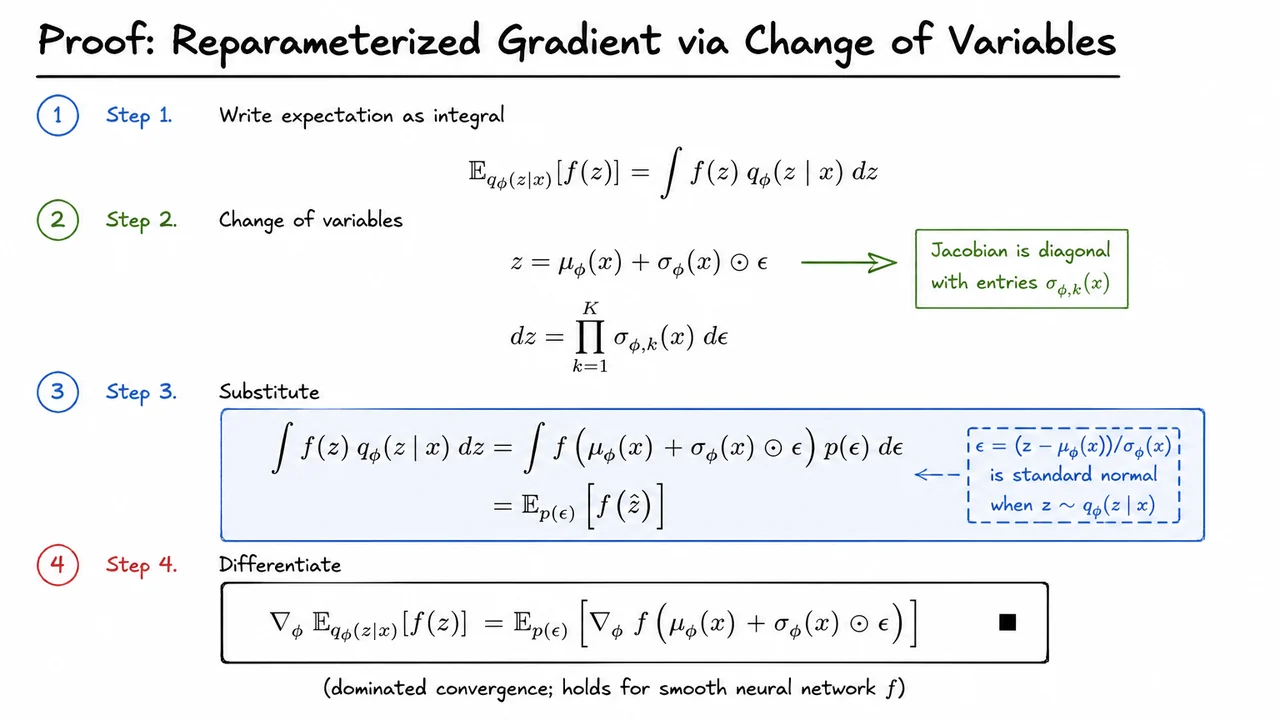
Writing the expectation as an integral makes the dependency explicit:
Here, appears in the density . A score-function estimator would differentiate the density directly, producing terms involving . That approach is general, but often high-variance. The reparameterization trick instead asks whether we can move the -dependence out of the density and into the argument of .
For a diagonal Gaussian, we can. Let
and define
This deterministic transformation maps standard normal noise into a sample from . Componentwise,
Assuming , this map is invertible in each coordinate:
The Jacobian is diagonal, with entries , so the volume element transforms as
This is the whole mathematical engine of the proof. Under the change of variables , the original density-weighted measure becomes
Therefore,
Equivalently,
Notice what changed. The distribution is now fixed: it does not depend on . All dependence on has moved into the deterministic map
That is why backpropagation becomes possible. We are no longer differentiating “through sampling” from a moving distribution; we are differentiating through a deterministic function of fixed external noise.
Under the usual regularity assumptions—smooth enough , differentiable encoder outputs, and an integrable dominating function allowing us to exchange differentiation and integration—we can pass the gradient through the expectation:
Combining the equality of expectations with this differentiation step gives the reparameterized gradient identity:
This is exactly the statement that the Monte Carlo estimator
is unbiased for the desired gradient.
There are two subtle assumptions hiding here. First, the transformation must be valid: for the diagonal Gaussian case, this means the scale parameters are positive and the mapping between and is invertible almost everywhere. In practice, VAEs often parameterize or use a softplus transformation to guarantee positivity. Second, exchanging and the integral requires mild analytic conditions. Neural networks used in practice are usually treated as satisfying these conditions almost everywhere, but this step is still a mathematical assumption, not magic.
The practical takeaway is compact:
The visual summary below condenses the proof into its four logical moves: write the expectation as an integral, perform the Gaussian change of variables, observe that the transformed density becomes , and finally move the gradient through the expectation because is independent of .
The highlighted substitution is the pivotal step. Once has been rewritten as , the proof is essentially finished: the parameter dependence has migrated from the probability measure into a differentiable deterministic path, which is precisely what makes the VAE encoder trainable with low-variance gradient estimates.
Now that we have a pathwise gradient estimator for samples from the encoder, it is tempting to think that every part of the VAE objective needs Monte Carlo estimation. But one of the conveniences of the standard VAE is that this is not true. The reconstruction term usually requires samples , because it passes through a nonlinear decoder. The KL regularizer, however, has a closed-form expression when the encoder is Gaussian and the prior is standard normal.
Recall the per-example ELBO:
In the common diagonal Gaussian VAE, the encoder outputs two vectors:
and defines
The prior is usually chosen as
This particular pairing is not accidental. A diagonal Gaussian compared against a standard Gaussian gives a KL term that decomposes dimension-by-dimension. That means the model can penalize each latent coordinate independently for moving its posterior mean away from , or its posterior variance away from .
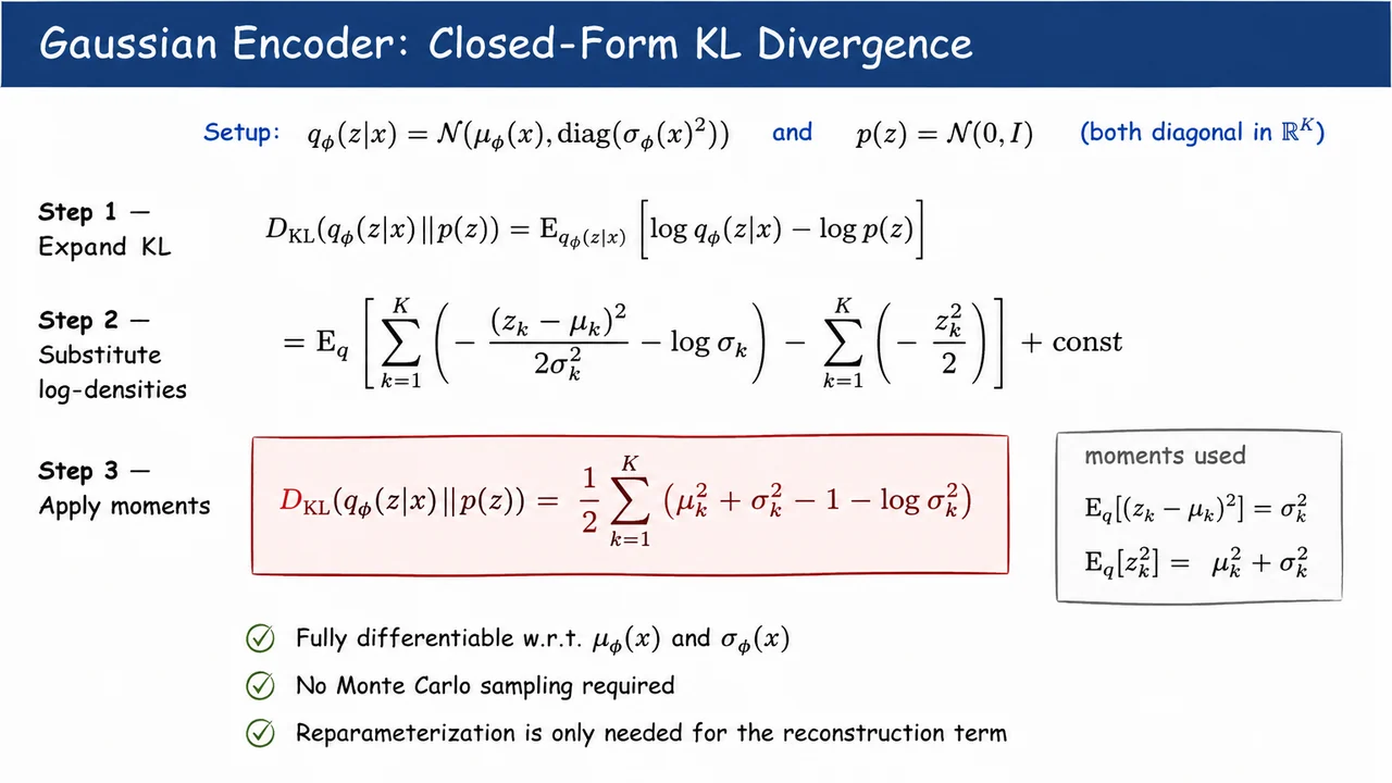
Start from the definition:
Because both distributions factorize across latent dimensions, their log-densities are sums over coordinates. Suppressing constants that will cancel or collect into dimension-independent terms, we can write
Here and mean the -th encoder outputs for the current datapoint . The expectation is still with respect to , but now only simple Gaussian moments are needed. Under ,
Substituting these moments and simplifying gives the exact closed form:
This expression is worth reading term by term. The penalty discourages the approximate posterior from shifting its mean far away from the prior mean . The combination
penalizes the posterior variance for deviating from the prior variance . It is minimized at , where it equals . Thus each latent coordinate pays no KL cost only when
meaning matches the prior along that coordinate.
A crucial practical point is that this KL term is fully differentiable and sampling-free. We do not need to draw to estimate it, and we do not need the reparameterization trick for this part of the objective. Gradients can flow directly through the encoder outputs and , or more commonly through and , since neural networks typically output log-variance for numerical stability.
This exactness also clarifies an important failure mode. Because the KL term pushes toward , a powerful decoder may learn to reconstruct well while ignoring . In that case the encoder can choose and , making the KL nearly zero. This is one view of posterior collapse: the approximate posterior becomes almost identical to the prior, so the latent code carries little information about .
There are a few assumptions hiding inside the neat formula:
The visual below condenses the derivation into the three essential moves: expand the KL definition, substitute the diagonal Gaussian log-densities, and apply the two Gaussian moment identities. The boxed expression is the quantity that appears directly in a VAE implementation.
It also separates the computational roles of the two ELBO terms. The KL side is analytic and deterministic; the reconstruction side still requires samples from , which is where the reparameterization trick from the previous section becomes necessary.
Having handled the KL term for a Gaussian encoder, the remaining piece of the ELBO is the part that asks a simple but crucial question: if we sample a latent code from the encoder, how well can the decoder explain the original observation? This is the reconstruction term,
It is often implemented as a mean-squared error loss, but that is not merely a convenient engineering choice. Under a Gaussian decoder assumption, MSE falls directly out of the likelihood model.
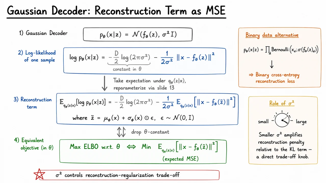
Assume the decoder defines a conditional Gaussian distribution over observations:
Here is the decoder network output, interpreted as the mean of the conditional distribution over . The variance says that, given , each observed dimension is corrupted by independent isotropic Gaussian noise with the same variance . This is a modeling assumption: it is reasonable for continuous-valued data after suitable normalization, but it is not automatically appropriate for binary pixels, counts, categorical variables, or perceptually structured image data.
For one latent sample , the Gaussian log-likelihood is
where is the dimensionality of . The first term is the Gaussian normalization constant. If is fixed, it does not depend on the decoder parameters . The second term is the squared reconstruction error, scaled by . Therefore, maximizing the Gaussian likelihood pushes toward in squared-error distance.
Inside the VAE, however, is not a single deterministic code. It is drawn from the approximate posterior , so the ELBO uses the expected log-likelihood:
Using the reparameterization trick, we usually write the sampled latent variable as
so the reconstruction term becomes an expectation over noise injected through a differentiable transformation. This is what lets gradients flow not only into the decoder parameters , but also back into the encoder parameters .
If is treated as a fixed hyperparameter, then maximizing the reconstruction term with respect to is equivalent to minimizing
up to a constant and a positive scaling factor. This is the precise sense in which the Gaussian decoder gives rise to expected MSE as the reconstruction loss. In practice, this expectation is usually approximated with one or a few Monte Carlo samples of per datapoint.
There are two subtle points worth keeping separate. First, the constant term
can be dropped only when is fixed. If is learned, that term matters; otherwise the model could change its variance without paying the correct likelihood normalization cost. Second, although dropping constants is harmless for optimizing , the reconstruction expectation still depends on through . So the encoder is trained not only to match the prior through the KL term, but also to choose latent distributions that allow accurate reconstructions.
The variance also has an important practical interpretation. In the full ELBO,
the reconstruction penalty is scaled by . Smaller makes reconstruction errors more expensive relative to the KL regularizer; larger softens the reconstruction pressure and makes the KL term comparatively more influential. Thus acts like a reconstruction–regularization trade-off knob, much like the weighting coefficient in a -VAE, though it arises from the likelihood model itself.
This likelihood choice also helps explain a classic VAE failure mode: blurry reconstructions. A Gaussian decoder trained with squared error is rewarded for predicting conditional means. When the posterior or decoder is uncertain among several plausible outputs, averaging them can produce visually smooth or blurry samples. This is not just an optimization artifact; it is partly a consequence of the assumed observation model. For binary data, a more appropriate decoder is often Bernoulli,
which leads to a binary cross-entropy reconstruction term rather than MSE.
The visual below condenses this derivation into a chain: start from the Gaussian decoder, expand the log-likelihood, take the expectation under the encoder distribution, and then drop the -constant terms to reveal the expected MSE objective. The key algebraic move is that the squared Euclidean error appears directly inside the Gaussian log-density.
It also highlights the modeling choices surrounding the derivation: the reparameterized sample is what makes the expected reconstruction loss trainable by backpropagation, the Bernoulli alternative reminds us that MSE is not universal, and the note about previews how the reconstruction term will be balanced against the KL divergence in the full VAE objective.
Now that the Gaussian decoder has turned the reconstruction term into something as familiar as squared error, we can finally assemble the pieces into the objective that is actually optimized in a VAE. The important point is that the VAE loss is not just reconstruction error with noise injected into the latent space. It is a variational lower bound with two coupled responsibilities: explain each datapoint well through the decoder, while keeping the encoder’s approximate posterior close enough to the prior that generation remains possible.
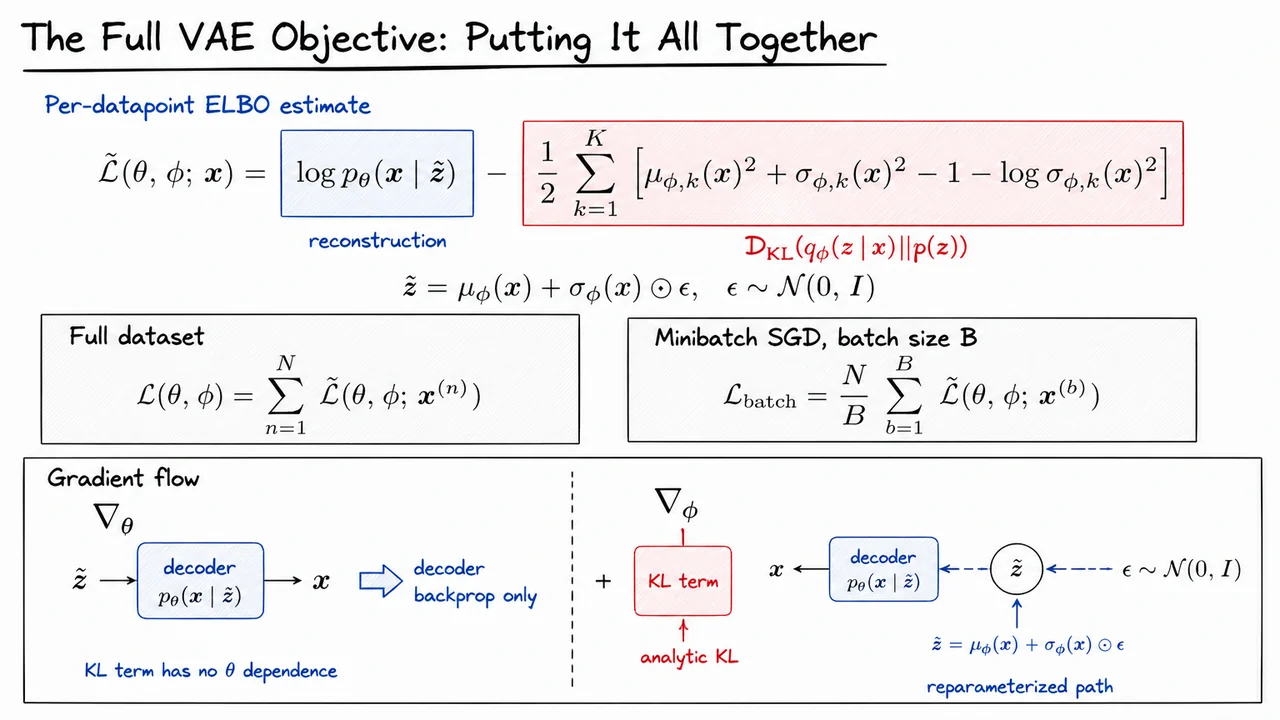
For a single datapoint , the ELBO is
The first term rewards latent samples that allow the decoder to assign high probability to the observed datapoint. The second term penalizes the encoder distribution for drifting too far from the prior , usually . This is what makes the latent space usable at generation time: after training, we want to sample , not from some fragmented collection of unrelated encoder distributions.
In practice, the expectation in the reconstruction term is estimated with samples. With the reparameterization trick, we write
This separates the randomness from the encoder parameters . Instead of sampling from a distribution whose parameters depend on in a way that blocks ordinary backpropagation, we sample parameter-free noise and transform it differentiably. That is the key technical move that allows gradients from the decoder’s reconstruction likelihood to flow backward through , then into and .
Using one Monte Carlo sample , the per-datapoint stochastic ELBO estimate becomes
Here the KL term has been written in closed form for the common diagonal Gaussian encoder
with standard normal prior . This analytic KL is one of the conveniences of the classical VAE setup. It avoids adding more sampling noise to the objective and gives a direct regularizing signal to the encoder.
A useful way to read the objective is as a controlled compromise:
This compromise is also where many VAE failure modes originate. If the KL penalty dominates too early, the encoder may learn for all , causing posterior collapse: the latent variable carries little information, and the decoder behaves almost like an unconditional model. If the reconstruction term dominates, the model may encode datapoints very precisely but produce a latent space that does not match the prior, making prior samples poor. With Gaussian decoders, another common issue is blurry reconstructions, because maximizing a pixelwise Gaussian likelihood often encourages conditional means rather than sharp, multimodal outputs.
For a dataset , training maximizes the sum of per-datapoint estimates:
Since full-dataset optimization is usually impractical, we use minibatches. For a batch of size , an unbiased estimate of the full objective is
Many implementations omit the factor when optimizing an average loss, because it only rescales the gradient for a fixed dataset and can be absorbed into the learning rate. What matters conceptually is that the minibatch objective estimates the same dataset-level ELBO. Also note the sign convention: derivations usually maximize the ELBO, while code often minimizes the negative ELBO, sometimes reported as reconstruction loss plus KL penalty.
The gradient dependencies are asymmetric but tightly coordinated. The decoder parameters appear only inside the likelihood term , so is ordinary decoder backpropagation. The encoder parameters , however, receive two kinds of signal: an analytic KL gradient that pushes toward zero and toward one, and a reconstruction gradient that flows through the reparameterized latent sample . This is why the full VAE objective trains encoder and decoder jointly rather than treating inference and generation as separate procedures.
The visual below condenses this entire training objective into its two main colored pathways. The blue reconstruction path represents the stochastic, reparameterized route from encoder outputs through into the decoder likelihood. The red KL path represents the closed-form regularizer acting directly on the encoder’s Gaussian parameters.
It also separates the three levels at which the same idea appears: the per-datapoint ELBO estimate, the full-dataset sum, and the minibatch estimator used in SGD. That hierarchy is worth keeping in mind before moving to the training algorithm: implementation is mostly bookkeeping, but the bookkeeping must preserve these two terms and their gradient paths.
Now that the ELBO has been assembled into a reconstruction term minus a regularization term, the remaining question is operational: what exactly happens during one training iteration? A VAE can look conceptually complicated because it contains an encoder, a decoder, a latent random variable, and a variational objective. But the actual training loop is quite close to ordinary minibatch SGD once we express the stochastic latent sample in a differentiable way.
For each datapoint in a minibatch, the encoder produces the parameters of an approximate posterior distribution,
The diagonal Gaussian assumption is doing a lot of work here. It makes sampling cheap, makes the KL divergence against the standard normal prior analytic, and gives us a simple parameterization for uncertainty in each latent dimension. In implementations, the network often predicts , or logvar, rather than directly, because the variance must remain positive and because log-variance is numerically more stable.
The central step is the reparameterized forward pass. Instead of sampling directly from , we sample parameter-free noise
and construct
This turns the random draw into a deterministic differentiable function of , , and external noise . That distinction is essential: gradients cannot flow through “sample from this distribution” in the usual backpropagation sense, but they can flow through addition, multiplication, and neural network outputs. The randomness remains, but it has been isolated from the parameters.
Once is sampled, the decoder evaluates the likelihood of reconstructing from that latent code:
This term depends on the chosen observation model. For binarized MNIST, it is usually a Bernoulli log-likelihood. For continuous data, one often uses a Gaussian likelihood, sometimes with fixed variance. This modeling choice matters: a simple Gaussian decoder trained with squared-error-like losses often encourages averaged reconstructions, which is one reason VAEs can produce blurry samples compared with adversarial models.
The KL term is computed analytically for each example because both and the prior are Gaussian. For a -dimensional diagonal posterior,
This term penalizes approximate posteriors that drift too far from the prior. Intuitively, it asks the encoder to use latent space economically: encode information only when it improves reconstruction enough to justify the cost. That tradeoff is powerful, but it also creates one of the most important VAE failure modes: posterior collapse. If the decoder is expressive enough to model the data without using , optimization may drive close to , making the latent code nearly uninformative.
Putting the two pieces together, a single-sample Monte Carlo estimate of the per-example ELBO is
Using one latent sample per datapoint is common because the minibatch itself already provides stochasticity, and the reparameterized gradient estimator usually has manageable variance. More samples can reduce variance, but they also increase computation; in standard VAE training, one sample is often a good tradeoff.
For a minibatch of size , the objective is typically written as an unbiased estimate of the full-data ELBO:
The factor appears if we are estimating the sum of ELBOs over the dataset. Many software implementations instead optimize the minibatch mean and omit ; this changes the scale of the loss and therefore the effective learning rate, but not the location of the optimum. The sign convention is another common source of bugs: mathematically we maximize the ELBO, while most deep learning libraries minimize losses, so implementations often minimize
Both parameter sets are updated from the same scalar objective. The decoder parameters receive gradients through the reconstruction likelihood. The encoder parameters receive gradients through two paths: directly through the analytic KL term, and indirectly through into the reconstruction term because of the reparameterization trick. In gradient-ascent form,
In practice, these are simultaneous optimizer updates, usually performed by Adam or a related adaptive method.
The key algorithmic pattern is therefore:
The visual that follows compresses this whole training iteration into a pseudocode-style view. The highlighted latent-sampling line is the computational heart of the VAE: it is what converts a stochastic latent-variable model into something compatible with backpropagation. The highlighted KL line emphasizes the other major simplification: for the standard Gaussian prior and diagonal Gaussian encoder, this part of the ELBO does not need Monte Carlo estimation.
The update lines at the bottom summarize the most important implementation detail: and are optimized together using the same minibatch ELBO estimate. The gradient notes make explicit where each derivative flows— through the decoder likelihood, and through both the analytic KL and the reparameterized reconstruction path.
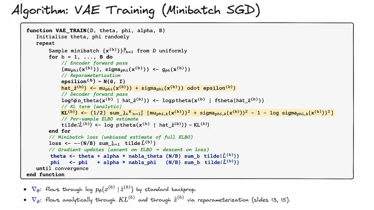
After the training loop is written down, the VAE can still feel slightly abstract: we say “encode, sample, decode, add KL, backpropagate,” but it is worth seeing what those words mean for one concrete datapoint. Let us trace a single minibatch element: a binarized MNIST digit, say a handwritten , represented as . The pixels are binary, so the natural decoder likelihood is a product of Bernoulli distributions over pixels, with the decoder producing logits or probabilities for each of the 784 coordinates.
For this worked example, suppose the latent space is only two-dimensional, . This is much smaller than we would typically use for high-quality generation, but it is ideal for understanding the mechanics. The encoder network maps the image to the parameters of a diagonal Gaussian approximate posterior,
For our particular image, assume the encoder outputs
These numbers have a simple interpretation. The encoder believes that, for this digit, plausible latent codes are centered near , with less uncertainty in the first coordinate than the second. The diagonal covariance assumption means the two latent dimensions are conditionally independent under , which makes both sampling and the KL term cheap. This assumption is computationally convenient, but it is also restrictive: if the true posterior has strong correlations between latent dimensions, a diagonal Gaussian encoder cannot represent them directly.
Now we need a latent sample. A naive expression would be
but this hides a problem: the sampling operation depends on , and we want gradients to flow through the sampled latent code into the encoder. The reparameterization trick rewrites the sample as a deterministic differentiable function of , , and external noise that does not depend on :
If, for this forward pass, we draw
then the latent sample is
The important point is not just the numerical value. It is the computational path: is now differentiable with respect to both and . The randomness has been isolated in , while the dependence on encoder parameters remains inside ordinary differentiable arithmetic.
The decoder then maps back to Bernoulli parameters for the 784 pixels. For a binary image, the reconstruction log-likelihood has the form
where is the decoder’s predicted probability that pixel is on. Suppose this particular decoder evaluation gives
This term rewards reconstructions that assign high probability to the observed binary pixels. Since it is a log probability over 784 dimensions, a negative value is expected. What matters during optimization is whether changing and makes this quantity less negative on average while maintaining a reasonable latent posterior.
The regularizer is the KL divergence from the approximate posterior to the standard normal prior . Because both distributions are diagonal Gaussians, the KL has a closed form:
Plugging in the two latent dimensions gives
This number measures how much the encoder’s posterior for this example deviates from the prior. Large means, very small variances, or very large variances all tend to increase the KL. Intuitively, the KL penalizes the encoder for using latent codes that are too specialized or too far from the standard normal geometry that the decoder will later sample from at generation time.
Combining the reconstruction term and the KL term gives the single-sample Monte Carlo estimate of the ELBO:
Training maximizes this quantity, or equivalently minimizes its negative. The gradients split cleanly. Parameters receive gradients through the decoder likelihood. Parameters receive gradients in two ways: directly through the analytic KL term, and indirectly through the reconstruction term via
This is why the reparameterization trick is not a cosmetic rewrite; it is what makes the reconstruction part of the objective train the encoder using standard backpropagation.
There are already hints of common VAE failure modes in this tiny example. If the KL pressure is too strong, the encoder may learn and for most inputs, making nearly equal to the prior; then the decoder may ignore , a phenomenon known as posterior collapse. Conversely, if the decoder likelihood is too simple or the latent representation is too compressed, reconstructions may average over plausible outputs, producing the characteristic blurriness associated with VAEs on continuous-valued images. Even in binarized MNIST, where Bernoulli likelihoods are relatively well matched to the data, the balance between reconstruction accuracy and latent regularity is the central tension.
The visual below condenses this entire forward pass into one computation graph: a binarized image enters the encoder, the encoder emits and , external Gaussian noise is injected through the reparameterization equation, and the resulting is decoded into a Bernoulli reconstruction score. The KL calculation is separated because it does not require sampling; once and are known, its value follows analytically.
It also highlights the gradient story. The decoder parameters are trained through the reconstruction likelihood, while the encoder parameters are trained both by the closed-form KL and by the decoder loss through . That combination—one stochastic but reparameterized reconstruction path plus one deterministic Gaussian KL path—is the practical core of VAE training.
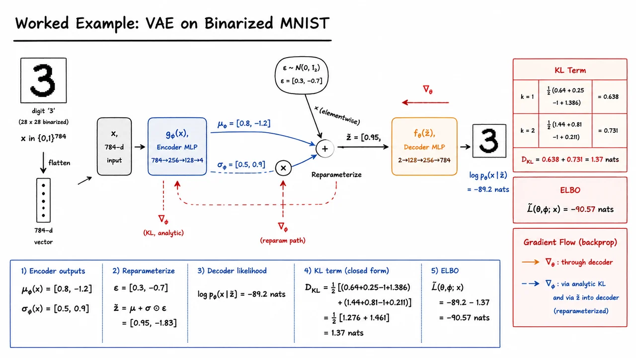
After walking through a single numerical forward pass, the natural next question is: what does all this optimization actually buy us? A VAE is not trained merely to reconstruct individual inputs. It is trained to shape a latent space in which encoding, sampling, decoding, and interpolation all behave coherently. The empirical test is therefore twofold: whether the latent variables organize semantic information, and whether samples drawn from the prior decode into plausible observations.
A useful diagnostic is to look at the encoder means . Recall that the encoder produces an approximate posterior
so is the “central” latent representation assigned to . If we train a VAE on MNIST with only two latent dimensions, we can scatter-plot for thousands of test images. This is not just a visualization trick: in , the entire learned latent geometry is visible.
What we typically see is a semantically structured but overlapping latent space. Digits of the same class tend to occupy nearby regions, because the decoder can more easily reconstruct similar digits from nearby latent codes. But the clusters are not perfectly separated. That is expected, and in fact desirable: the VAE objective does not ask for a discriminative classifier. It balances reconstruction quality against proximity to the prior . The KL term discourages the encoder from carving the latent space into isolated islands far from the origin.
This is one of the central empirical signatures of VAEs: nearby latent points decode to nearby-looking outputs. If two codes and are close in latent space, then the decoder usually maps them to visually similar digits. This continuity comes from both the neural decoder and the regularization imposed by the prior. Without the KL penalty, an autoencoder can learn a jagged, disconnected latent representation where interpolation may pass through meaningless regions. With the VAE objective, the model is pressured to make the latent space usable under samples from a simple distribution.
Generation then becomes conceptually simple. We sample
and decode it using , often parameterized by a neural network . For MNIST, the generated samples are usually recognizable as digits. However, they often look soft or blurry, especially compared with real handwritten digits. This is not merely an implementation flaw; it reflects a modeling assumption.
In the common Gaussian decoder setting,
maximizing likelihood encourages the decoder output to approximate a conditional mean. If several plausible sharp images correspond to nearby latent explanations, the mean of those possibilities may average edges, strokes, and fine details. The result is a digit that is semantically correct but visually smoothed. This is one reason VAEs are often said to trade sample sharpness for a well-behaved likelihood objective and structured latent space.
Interpolation is another revealing experiment. Given two test images and , we encode them to their posterior means and linearly interpolate:
Decoding for increasing often produces a smooth morph, such as a digit gradually becoming an . This matters because it suggests that the model has learned more than memorized examples. It has learned a continuous latent manifold where semantic transformations correspond to smooth movement in .
Quantitatively, we still judge the model through the ELBO. Kingma and Welling reported a test-set bound around
for a stronger VAE configuration with a -unit MLP and latent dimensions. A two-dimensional latent space is excellent for visualization, but it is capacity-limited: many details needed to explain the data must be compressed away. With , the approximate posterior can retain more information while still being regularized toward the prior, typically yielding a better ELBO.
The main takeaways are:
The visual below consolidates these empirical checks into one picture: a two-dimensional latent scatter to expose structure, generated samples to test the prior-to-decoder path, interpolation to test continuity, and an ELBO curve to connect the qualitative behavior back to the optimization objective.
It is important to read the panels together. A clean latent scatter alone does not guarantee good generation, and good-looking reconstructions alone do not guarantee a useful prior. The strength of the VAE is that these behaviors are coupled by the ELBO: reconstruction encourages informativeness, KL regularization encourages global structure, and the resulting model supports both sampling and smooth latent manipulation.
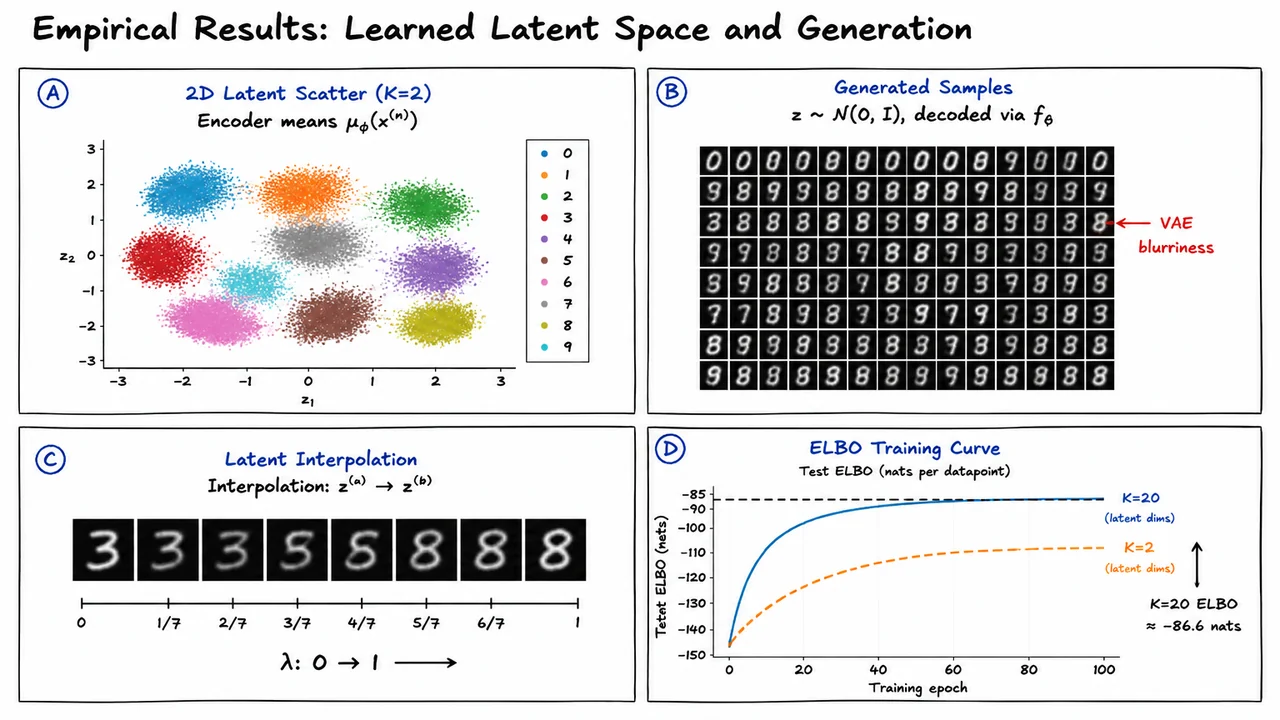
The latent traversals and generated samples we just looked at are the success case for VAEs: the encoder has learned a meaningful map from data into latent variables , and the decoder has learned to use those variables to control semantic properties of the output. But this behavior is not guaranteed by the VAE objective. In fact, one of the most important VAE failure modes is that the model can optimize the ELBO while learning a latent space that carries almost no information at all.
Recall that for a single datapoint , the ELBO is
This objective creates a negotiation between two incentives. The reconstruction term rewards the encoder for placing information about into , because a useful helps the decoder assign high likelihood to the observed data. The KL term pushes in the opposite direction: it rewards the approximate posterior for staying close to the prior , usually a standard Gaussian. If a latent dimension is not useful enough to improve reconstruction, the cheapest solution is to make that dimension look exactly like prior noise.
Posterior collapse occurs when this cheap solution becomes the dominant one. For some latent dimension , collapse means
When this happens, carries essentially no information about . Sampling from the encoder is no different from sampling it from the prior. The encoder may still output a mean and variance, but if those parameters match the prior for every input, then the latent coordinate has become statistically independent of the data. In practice, one often observes the KL term quickly shrinking toward zero early in training, long before the decoder has learned a useful conditional generative model.
The most dangerous case arises when the decoder is powerful enough to model the data distribution without using . Suppose the decoder becomes effectively -independent:
Then the reconstruction term no longer depends on the encoder distribution:
At that point, there is no reconstruction benefit to encoding information in . The only remaining pressure on the encoder is the KL penalty, and the KL is minimized by setting
This is why posterior collapse is not merely a transient optimization accident; it can be a stable fixed point of the ELBO. Once the decoder can explain on its own, the encoder is actively rewarded for becoming uninformative.
This failure mode is especially common with highly expressive decoders: autoregressive PixelCNN-style image decoders, strong Transformer decoders, or LSTM decoders for language. These models can often predict local structure from previously generated pixels or tokens so well that the global latent variable becomes unnecessary. The decoder learns a strong marginal model , while the intended conditional model effectively ignores its conditioning signal.
There is a subtle but important distinction here. Posterior collapse does not necessarily mean the model has poor likelihood. A collapsed VAE may still assign decent likelihood to data if the decoder is strong enough. The failure is that the model no longer behaves like a useful latent-variable model. The latent space will not organize examples semantically, interpolations become meaningless, and downstream uses of —compression, representation learning, controllable generation—break down.
A useful diagnostic is to monitor the per-dimension KL terms during training. In a healthy VAE, some latent dimensions usually develop positive KL: the model is “paying” bits to transmit information through . In a collapsed model, many or all dimensions have KL near zero:
The visual below compactly summarizes both the training symptom and the mechanism. On the left, the key signal is the KL trajectory: a useful latent space requires the KL to rise above zero, while collapse appears as a flat line near zero. On the right, the information-flow picture emphasizes the cause: the path through is no longer used, so the encoder has no reason to encode input-specific information.
Read the diagram as a warning about the ELBO’s incentives. The KL term is not just a harmless regularizer; when the decoder can reconstruct or predict without , the KL penalty can make “ignore the latent variable” the easiest optimum. This sets up the next failure mode as well: even when VAEs do use , the probabilistic reconstruction objective can still produce overly smooth or blurry samples.
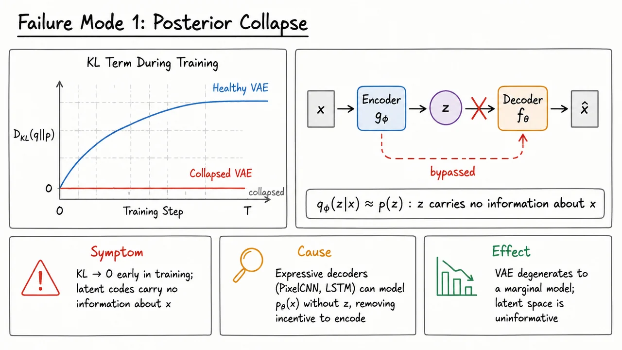
After posterior collapse, it is tempting to think the main danger in VAEs is that the latent variable becomes unused. But even when the latent code is used, VAEs often exhibit another characteristic failure mode: reconstructions look smooth, washed out, or “average-looking.” This is not merely an implementation artifact. It follows directly from the likelihood model we usually choose and from the way the ELBO trades reconstruction fidelity against latent regularity.
The standard VAE decoder is often written as a Gaussian likelihood,
where is the decoder’s predicted image mean. If is fixed, maximizing the reconstruction log-likelihood is equivalent, up to constants and scaling, to minimizing a pixel-wise squared error:
This is the key point: squared error rewards conditional averages. If there are multiple plausible sharp reconstructions compatible with the latent uncertainty, the prediction that minimizes expected squared error is not necessarily one of those sharp possibilities. It is their mean.
More precisely, under an MSE objective, the optimal point estimate is a conditional expectation. In the VAE setting, because reconstructions are averaged over samples from the approximate posterior , the effective optimum behaves like
This is harmless when the posterior mass corresponds to a narrow set of nearly identical decodings. But it becomes visually damaging when the plausible decodings are multimodal. For example, if a digit could plausibly have a stroke slightly to the left or slightly to the right, the pixel-wise average puts mass in both places weakly. The resulting image is not a realistic digit from either mode; it is a blurred compromise between them.
This is why VAE blurriness is often described as an “averaging” phenomenon. The decoder is not explicitly trying to blur images. Rather, the Gaussian likelihood says that deviations in pixel space are penalized quadratically, independently across pixels. Under this geometry, a soft gray pixel halfway between black and white can be preferable to committing to the wrong sharp value. The model is rewarded for being safe under uncertainty, not for producing a sample that lies on the manifold of visually crisp images.
The KL term compounds the problem. Recall the single-example ELBO:
The reconstruction term wants to encode enough information to reconstruct sharply. The KL term pushes toward the prior, typically . This pressure discourages highly concentrated, highly informative posteriors. In effect, it can broaden , increasing the range of latent samples that the decoder must handle for the same input.
So even before collapse, the model is caught between two forces:
This tradeoff is part of what makes VAEs attractive as generative models: their latent spaces are usually smooth, interpolatable, and mode-covering. But the price is that their samples and reconstructions can look less sharp than those from models trained with perceptual or adversarial criteria.
GANs fail in almost the opposite direction. A GAN discriminator does not ask whether each pixel is close to a target under squared error. It asks whether the generated sample looks like it came from the real data distribution. A blurry average of several plausible images is often easy for a discriminator to reject, so adversarial training strongly penalizes unrealistic smooth compromises. This is why GAN samples are frequently sharper. However, that sharpness comes with a different failure mode: mode dropping. The generator can learn to produce a subset of highly realistic samples while ignoring other regions of the data distribution.
This comparison is useful because it separates two notions that are often conflated: sharpness and coverage. VAEs tend to cover the data distribution more systematically because the likelihood objective assigns probability mass broadly and the latent prior encourages global organization. GANs tend to produce sharper samples because adversarial feedback rewards realism, but they may cover fewer modes. Neither objective is universally better; they encode different preferences.
Within the VAE framework, there are several ways to reduce blurriness, each changing the balance of this tradeoff. One can replace pixel-wise MSE with a perceptual loss, measuring reconstruction error in the feature space of a pretrained network rather than raw pixels. One can add an adversarial term, producing hybrid models such as VAE-GANs. Or one can reduce the decoder variance , effectively increasing the weight of reconstruction accuracy relative to the KL term. But these interventions are not free: they can destabilize training, weaken likelihood interpretation, or reduce the smoothness and coverage properties that motivated VAEs in the first place.
The visual below compresses this story into a side-by-side comparison. On the VAE side, a broad approximate posterior sends multiple latent samples through the decoder; averaging their plausible outputs produces a blurry mean. In the center, the loss comparison highlights the mechanism: Gaussian likelihood/MSE encourages mode coverage but tolerates visual averaging, while adversarial training penalizes unrealistic blur.
The GAN side then illustrates the complementary behavior: samples can be crisp because the discriminator enforces perceptual realism, but the generated examples may become repetitive, signaling missing modes. This is the central takeaway: VAE blurriness is not accidental; it is a consequence of averaging under latent uncertainty, amplified by KL regularization. GAN sharpness solves that visual problem by changing the objective, but introduces its own coverage failure mode.
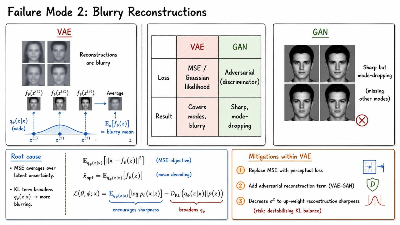
After seeing why VAEs can produce blurry reconstructions, it is tempting to ask whether we can tune the objective to prefer a different kind of representation. The standard VAE is already balancing two competing goals: reconstruct the input well, while keeping the approximate posterior close to a simple prior. Beta-VAE makes this trade-off explicit by introducing a single scalar knob, , that controls how strongly we penalize information stored in the latent variable.
Recall the standard VAE objective for one data point :
The first term rewards good reconstruction. The second term regularizes the encoder distribution , usually pushing it toward a simple prior such as
Beta-VAE modifies only one thing: it multiplies the KL term by :
When , this is exactly the usual VAE ELBO:
For , however, the objective is no longer the standard ELBO on . It is better understood as a rate–distortion trade-off: the reconstruction term is the distortion, while the KL term controls the rate, meaning how much information about can be transmitted through . Increasing makes latent information more expensive.
This pressure can encourage disentanglement. The prior is factorized:
So if the encoder is heavily penalized for deviating from this prior, it is encouraged to use latent dimensions in a way that remains close to independent, standardized Gaussian coordinates. Under the common diagonal Gaussian encoder,
the KL term decomposes across dimensions:
This expression makes the effect of concrete. Unless a latent dimension helps explain real variation in the data, the model is rewarded for keeping
In other words, unused or weakly useful dimensions are pushed back toward pure prior noise. Dimensions that remain active must “earn their keep” by improving reconstruction enough to compensate for the larger KL penalty.
The intuitive hope is that each active latent coordinate will specialize in a distinct factor of variation: one dimension for shape, another for scale, another for rotation, another for lighting, and so on. Empirically, this often happens on controlled datasets such as dSprites or 3DShapes, where the underlying generative factors are relatively clean and independent. Values such as can produce latents where traversing one coordinate changes one semantic factor while leaving others mostly fixed.
But this is not magic, and it is important not to overstate the guarantee. Disentanglement depends on several assumptions:
So Beta-VAE is best understood as a useful bias, not a theorem that semantic factors will automatically emerge.
The cost is also direct: as increases, reconstruction quality usually decreases. The decoder receives less information about the particular input , because the encoder is more constrained to keep close to . This can worsen the same reconstruction problems we discussed earlier: less detail, more averaging, and potentially blurrier outputs. Beta-VAE therefore trades fidelity for structure.
A useful way to summarize the idea is to imagine as a dial. At , we have the ordinary VAE objective: better reconstructions, but latent dimensions may be entangled. As grows, the KL term becomes more dominant, pushing the posterior closer to the independent Gaussian prior. The latent space may become more axis-aligned and interpretable, but the reconstructions become less faithful.
The visual below consolidates this trade-off: the left side represents the standard VAE regime, where latent coordinates can mix multiple factors; the center emphasizes the modified objective and the -controlled tension between reconstruction and regularization; the right side represents the Beta-VAE regime, where dimensions are encouraged to separate factors such as shape and scale, but with degraded reconstruction quality as the price.
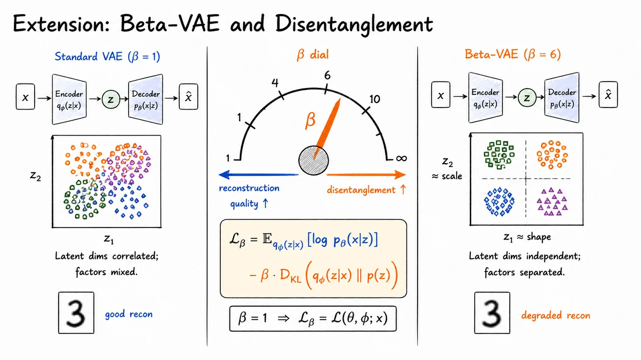
After seeing how -VAE deliberately reshapes the latent space by changing the strength of the KL penalty, it is useful to step back and ask a broader question: what kind of generative model is a VAE, and what does it trade away compared with other families? VAEs are often introduced alongside GANs and normalizing flows because all three learn to generate samples from data, but they make very different compromises about likelihoods, latent variables, optimization, and sample quality.
The VAE starts from an explicitly probabilistic story. We assume a latent variable , usually , and a decoder likelihood . The marginal likelihood is
but this integral is generally intractable for neural decoders. The VAE therefore optimizes the Evidence Lower Bound:
This objective is not merely a training trick. It encodes the core VAE design philosophy: learn to reconstruct data through a latent bottleneck while keeping the approximate posterior close to a simple prior. That KL term is exactly what gives VAEs their unusually useful latent geometry. Nearby points in latent space tend to decode to semantically related outputs, interpolation is meaningful, and the latent representation can support downstream tasks such as clustering, semi-supervised learning, and controllable generation.
But the same structure also explains common VAE weaknesses. Because the decoder is trained through a likelihood term, the model is often rewarded for predicting averages under uncertainty. With Gaussian pixel likelihoods, this can produce blurry reconstructions: if multiple sharp images are plausible, the conditional mean may lie between them. And when the decoder is too powerful, the model may ignore entirely, producing posterior collapse, where and the latent code carries little information about . In other words, the VAE’s principled probabilistic objective is also the source of its characteristic compromises.
GANs sit at almost the opposite end of the spectrum. A GAN generator maps noise to a sample , while a discriminator tries to distinguish generated samples from real data. The classical minimax objective is
This adversarial formulation can produce extremely sharp and realistic samples because the generator is trained to fool a learned critic rather than to maximize a pixelwise likelihood. However, GANs usually do not provide tractable likelihoods, and their latent space is not regularized by an inference model in the VAE sense. There is no built-in encoder , no ELBO, and no direct estimate of . As a result, GANs are powerful image synthesizers but less naturally suited to probabilistic inference or structured representation learning.
Normalizing flows take a third route: they preserve exact likelihoods by making the generative map invertible. A flow defines an invertible transformation between data and latent variables , allowing density evaluation through the change-of-variables formula:
This is a major advantage: unlike VAEs, flows do not optimize a lower bound; unlike GANs, they can evaluate exact densities. But this exactness comes with architectural constraints. The transformation must be bijective, which usually forces the latent dimensionality to match the data dimensionality, . The model cannot freely compress data into a lower-dimensional semantic bottleneck in the way a VAE can. Flows are excellent density models, but their latent spaces are often less directly aligned with compact representation learning.
A useful way to summarize the comparison is to ask what each model gives you “for free” and what it makes difficult:
The key point is that there is no universally dominant model family. The right choice depends on whether the priority is sample realism, density evaluation, or latent representation structure. If the task is pure image synthesis, GAN-like models may be attractive. If exact log-likelihood is central, flows are compelling. If we care about a learned latent space that is smooth, regularized, and useful for inference or downstream prediction, VAEs remain especially important.
The visual comparison that follows condenses these trade-offs into the axes that matter most: objective, sampling procedure, density evaluation, latent structure, and sample quality. Notice in particular the contrast between the VAE’s ELBO-based density estimate and the flow’s exact likelihood, as well as the contrast between the VAE’s KL-regularized latent space and the more weakly structured latent variables used by GANs.
The highlighted cells emphasize the central lesson: VAEs are not simply “worse GANs” because their samples can be blurrier, nor are they merely “approximate flows” because they optimize a bound rather than exact likelihood. Their distinctive strength is the combination of a probabilistic training objective with a structured latent representation, which is precisely why they remain a foundational tool for representation learning, semi-supervised modeling, and latent-variable inference.
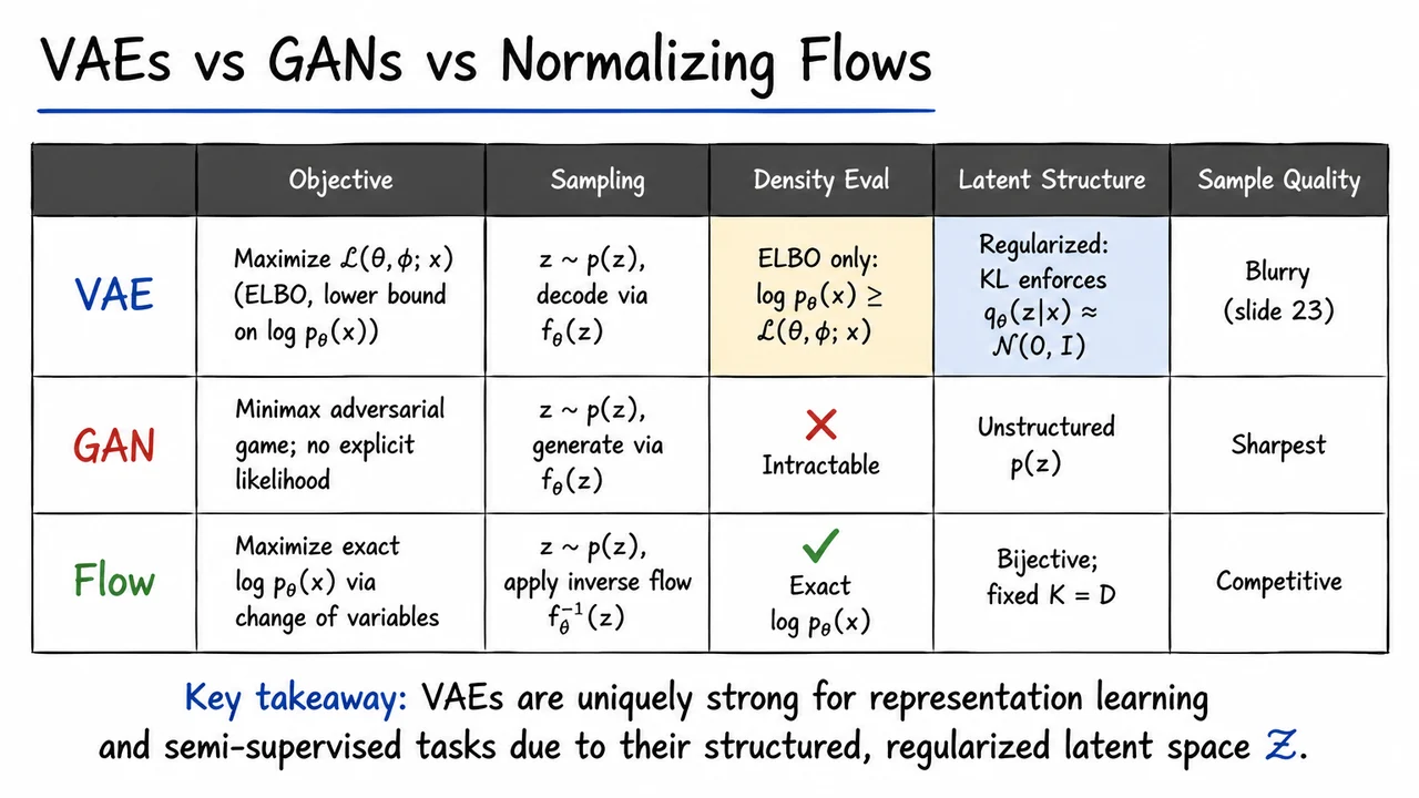
After comparing VAEs with GANs and normalizing flows in the abstract, it is useful to ground the discussion in a concrete empirical example. CelebA faces are a particularly good testbed: the images are structured enough that we can see semantic attributes—pose, hair, glasses, gender presentation, expression—but constrained enough that a moderately sized convolutional VAE can learn a meaningful latent representation.
Consider a convolutional VAE trained on roughly 200k CelebA images resized to RGB. The encoder maps an image through several convolutional layers and a fully connected layer to the parameters of a diagonal Gaussian posterior approximation,
with latent dimension . The decoder maps a latent vector back through a fully connected layer and transposed convolutional layers to a Gaussian mean image. In other words, the decoder is not directly producing a sharp image distribution in pixel space; it is producing the mean of a conditional Gaussian likelihood.
At training and reconstruction time, the latent sample is drawn using the reparameterization trick,
This matters because the encoder is not merely assigning each image to a deterministic code. It is learning a local distribution over plausible codes, regularized toward the prior . The VAE therefore has to balance two goals: preserving enough information to reconstruct the face, while keeping the aggregate latent geometry compatible with sampling from a simple Gaussian prior.
The first qualitative result is reconstruction. If we encode a real face, sample , and decode , the output is usually recognizable: identity, hair color, pose, and broad facial structure are often preserved. But the image is noticeably soft. This is not an incidental flaw of convolutional networks; it is tightly connected to the Gaussian likelihood and pixelwise squared-error reconstruction term. When multiple plausible high-frequency details could explain an input—exact hair strands, skin texture, eye highlights—the conditional mean averages over them. The result is the familiar VAE blur.
That blur is the qualitative price paid for a likelihood-based, mode-covering generative model with a simple reconstruction distribution. Unlike a GAN, which may learn sharp samples by matching an implicit distribution adversarially, the standard Gaussian VAE is explicitly rewarded for predicting an average pixel value under uncertainty. This is why simply training longer or increasing the latent dimension often does not remove the softness. To substantially change the visual character, one usually modifies the likelihood, the reconstruction loss, the decoder distribution, or introduces more expressive generative structure.
The second result is unconditional generation. If we sample
and decode , we obtain plausible faces rather than random noise. This is a key empirical validation of the VAE objective: the KL term has shaped the encoder’s latent codes so that regions likely under the prior correspond to meaningful decoded images. In a poorly regularized autoencoder, sampling a random latent vector would often land in “holes” between encoded training examples. In a well-trained VAE, the prior is encouraged to cover the learned manifold.
The third result is more subtle: the latent space often supports semantic arithmetic. Using posterior means as deterministic summaries of images, we may find relationships like
Decoding the resulting vector can produce a face that preserves the “woman” identity direction while adding the “glasses” attribute. This should not be interpreted as exact symbolic reasoning. The latent space is not guaranteed to contain perfectly linear, disentangled factors. But because the prior is smooth and the decoder is trained over a continuous latent domain, common attributes can become approximately represented as directions or subspaces.
A related phenomenon appears in interpolation. Given two images and , we can linearly interpolate between their posterior means,
Decoding points along this path often gives a smooth morph from one face to another. This is an important distinction between a VAE and a plain autoencoder: the latent space is not merely a lookup table of compressed examples. The ELBO’s KL term encourages neighboring latent regions to decode coherently, so linear paths can remain on or near the learned face manifold.
The visual below consolidates these four empirical anchors: reconstruction, unconditional generation, latent arithmetic, and interpolation. Read it as evidence for both sides of the VAE story. On one hand, the model has learned a semantically organized latent space where sampling, arithmetic, and smooth traversal are meaningful. On the other hand, the reconstructions and samples remain visibly soft, reminding us that the Gaussian decoder’s averaging behavior is not a cosmetic detail but a central modeling limitation.
This example is therefore a natural bridge into VAE extensions. Once we accept that the basic framework gives us a useful latent geometry but imperfect image fidelity, the motivation for richer decoders, hierarchical latents, discrete variables, perceptual losses, adversarial hybrids, and diffusion-style decoders becomes much clearer.
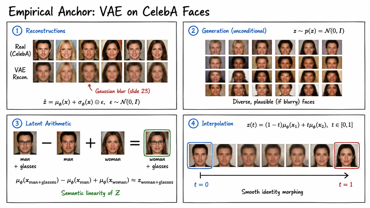
After seeing a standard VAE trained on CelebA, it is tempting to think of “the VAE” as one fixed architecture: an encoder produces a Gaussian latent distribution, a decoder reconstructs an image, and the ELBO balances reconstruction against KL regularization. But in practice, many of the most useful VAE variants keep this encode–sample–decode skeleton while changing one structural assumption in the probabilistic model or in the variational bound.
A useful way to organize the family is to ask: what exactly are we modifying?
These questions lead naturally to three important extensions: Conditional VAEs, Importance Weighted Autoencoders, and Vector-Quantized VAEs. They look different architecturally, but they are all still variations on the same principle: introduce latent structure, define a tractable training objective, and optimize an encoder–decoder system end-to-end.
The Conditional VAE, or CVAE, modifies the generative story by conditioning both inference and generation on observed side information . Instead of modeling , we model something closer to . The encoder becomes , the decoder becomes , and the prior may also depend on , giving the conditional ELBO
The intuition is simple but powerful: explains the part of the variation we already know, while captures the residual variation. For faces, might encode identity, expression, hair color, or a binary attribute such as “smiling.” At generation time, we fix , sample , and decode . This gives controlled generation: “generate a face with this attribute, while allowing the remaining details to vary.” The subtle assumption is that is available and meaningful during training; without paired supervision, the conditional structure cannot be learned directly.
The Importance Weighted Autoencoder, or IWAE, changes something different. It does not primarily add labels or alter the latent space type. Instead, it improves the variational objective. Recall that the ordinary ELBO is a lower bound on , derived by introducing an approximate posterior . The gap between the ELBO and the true log evidence is a KL divergence between and the exact posterior . IWAE tightens this bound by drawing samples from the encoder and forming an importance-weighted estimate:
For , this recovers the ordinary VAE ELBO. As increases, the bound becomes tighter, and under appropriate regularity assumptions,
This matters because the standard ELBO can be loose when the variational posterior is too simple. IWAE partially compensates by using multiple latent samples and letting high-importance samples dominate the estimate. But this improvement is not free. The tighter objective can produce more difficult optimization dynamics for the encoder parameters : as grows, the learning signal for the proposal distribution can degrade or become biased in practical gradient estimators. So IWAE improves the statistical bound, but it introduces a new optimization trade-off.
The VQ-VAE moves in a third direction: it replaces the usual continuous Gaussian latent variable with a discrete latent code. The encoder first outputs a continuous vector, but that vector is then snapped to the nearest entry in a learned codebook . The decoder receives the selected codebook vector rather than a sample from a continuous posterior. This is especially useful when the data has naturally discrete or symbolic structure: phonemes in speech, tokens in language-like representations, or repeated visual parts in images.
The difficulty is that nearest-neighbor lookup is not differentiable. A standard VAE relies on the reparameterization trick, for example , to backpropagate through stochastic sampling. VQ-VAE cannot use that trick directly because the latent choice is discrete. Instead, it typically uses a straight-through estimator: in the forward pass, the model uses the nearest codebook vector; in the backward pass, gradients are copied through the quantization operation as if it were approximately identity. This estimator is biased, but often effective. Another consequence is that, with a uniform prior over discrete codes, the KL term can collapse to a constant, so the objective is usually expressed through reconstruction plus codebook and commitment losses rather than the ordinary Gaussian KL penalty.
These three variants therefore form a compact hierarchy of interventions on the base VAE:
The visual below is meant to consolidate this taxonomy rather than introduce a new derivation. The table separates each model by the part of the VAE it changes: objective, key innovation, and trade-off. That framing is important because these extensions are not arbitrary architectural hacks; each corresponds to a different mathematical pressure point in the original VAE formulation.
The small diagrams beneath the table reinforce the same idea operationally. CVAE routes the label into both encoder and decoder, IWAE fans out multiple latent samples before combining them through an importance-weighted log average, and VQ-VAE inserts a codebook lookup between encoder and decoder. The common thread is that all three preserve the VAE’s central encode–latent–decode logic, while changing what the latent variable means or how its objective is optimized.
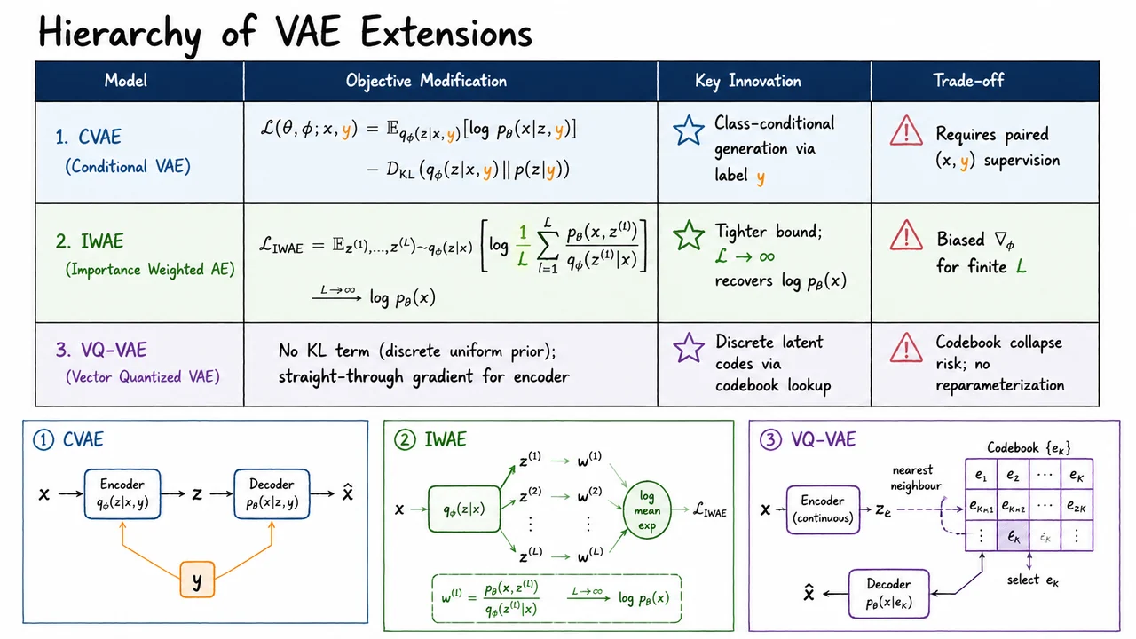
After seeing the hierarchy of VAE extensions, it is useful to step back and notice that most of the machinery we have introduced is not a collection of unrelated tricks. The latent-variable model, Jensen’s inequality, the KL gap, the reconstruction–regularization tradeoff, the reparameterization trick, and the Gaussian closed form are all different views of the same central object: the Evidence Lower Bound, or ELBO. The extensions change priors, posteriors, decoders, objectives, or training schedules, but the conceptual spine remains the same.
The starting point is the latent-variable likelihood
The difficulty is that this integral is usually intractable for a neural decoder . VAEs solve this not by evaluating the marginal likelihood directly, but by introducing an approximate posterior . This distribution is not part of the original generative model; it is an inference model, or encoder, trained to approximate the true posterior . Once we multiply and divide by , Jensen’s inequality gives the canonical ELBO form:
This is the most compact variational-inference statement of the VAE objective. It says: sample latent variables from the encoder, score them under the joint model, and subtract the cost of using the encoder distribution. Since it is a lower bound,
maximizing the ELBO is a surrogate for maximizing likelihood.
The same expression becomes more interpretable when we use the factorization . Then the ELBO decomposes as
This is the familiar reconstruction minus regularization form. The first term rewards latent codes that allow the decoder to explain . The second term penalizes the encoder posterior for drifting too far from the prior. This penalty matters because generation later samples , not . If the aggregate latent codes used during training live in regions of latent space that the prior rarely visits, generation will be poor even if reconstruction is good.
A third equivalent rewriting separates the KL term into entropy and prior energy:
This form emphasizes the connection to negative free energy and rate–distortion. The reconstruction term is a distortion-like quantity: how accurately can the latent representation explain the data? The KL-related terms control the information content and geometry of the representation. A low-entropy posterior can carry precise information about , but it pays a cost if it concentrates too sharply or moves away from the prior. A high-entropy posterior is cheaper and smoother, but may discard information needed for accurate reconstructions.
The fourth form reveals exactly when the bound is tight:
Equivalently,
So the gap between the ELBO and the true log evidence is not mysterious: it is exactly the KL divergence from the approximate posterior to the true posterior. The bound is tight if and only if
almost everywhere. This condition is important but subtle. In practice, the true posterior changes as changes, and the variational family may be too limited to represent it exactly. Thus the VAE optimizes a coupled problem: improve the generative model while simultaneously learning an amortized approximation to its posterior.
The fifth form is the one we actually implement for the standard Gaussian VAE. If
then we sample using the reparameterization trick
and use the closed-form Gaussian KL:
The practical training objective is therefore
This last expression is not a new objective; it is the computationally usable version of the same ELBO under Gaussian assumptions. The reparameterization trick is what makes gradients with respect to low-variance and compatible with backpropagation: randomness is pushed into , while and remain differentiable functions of the encoder parameters.
Seen this way, the VAE is a unification of two tasks:
The strengths and failure modes follow directly from this unified objective. Posterior collapse occurs when the decoder becomes strong enough that the optimum can ignore , pushing close to and making the KL small but the latent code uninformative. Blurry reconstructions often arise when the likelihood model, such as a factorized Gaussian decoder, rewards averaging over plausible outputs. Extensions such as -VAEs, hierarchical VAEs, richer priors, normalizing-flow posteriors, and discrete latents can all be understood as attempts to reshape one part of this same bound.
The visual below condenses this entire path into a single unified map. The upper portion organizes the five ELBO forms side by side: Jensen’s lower bound, reconstruction–regularization, entropy/free-energy, the exact variational gap, and the reparameterized Gaussian estimator. They are not competing formulas; they are algebraically equivalent perspectives, each useful for answering a different question.
The lower portion traces the lecture arc from latent-variable modeling through intractability, ELBO derivation, decomposition, tightness, reparameterization, closed-form KL terms, training, failure modes, and extensions. Read together, the table and timeline reinforce the main lesson: the VAE is best understood as an end-to-end differentiable implementation of variational inference inside a neural generative model.
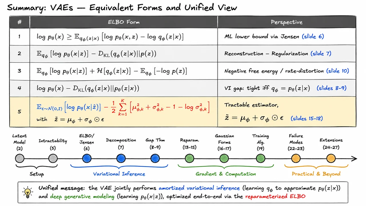
Before we can understand what a variational autoencoder is optimizing, we need to be precise about the problem it is trying to solve. A VAE is not merely an “autoencoder with noise.” It is a generative model: a model whose goal is to learn something about the probability distribution that produced the observed data.
Suppose we are given a dataset
where each observation . For images, might be the number of pixels; for audio, it might be waveform samples or spectrogram coefficients; for text embeddings, it might be the embedding dimension. The generative modeling problem is to learn a distribution that approximates the unknown data-generating distribution .
This goal has three closely related interpretations. First, we may want density estimation: given a new point , how likely is it under the model? That is, can we evaluate or approximate ? Second, we may want synthesis: can we draw new samples that look like plausible members of the dataset, but are not exact copies? Third, we may want representation learning: can the model discover compact, structured variables that explain meaningful factors of variation in the data?
These goals are connected, but they are not identical. A model may produce sharp-looking samples while assigning poor likelihoods, or it may achieve good likelihood while generating visually mediocre samples. VAEs are especially interesting because they try to tie these goals together through a probabilistic latent-variable framework: they define a likelihood, support sampling, and learn internal representations.
A first naive idea is to estimate the density directly from the observed data. For example, kernel density estimation places a small “bump” of probability mass around each training example:
In low dimensions, this can work surprisingly well. If the data points densely cover the relevant region of space, then nearby kernels overlap and form a smooth estimate of the distribution. But in high dimensions, this intuition breaks down catastrophically.
The reason is the curse of dimensionality. The volume of a ball of radius , or more generally the number of distinguishable regions in a -dimensional space, grows roughly exponentially with . For MNIST, a grayscale image lives in . Even images are vanishingly sparse in such a space. Almost every possible pixel vector is not a digit at all; it is visual noise. Worse, many distance-based intuitions fail: in very high dimensions, points tend to become nearly equidistant, making “nearest neighbors” and local smoothing much less reliable.
So the issue is not just that we need more data. The ambient space is overwhelmingly large, and the data occupies only a tiny, highly structured subset of it. A kernel density estimator spreads probability around observed examples in the ambient space, but most of that space is irrelevant. Unless the kernel bandwidth is extremely small, it assigns mass to unrealistic regions; if the bandwidth is extremely small, it assigns nearly zero density almost everywhere. Either way, the method fails to capture the actual structure of the data distribution.
This motivates the data manifold hypothesis. Although observations may be represented as vectors in a high-dimensional ambient space, the meaningful variation in the data often has much lower intrinsic dimension. For example, handwritten digits vary by stroke thickness, slant, rotation, identity, local style, and other factors. These factors are far fewer than 784 independent pixel degrees of freedom. Informally, the data may lie near a low-dimensional manifold embedded in the high-dimensional observation space.
This is where latent variables enter the story. Instead of modeling directly as an arbitrary point in the ambient space, we introduce a lower-dimensional variable
and imagine that observations are generated from these latent coordinates. The latent variable should capture the compact explanatory factors, while the model maps from latent space into data space. This does not mean the true data manifold is literally linear, smooth everywhere, or exactly -dimensional. Rather, it is a modeling assumption: useful data distributions often have enough low-dimensional structure that exploiting it is far better than treating all directions in equally.
The visual below condenses this motivation into a geometric picture. On the left, the high-dimensional ambient space is mostly empty: even many training examples provide negligible coverage when is large, which is why direct kernel-style density estimation becomes ineffective. On the right, the same data becomes much more intelligible when viewed as concentrated near a lower-dimensional manifold.
The key transition is from “estimate density everywhere in ” to “model how low-dimensional latent structure gives rise to high-dimensional observations.” That transition is the conceptual starting point for latent variable models, and it is exactly the path that will lead us to variational autoencoders.
The previous discussion framed generative modeling as a density-learning problem: we want a model that assigns high probability to realistic data and can also produce new samples. But high-dimensional observations—images, audio, text embeddings—rarely vary freely in all ambient dimensions. A handwritten digit image may have thousands of pixels, yet much of its variation can be described by a smaller set of factors: which digit it is, how thick the stroke is, whether it is tilted, how centered it is, and so on. Latent variable models make this intuition explicit.
The core assumption is that each observed data point is generated from an unobserved, lower-dimensional variable . We do not get to see in the dataset; it is a hidden explanation for the observation. Instead of modeling the distribution over directly, we define a two-step generative process:
Here, is a simple prior over latent codes, usually chosen to be a standard Gaussian. The conditional distribution is the decoder or generative model: given a latent code, it describes a distribution over possible observations. In modern VAEs, this conditional distribution is parameterized by a neural network , which maps latent coordinates into the parameters of a likelihood over data space.
This setup separates two kinds of complexity. The prior is deliberately simple: sampling from is easy, and its geometry is well behaved. The decoder carries the burden of learning how simple latent variation becomes rich observed structure. For example, in an idealized MNIST model, nearby values of might correspond to visually similar digits, while different directions in latent space could control properties such as digit identity, stroke width, or tilt.
The probability assigned to an observation is obtained by considering all possible latent explanations that could have generated it. This gives the marginal likelihood, also called the evidence:
This integral is the mathematical heart of latent variable modeling. It says: to evaluate how likely is, average the likelihood over every possible latent code , weighted by how plausible that code was under the prior. A particular might reconstruct very well, but if that lies in an extremely unlikely region of the prior, its contribution is limited. Conversely, common latent codes contribute more, but only if the decoder can plausibly produce from them.
This is why latent variable models are so appealing. They offer a structured way to generate data:
They also offer a conceptual interpretation of representation learning: the model is encouraged to organize meaningful variation in data through the latent space. If the learned representation is smooth, moving through -space should produce coherent changes in generated samples rather than abrupt jumps.
But the same integral that makes the model principled also creates the central computational difficulty. When is parameterized by a neural network, the integral
usually has no closed form. The decoder can be highly nonlinear, and the latent space may have many dimensions. Direct numerical integration becomes infeasible, and naïve Monte Carlo estimates can be too noisy or inefficient for maximum likelihood training. Therefore, although the model defines formally, we cannot usually evaluate or maximize directly.
This is the key tension that motivates variational inference and, ultimately, the VAE objective. We have a clean generative story and a meaningful likelihood, but the marginalization over hidden causes is intractable. The rest of the VAE framework can be understood as a way to optimize a tractable surrogate for this inaccessible log-likelihood.
The visual below compactly summarizes this idea. The left side uses a graphical-model view: a latent variable is drawn from the prior, then an observed variable is generated through , repeated independently across data points. The shaded observed node emphasizes that is in the dataset, while remains hidden.
The right side grounds the abstraction in an MNIST-style example: a latent code can be thought of as controlling semantic or stylistic factors that the decoder turns into an image. The important warning is the intractable integral over : even though the sampling story is simple, evaluating the probability of a given observation requires summing over all latent explanations, which is precisely what we cannot do directly with a neural decoder.
Having introduced latent variable models, we now run into the first serious computational obstacle: the model is easy to write down, but hard to fit. The whole appeal was to define a simple prior , pass through a decoder, and obtain a flexible distribution over observations . But maximum likelihood training asks us to evaluate
and that integral is exactly where the trouble begins. For simple decoders, the integral and the posterior over latents may be analytically tractable. For neural network decoders, they usually are not.
The classical tool for latent variable models is Expectation-Maximization. EM alternates between inferring the latent posterior under the current parameters and then updating the parameters using expectations under that posterior. The E-step requires
This equation is innocent-looking but deceptive. The denominator is the very marginal likelihood integral we were trying to avoid. In models with conjugacy or linear-Gaussian structure, the posterior has a known form and EM is elegant. But once the decoder becomes nonlinear, the posterior can become highly warped, multimodal, and unavailable in closed form.
A useful contrast is probabilistic PCA. Suppose
Because everything is linear and Gaussian, the posterior is also Gaussian. EM can compute its mean and covariance exactly. The latent space remains geometrically well-behaved: observing carves out an elliptical Gaussian belief over possible 's.
Now replace the linear map with a neural network :
The prior is still simple, and the observation noise may still be Gaussian, but the posterior is no longer Gaussian. The inverse image of a given observation under may contain many disconnected regions. Different latent codes can decode to similar observations. The posterior may have sharp ridges, separated modes, and strong nonlinear dependencies between latent dimensions. In other words, the generative direction may be easy to evaluate, while the inference direction is hard.
One tempting fallback is MAP inference: instead of representing the whole posterior, choose the most likely latent point,
This can be useful in some settings, but it is not a satisfactory replacement for posterior inference. A point estimate throws away uncertainty. If the posterior has several plausible modes, MAP picks one and ignores the rest. It also introduces an inner optimization problem for every datapoint, which is expensive during training. Worse, if we need gradients through that optimization procedure, the computation becomes cumbersome and brittle, especially when latent variables are discrete or when the optimization landscape is poorly conditioned.
Another seemingly generic solution is Monte Carlo EM. We might sample latent candidates from the prior,
and weight them according to how well they explain :
This is importance sampling with the prior as the proposal distribution. The problem is that the prior is usually a terrible proposal for the posterior. In high dimensions, most samples from land in regions that explain a specific extremely poorly. A tiny number of samples may receive almost all the probability mass, while the rest contribute essentially nothing.
This phenomenon is often called importance weight collapse. As the latent dimension grows, the effective number of useful samples can collapse toward one:
The phrase “effective sample size” is important: even if we draw thousands of samples, the estimator may behave as though it had only one meaningful sample. This creates exponentially high variance estimates of the E-step quantities and makes naive Monte Carlo learning impractical for expressive latent-variable models.
So the failure is not that EM, MAP, or Monte Carlo are conceptually wrong. Each is reasonable under the right assumptions. The failure is a mismatch between those assumptions and neural generative models:
The visual below compresses this comparison into the key geometric intuition. In the linear-Gaussian case, posterior inference is clean: the posterior over is a single Gaussian-shaped region, and EM can proceed exactly. In the nonlinear case, the posterior becomes irregular and multimodal, so the E-step no longer has a closed-form solution.
The weight-collapse sketch at the bottom emphasizes why simply sampling many 's from the prior does not rescue us. In high-dimensional latent spaces, almost all prior samples are irrelevant for a particular observation , and the importance weights concentrate on one lucky sample. This is the motivation for the next idea: instead of solving a separate hard inference problem from scratch for every datapoint, VAEs introduce amortized approximate inference—a learned encoder that predicts an approximate posterior directly.
The failure of direct EM or per-example MAP inference points us toward a different compromise: instead of solving a fresh optimization problem for every datapoint, we will learn a function that performs inference. This is the central move in a variational autoencoder. A VAE is not just “an autoencoder with noise”; it is a probabilistic latent-variable model equipped with a trainable approximation to the posterior.
The generative story begins with a latent variable , typically chosen to live in a relatively low-dimensional continuous space:
This distribution is called the prior. It says what kinds of latent codes are plausible before seeing any data. The standard Gaussian prior is not chosen because we believe the true hidden factors of images, text, or molecules are literally independent standard normal variables. Rather, it is chosen because it gives us a simple, smooth, sampleable reference distribution. Later, when we generate new data, we will sample and decode it into an observation.
The second ingredient is the decoder, also called the generative model or likelihood model. It specifies how an observed datapoint is produced from a latent code :
In a neural VAE, this conditional distribution is parameterized by a neural network . The network does not directly output “the reconstruction” in a purely deterministic sense; rather, it outputs the parameters of a probability distribution over possible observations. For continuous data, a common choice is an isotropic Gaussian likelihood,
where is the mean of the conditional distribution. For binary data, such as binarized MNIST pixels, a common choice is a Bernoulli likelihood,
Together, the prior and decoder define the actual generative model:
This joint distribution is the model’s claim about how data and latent variables co-occur. If we could compute the posterior exactly,
then inference would be straightforward: given an observed , infer which latent codes plausibly generated it. But the denominator,
is generally intractable for a nonlinear neural decoder. This is the same obstacle we encountered when trying to use exact EM: the posterior is the object we need, but it is not available in closed form.
The VAE introduces a third distribution to address this: the encoder, or approximate posterior,
Here another neural network, often denoted , maps an input datapoint to the parameters of a Gaussian distribution over latent codes:
This is an approximation to , not part of the generative model itself. The generative model is still . The encoder is an inference mechanism: it gives us a tractable distribution from which we can sample latent codes likely to explain .
The key innovation is amortized inference. In classical variational inference, we might introduce separate variational parameters for each datapoint, for example with its own . That would mean every new datapoint requires its own inference optimization. VAEs instead use a single shared network for all datapoints:
The cost of inference is therefore amortized over the dataset. We pay once to learn , and then inference for a new is just a forward pass. This is why VAEs scale well to large datasets and why they look architecturally like autoencoders: data goes through an encoder into a latent representation, then through a decoder back into data space. But probabilistically, the encoder and decoder play asymmetric roles.
There is also an important modeling assumption hidden in the standard encoder form. By choosing
we assume the approximate posterior is Gaussian with diagonal covariance. This makes sampling and KL-divergence computations convenient, but it can be restrictive. The true posterior may be multimodal, skewed, or highly correlated across latent dimensions. Much of the behavior of VAEs—including some failure modes we will discuss later—comes from the tension between a flexible neural decoder and a relatively simple approximate posterior family.
The three distributions therefore have distinct responsibilities:
The visual below consolidates this separation by showing two complementary paths. The generative path starts from and moves downward through to produce . The inference path goes in the opposite direction: given , the encoder produces a distribution over plausible latent codes.
The most important detail to keep in mind is that the right-hand path is not a separate model of the data. It is a learned approximation used to make training and inference tractable. The shared parameter vector is what makes the inference procedure amortized: instead of optimizing a new posterior approximation for every , the VAE learns one encoder network that serves the entire dataset.
Now that we have separated the VAE into its three distributions—the prior , the decoder , and the encoder-like approximation —we can ask the most basic statistical question: what objective should train the generative model? If the decoder is supposed to define a probability model over observations, then the natural answer is maximum likelihood. We want parameters that assign high probability to the observed dataset:
This is the same principle used in ordinary probabilistic modeling: choose the model under which the data would have been most likely. The complication is that in a latent-variable model, is not given directly. It is the probability of observing after averaging over all possible latent explanations .
For a single datapoint, the marginal likelihood, also called the evidence, is
so the log-evidence is
Conceptually, this integral says: sample a latent code from the prior, decode it into a distribution over , and average the probability assigned to the observed across all possible latent codes. If many plausible latent codes explain , the evidence should be high. If almost no latent code decodes near , the evidence should be low.
The problem is that this integral is almost never analytically tractable for a neural decoder. In a simple linear-Gaussian latent-variable model, the integral may have a closed form. But in a VAE, is parameterized by a deep network . The latent space is typically continuous, often , and the integrand can be nonzero over an enormous region. We are therefore trying to integrate a nonlinear neural-network-shaped function over a high-dimensional space:
There is no general symbolic simplification available.
A first instinct is to use Monte Carlo sampling from the prior. Draw
approximate the expectation, and then take the logarithm:
This looks reasonable, and for very large it is a consistent estimator. But as a training objective, it has two serious issues. First, prior samples are usually a terrible way to find the latent codes that explain a specific datapoint . In high dimensions, most will decode to samples unrelated to , so the average can be dominated by rare lucky samples. This leads to high variance.
Second, and more fundamentally, the log of a Monte Carlo average is a biased estimator of the log-evidence. The logarithm is concave, so Jensen’s inequality gives
The inequality is strict unless the random quantity inside the log is essentially constant. Equivalently, in the single-sample case,
This is the key obstruction: moving the logarithm outside or inside an expectation changes the objective. The log-evidence is what we want, but it contains an intractable integral. The expectation of the log-likelihood is tractable by sampling, but it is generally a lower quantity and, by itself, is not the right maximum-likelihood objective.
This is where the VAE’s central idea begins to emerge. We need a surrogate objective that is:
That surrogate will be the Evidence Lower Bound, or ELBO, written schematically as
The additional parameter appears because we introduce an inference network , whose role is to propose latent codes likely to explain the observed datapoint. Instead of sampling blindly from the prior, the VAE learns where in latent space to look.
The visual below compresses this motivation into three layers: the maximum-likelihood goal, the intractable log-evidence integral, and the failed naive Monte Carlo shortcut. The red warning around Jensen’s inequality highlights the precise mathematical reason we cannot simply replace the integral with a sampled average inside a logarithm and proceed as if nothing changed.
The bottom layer then points to the resolution: rather than estimating the log-evidence directly, we construct a computable lower bound with good gradient behavior. The next step is to derive that bound carefully and see exactly why it is lower, when it becomes tight, and how it decomposes into the reconstruction and KL terms used in VAE training.
Having written the evidence as an integral over the latent variable, we now face the central obstacle of latent-variable maximum likelihood: the quantity we want,
is usually not computable in closed form. The integral sums over all possible latent explanations of the observation . For expressive neural decoders , this marginalization is precisely what makes the model powerful — and precisely what makes direct optimization difficult.
The key variational idea is to introduce an auxiliary distribution , which we will later implement as the encoder. At this point, however, is just a mathematical device: a distribution over latent variables conditioned on the observed datapoint. We use it to rewrite the intractable integral as an expectation under a distribution from which we can sample.
Starting from the evidence,
we multiply and divide by :
This is an exact algebraic identity, not an approximation. It is the same logic as importance sampling: instead of integrating directly with respect to the latent variable measure, we express the integral as an expectation under a chosen proposal distribution :
There is an important support condition hidden in this step. The ratio must be well-defined wherever contributes mass. Informally, must not assign zero probability to latent regions that the model considers possible explanations of . Otherwise, the importance-weighted expression can become undefined or miss parts of the integral entirely.
Now comes the only inequality in the derivation. Since is concave, Jensen’s inequality tells us that for a positive random variable ,
Here the random variable is
Applying Jensen’s inequality gives
or equivalently,
This lower bound is the evidence lower bound, or ELBO:
The name is literal: it is a lower bound on the log-evidence . For any valid choice of ,
This is the foundational move in VAEs. We replace an intractable objective with a tractable lower bound that can be estimated by sampling from the encoder.
The bound becomes tight exactly when Jensen’s inequality becomes equality. For a concave function like , equality occurs when the random variable inside the expectation is constant almost surely under . In this case, we need
Rearranging,
So the ELBO is tight when the variational distribution exactly matches the true posterior . This is also why the encoder is often described as an approximate posterior: it is trained to behave like the posterior distribution that would make the bound exact, but which is usually unavailable because it depends on the intractable evidence .
This derivation matters because it gives us a practical optimization target with a clear interpretation:
There is a subtle but important caveat: maximizing a lower bound is not automatically the same as maximizing the original objective. If the bound is loose, we may improve without significantly improving . The success of VAEs depends on making the variational family expressive enough, and the optimization stable enough, that this lower bound remains a useful surrogate for maximum likelihood.
The visual below condenses the derivation into its three essential moves: start from the marginal likelihood, rewrite it as an expectation using , then apply Jensen’s inequality to move the logarithm inside the expectation. The boxed expression is the ELBO, the quantity we can optimize in place of the inaccessible log-evidence.
It also highlights the geometric meaning of the inequality: sits below , with a gap determined by how imperfect the variational posterior is. In the next section, we will decompose this same ELBO into the two terms that make VAEs operational: a reconstruction term and a KL regularization term.
Having obtained the ELBO through Jensen’s inequality, the next question is: what exactly are we optimizing? The expression
is already a valid lower bound on , but in this form it hides the two competing forces that make VAEs work. To understand the training objective operationally, we want to rewrite it in terms of the decoder likelihood and a penalty on the encoder distribution.
The key move is simply to expand the joint model. In a VAE, the generative story is assumed to factor as: first sample a latent variable from a prior , then sample the observation from a decoder likelihood . Therefore,
and taking logs gives
Substituting this into the ELBO gives
Because expectation is linear, we can separate the terms:
The first term has a direct modeling interpretation. We draw latent codes from the encoder distribution , then ask how much probability the decoder assigns back to the original observation . This is the reconstruction term:
It rewards latent representations that preserve information useful for explaining the input. If is a Bernoulli distribution, this often corresponds to a binary cross-entropy reconstruction objective; if it is a Gaussian with fixed variance, it becomes proportional to a negative squared-error loss. This is why VAEs often look, at implementation time, like autoencoders with a probabilistic reconstruction loss.
The second term is more subtle. Recall that the KL divergence is
Our ELBO contains the negative of this quantity:
So the ELBO decomposes into the now-famous form
This decomposition explains the central tension in VAE training. The reconstruction term wants to encode enough information about that the decoder can reconstruct it accurately. The KL term wants to stay close to the prior , usually a simple standard Gaussian such as . In other words, the encoder is not free to assign every datapoint an arbitrary isolated latent code; its codes must remain compatible with a shared latent space from which we can later sample.
This regularization is not merely aesthetic. Without it, the model could behave like an ordinary deterministic autoencoder: excellent reconstructions, but a latent space with holes, disconnected regions, and no reliable way to generate new samples by drawing . The KL penalty pushes the aggregate structure of the latent codes toward something smooth and sampleable. At the same time, if the KL pressure is too strong, the encoder may ignore , producing for every input. That failure mode is known as posterior collapse, and it causes the latent variable to carry little or no information.
A useful way to remember the objective is:
For the common Gaussian case, this tradeoff becomes especially convenient computationally. If
and
then the KL term has a closed-form expression. That means VAE training usually combines a Monte Carlo estimate of the reconstruction expectation with an analytic KL penalty, giving a stable and differentiable objective once we introduce the reparameterization trick.
The visual below condenses this derivation into its algebraic skeleton: start from the Jensen-derived ELBO, expand the joint distribution using the generative factorization, separate the expectation, and recognize the second piece as a negative KL divergence. The color split emphasizes that the final objective is not one monolithic loss, but a sum of two interpretable forces with opposite pressures.
Read the final boxed equation as the practical training objective for a single datapoint : maximize expected decoder log-likelihood while minimizing deviation from the prior. This compact decomposition is the bridge between the abstract variational bound and the loss function we will soon implement in an actual VAE.
Having split the ELBO into a reconstruction term and a KL-to-prior regularizer, we can now ask a deeper question: what exactly did we lose when we replaced the true log-evidence by the ELBO? The answer is one of the most important identities in variational inference: the missing quantity is not mysterious approximation error, nor a loose heuristic penalty. It is exactly a KL divergence between the variational encoder and the true Bayesian posterior.
For a latent-variable model, the evidence is
and the true posterior over latents is
This posterior is the distribution we would ideally use for inference: after observing , it tells us which latent explanations are plausible. The difficulty is that depends on , the very integral we cannot usually compute. VAEs therefore introduce an encoder , a tractable approximation to this intractable posterior.
The central theorem says that, for a suitable variational distribution ,
Here the ELBO is
So the ELBO is not merely inspired by the evidence. It is the evidence minus a very specific nonnegative gap.
Because KL divergence is always nonnegative,
we immediately recover the lower-bound property:
This also explains the name Evidence Lower Bound. The ELBO sits below the log-evidence, and the vertical distance between them is precisely the mismatch between the approximate posterior and the true posterior .
The theorem also tells us exactly when the bound is tight. We have
if and only if
In words: the ELBO becomes the true log-evidence exactly when the encoder recovers the true posterior. There is no remaining variational gap. This is why the encoder is not just an auxiliary neural network used for amortized sampling; it is performing approximate Bayesian inference.
There is a subtle support assumption hiding here. For the KL
to be finite, should not place probability mass where the true posterior has zero mass. More formally, we usually require to be absolutely continuous with respect to . At the same time, if the variational family is too restrictive and cannot represent the true posterior’s important regions, the gap cannot close. This is one reason why posterior approximation quality depends not only on optimization, but also on the expressiveness of the encoder family.
The identity has an important optimization consequence. Suppose is fixed. Then is constant with respect to , so maximizing the ELBO over is exactly equivalent to minimizing
That is the variational inference interpretation of the VAE encoder: training by maximizing the ELBO pushes it toward the true posterior. When we also optimize , we are doing two things at once: learning a generative model that assigns high probability to the data, and learning an approximate inference model that explains each datapoint in latent space.
A useful way to remember the theorem is:
The visual below compresses this relationship into a geometric picture. The log-evidence is represented as a fixed point on a “nats” axis, while the ELBO lies to its left. The red interval between them is the posterior KL divergence. If the encoder improves, that interval shrinks; if matches , the two points coincide.
The three corollaries in the visual are therefore not separate facts, but direct consequences of the same decomposition: the ELBO is a lower bound because KL is nonnegative; it is tight exactly when the approximate and true posteriors agree; and maximizing it with respect to is variational inference. The next step is to prove the identity algebraically, showing how Bayes’ rule turns the apparently inaccessible evidence into the sum of an optimizable lower bound and an explicit posterior mismatch term.
Having stated that the gap between the log evidence and the ELBO is a KL divergence, we should now verify that this is not a heuristic slogan. It is an exact identity. The derivation is short, but it is worth reading carefully because it explains why variational inference works: we are not inventing an arbitrary surrogate objective; we are decomposing the true marginal log-likelihood into a tractable lower bound plus a nonnegative error term.
Fix one observed datapoint . The model defines a latent-variable joint distribution
and the true posterior is
The problem is that , the evidence, usually requires integrating out :
In a VAE, this integral is generally intractable because the decoder is represented by a neural network. So instead of working directly with the true posterior , we introduce an approximate posterior, or encoder distribution,
The key question is: how does optimizing an objective involving relate to maximizing the true log evidence ?
Start from the KL divergence between the variational posterior and the true posterior:
Now substitute Bayes’ rule into the true posterior term:
Taking logs gives
Therefore,
The subtle but crucial observation is that does not depend on . The expectation is over , while is fixed. So we can pull outside the expectation:
Equivalently,
The expectation inside the negative sign is precisely the evidence lower bound:
So the KL divergence becomes
Rearranging gives the central decomposition:
This is the whole proof. No approximation has been made. We used only the definition of KL divergence, Bayes’ theorem, and the fact that constants can be moved outside expectations.
The consequence is immediate. Since KL divergence is always nonnegative,
we have
That is why is called a lower bound on the log evidence. The bound is tight exactly when
which occurs when
almost everywhere under . In words: the ELBO equals the true log evidence when the encoder distribution exactly matches the model’s true posterior.
This identity also clarifies a common failure mode in variational modeling. Maximizing the ELBO improves a lower bound on , but it does so through the restricted family . If the encoder family is too limited, the KL gap may remain large even after optimization. The objective is still valid, but the approximation may be poor. Conversely, if is expressive enough and optimization succeeds, the ELBO can become a very accurate proxy for the true marginal likelihood.
The visual below compresses the derivation into a chain of equalities: start with the KL divergence to the true posterior, replace the posterior using Bayes’ theorem, separate the constant , recognize the ELBO, and rearrange. The boxed final identity is not an additional assumption; it is simply the same expression written so that the evidence appears on the left.
It is useful to keep this picture in mind as we move forward. The ELBO is not merely “reconstruction plus regularization” yet—that interpretation will come after expanding the joint model. At this stage, the most important fact is structural: log evidence decomposes exactly into an optimizable lower bound plus a nonnegative posterior-approximation gap.
Having just seen that the ELBO differs from the true log evidence by a nonnegative KL gap, we can now reinterpret the bound in a more operational way. The ELBO is not merely an algebraic trick for lower-bounding ; it is the objective that tells a VAE how to trade off using latent information against staying compatible with the prior.
For a single datapoint , the VAE objective is
The first term is the reconstruction term. It asks: if the encoder distribution samples a latent code , how much probability does the decoder assign back to the original observation ? Maximizing this term encourages the latent representation to preserve information that the decoder needs. In an image VAE, this means encoding shape, pose, color, texture, or any features that help predict the input under the chosen likelihood model.
The second term is the regularization term, but that phrase can be slightly misleading if we think of it as a generic penalty. More precisely, it penalizes the encoder distribution for moving too far away from the prior , usually . This matters because generation will later sample , not . If the encoder learns latent codes that live in strange isolated regions far from the prior, then samples drawn from the prior may decode poorly. The KL term forces the aggregate geometry of the latent space to remain usable for generation.
We can unpack the KL penalty further using
Therefore,
This decomposition reveals two forces hidden inside the regularization term. The entropy term rewards the encoder for being uncertain, or spread out, rather than collapsing to a deterministic point code. Meanwhile, the expected negative log prior term penalizes codes that fall in regions where assigns low probability. For a standard Gaussian prior, this means the model is discouraged from placing latent mass far away from the origin.
So the ELBO is balancing two competing desires:
This tension is fundamental. If the KL penalty is too weak, the encoder may memorize examples using highly specialized latent codes, producing good reconstructions but a poorly organized latent space. If the KL penalty is too strong, the encoder may ignore and make , which can lead to posterior collapse: the decoder receives little useful information from , and the latent variables stop carrying semantic structure.
This is why the ELBO also has a natural rate–distortion interpretation. The KL term acts like a rate: it measures how many nats, or bits up to a constant conversion, are required to encode using a distribution different from the prior. The reconstruction error acts like a distortion: poor reconstructions correspond to high distortion, while high log-likelihood corresponds to low distortion. Maximizing the ELBO means finding a good operating point between compression cost and reconstruction fidelity.
The connection to physics and variational inference comes from writing the training problem as minimization of the negative ELBO:
This quantity is often called the variational free energy or negative evidence lower bound. Since we previously established
minimizing free energy simultaneously pushes the ELBO upward and tries to reduce the gap between the approximate posterior and the true posterior . The bound becomes tight exactly when
assuming the variational family is expressive enough to represent the true posterior.
The visual below condenses this interpretation into a balance: reconstruction pulls the objective toward faithful recovery of , while KL regularization pulls the encoder distribution back toward the prior. The scale metaphor is useful because neither side is “bad”; a good VAE needs both. Reconstruction gives the latent variable meaning, while the KL term gives the latent space global structure.
It also highlights the rate–distortion view: moving toward lower distortion usually requires spending more rate, while enforcing a very low rate often sacrifices detail. Much of practical VAE design—choosing decoder likelihoods, KL schedules, -VAE objectives, or more expressive priors—is about controlling exactly where this operating point lies.
Having seen the ELBO as a negative free energy, it is worth pausing on a case where nothing is hidden behind approximation. In most VAE settings, the posterior is intractable, which is exactly why we introduce a variational distribution . But in a one-dimensional linear-Gaussian model, the posterior, marginal likelihood, KL terms, and ELBO can all be written down exactly. That makes it a useful sanity check: if our interpretation of the ELBO is right, then optimizing it over a sufficiently expressive variational family should recover the true posterior and make the ELBO equal to the evidence.
Consider the toy generative model
Here the latent variable is drawn from a standard normal prior, and the observation is a noisy version of with small Gaussian noise variance . Because both the prior and likelihood are Gaussian, the marginal distribution of is also Gaussian:
so the log evidence is available in closed form:
The true posterior is also Gaussian. Combining the prior precision with the likelihood precision , the posterior variance is
and the posterior mean is the precision-weighted estimate
Thus
This already contains an important intuition. The observation pulls the posterior mean toward , but not all the way: the prior still shrinks the estimate toward zero. Since the observation noise is small, the posterior variance is much smaller than the prior variance. For , we get
Now suppose our variational family is
This family is expressive enough to contain the true posterior exactly, because the true posterior is also a one-dimensional Gaussian. The ELBO is
In this Gaussian case, both terms can be evaluated analytically. The expected reconstruction term is
because under ,
The KL regularizer against the standard normal prior is
So the ELBO is a deterministic function of only two variational parameters, and . There is no Monte Carlo noise, no neural network approximation, and no optimization mystery. We can inspect the entire objective surface directly.
The key identity from the previous section was
Because the evidence does not depend on , maximizing the ELBO over is equivalent to minimizing
In this toy example, the minimum possible KL gap is exactly zero, since the variational family contains the true posterior. Therefore the global maximizer is
or equivalently,
At that point,
and the ELBO becomes tight:
This is the tightness corollary in its cleanest possible form.
It is useful to compare three operating points for :
The visual below consolidates these facts in two complementary ways. The contour plot treats the ELBO as a surface over : the maximum occurs exactly at the true posterior parameters, not merely near them. The prior-like approximation sits far away from the optimum, while the centered-but-wide approximation lands on the correct mean but remains suboptimal because its uncertainty is wrong.
The companion bar chart emphasizes the decomposition
For each candidate , the ELBO plus the KL gap reaches the same evidence level. In the exact posterior case, the red “gap” disappears entirely, making the lower bound not just a bound, but the true log marginal likelihood.
The one-dimensional Gaussian example makes the ELBO feel almost deceptively friendly: the KL term can be written down, the expectation can sometimes be evaluated or estimated, and the whole objective looks like something we should be able to optimize with ordinary backpropagation. But the moment we replace that toy setup with a neural encoder and decoder, a subtle obstruction appears. The problem is not that the ELBO is undefined, nor that Monte Carlo estimation is impossible. The problem is that the Monte Carlo samples themselves sit in the middle of the computation graph.
Recall that for a single datapoint , the VAE objective is
When we differentiate with respect to the encoder parameters , the gradient decomposes as
The KL term is usually not the source of trouble in the standard VAE. If is a diagonal Gaussian,
and the prior is , then the KL divergence has a closed form. It is just a differentiable expression involving and . Autodiff can handle this directly.
The reconstruction term is different because the distribution inside the expectation depends on :
Here controls where we sample from. Changing changes the density , which changes the regions of latent space that contribute to the expectation. This is not the same as differentiating an ordinary deterministic function. The parameter affects the objective through the sampling distribution itself.
A natural first attempt is to use Monte Carlo sampling. Draw
and approximate the reconstruction expectation by
This gives an unbiased estimate of the expectation. For optimizing , it is fine: once is sampled, the decoder likelihood is an ordinary differentiable function of . But for optimizing , naive backpropagation runs into a wall. The sampled value is not represented as a differentiable deterministic function of . In the computation graph, the operation “sample from ” behaves like a stochastic node, not like a smooth layer.
This is the key failure mode of naive Monte Carlo:
does not correctly estimate
If we treat the sampled values as fixed constants after sampling, then the reconstruction term has no differentiable path back to . Informally, the gradient is blocked at the sampling operation. More precisely, the particular sampled numerical value may change if we rerun the sampler with a different , but that dependence is not available to standard backpropagation as a local derivative through the realized sample.
There is a general-purpose workaround called the score-function estimator, often known in this context as REINFORCE. It uses the identity
This identity is valid under mild regularity assumptions and does not require differentiating through the sampled value . Instead, it differentiates the log-density of the sampling distribution. That is powerful: it works even for discrete random variables, where ordinary pathwise derivatives are unavailable.
But for VAEs with neural decoders, this estimator is usually too noisy to be practical without substantial variance reduction. The scalar reward-like term can vary dramatically across samples, especially early in training. Multiplying it by often produces gradients with very high variance. In principle the estimator is unbiased; in practice, its updates can be so unstable that learning becomes slow, erratic, or ineffective.
So the issue is not merely “sampling is random.” The deeper issue is that we need a low-variance differentiable estimator of how the reconstruction objective changes when the encoder distribution changes. Naive Monte Carlo gives samples but no usable pathwise gradient. REINFORCE gives a gradient but often with prohibitive variance. This tension is exactly what motivates the reparameterization trick.
The visual below compresses this obstruction into a computation graph. The forward pass is straightforward: is encoded into parameters of , a latent sample is drawn, and the decoder evaluates . The backward pass is where the asymmetry appears: gradients flow cleanly through the decoder, but the attempted gradient path back through the stochastic sampling node is blocked.
The small REINFORCE annotation is the important caveat. There is a mathematical gradient estimator that avoids differentiating through the sample, but it pays for that generality with high variance. The next step is to replace the problematic sampling operation with an equivalent differentiable construction—one that preserves the same distribution over , while allowing backpropagation to reach .
The obstruction we just ran into was not that the encoder distribution is mysterious, nor that Gaussian sampling is impossible to differentiate in some philosophical sense. The issue is more specific: if we treat the operation “draw ” as an opaque stochastic node, then the sampled value changes with only through the distribution from which it was drawn. Standard backpropagation expects deterministic computational paths; it does not know how to assign a pathwise derivative through the act of sampling itself.
The reparameterization trick resolves this by changing how we generate the same random variable. Instead of sampling directly from a -dependent Gaussian, we sample from a fixed, parameter-free source of randomness and then transform that noise deterministically using the encoder outputs. For the diagonal Gaussian encoder used in the standard VAE,
we write a sample as
This is the core identity. The randomness now lives entirely in , whose distribution does not depend on . The encoder parameters only determine the deterministic map that takes to .
It is worth verifying that this has not changed the distribution being sampled. Componentwise,
An affine transformation of a standard normal random variable is normal, with shifted mean and rescaled variance:
Since the are independent under , the resulting vector has diagonal covariance:
So the reparameterized sample is distributionally identical to a direct sample from the encoder. The trick is not an approximation to the Gaussian; it is an exact change of representation.
The important shift is computational. Before reparameterization, we had a sample , and the dependence of on was hidden inside the sampling operation. After reparameterization, we have
where is treated as an external random input. For a fixed draw of , the map from to is just an ordinary differentiable computation graph. Gradients can flow through , through , and then through the decoder likelihood term .
This is why the reparameterization trick is sometimes called a pathwise gradient estimator. Instead of asking how the probability density changes with , we ask how the sampled point moves in latent space when changes while holding the underlying noise fixed. Intuitively, chooses a location in “standard normal coordinates,” and the encoder stretches and shifts that location into the latent space used by the decoder.
For example, if increasing one encoder parameter increases , then every sampled shifts upward by the corresponding amount. If increasing another parameter increases , then samples with positive move upward and samples with negative move downward. These are ordinary derivatives:
Backpropagation can now see exactly how changing the encoder changes the latent sample and, through the decoder, changes the reconstruction term in the ELBO.
There are a few assumptions hiding here. First, we need a distribution that can be expressed as a deterministic transformation of parameter-free noise. This is easy for location-scale families such as Gaussians, where samples can be written as “mean plus scale times noise.” Second, the transformation should be differentiable with respect to the parameters we want to optimize. Third, the base noise distribution must not depend on ; otherwise the original problem reappears inside the supposedly fixed randomness.
In its most general form, the idea is
where is fixed and is differentiable. The diagonal Gaussian VAE is the canonical example, but the principle extends beyond it whenever such a transformation is available. When it is not available—for example, for many discrete latent variables—we need different gradient estimators or relaxations, and those usually come with higher variance or bias.
The visual below compresses this logic into two computation graphs. The left side represents the problematic formulation: determines a distribution, a stochastic sample is drawn, and the gradient path is interrupted at that sampling node. The right side rewrites the same sample as a deterministic function of encoder outputs and independent noise. The stochasticity has not disappeared; it has simply been moved to a place where it no longer carries -dependence.
The key message to carry forward is that reparameterization does not make the VAE deterministic. Each forward pass can still use a fresh , so the latent code remains random. What changes is that, conditional on that noise draw, the ELBO becomes an ordinary differentiable objective with respect to . That is the bridge from stochastic latent-variable learning to standard neural-network optimization.
Having rewritten sampling as , the next question is not merely whether this is a convenient implementation trick. The real question is whether it gives us the right gradient. If we replace a draw from with a deterministic transformation of noise, are we still estimating
without bias?
This matters because the VAE objective contains expectations over latent variables sampled from the encoder distribution. For a single datapoint , the reconstruction-related part of the ELBO often has the form
where, for example, may be . The encoder parameters affect this expectation indirectly: changing changes the distribution over . Naively sampling creates a problem for backpropagation because the sampling operation itself is not a deterministic differentiable map of .
The reparameterization trick resolves this by expressing the random variable as
Now all randomness lives in , whose distribution does not depend on . The dependence on has been moved into a deterministic function:
So instead of differentiating through the act of sampling from , we differentiate through the deterministic path
The theorem states that, under the usual smoothness and integrability assumptions that allow us to interchange differentiation and expectation,
This is the central identity. The left side is the gradient we actually want: the derivative of an expectation under the encoder distribution. The right side is something we can estimate by ordinary backpropagation after sampling . Importantly, the expectation is now over , a fixed distribution independent of .
Given independent samples , the Monte Carlo estimator is
Because each term inside the average is an unbiased draw from the expectation on the right-hand side of the theorem, linearity of expectation gives
So the estimator is unbiased: averaging over repeated draws of , it recovers the exact gradient of the expected objective.
There are a few assumptions hiding inside this clean statement. First, must be differentiable with respect to , and the transformation from to must also be differentiable. This is why the standard Gaussian VAE encoder, parameterized by and , is so convenient. Second, the support of the distribution should not change in a pathological way as changes; otherwise, differentiating under the integral can become delicate. Third, the estimator is unbiased for the gradient of the reparameterized expectation, but finite-sample estimates still have variance. Unbiased does not mean noiseless.
The reason this estimator is so effective is not only that it is unbiased, but that it tends to have low variance. Compare it to the score-function or REINFORCE estimator:
REINFORCE is also unbiased and applies more generally, including to discrete random variables. But it usually has much higher variance because it does not exploit the local derivative . It treats more like a black-box reward. The reparameterized estimator, by contrast, uses the geometry of : gradients flow through the sampled latent value back into and .
This explains a practical fact about VAEs: we often use latent sample per datapoint during training. At first this may seem surprisingly crude, but minibatch stochastic optimization already averages gradients across many datapoints. The total gradient noise comes from both minibatch sampling and latent-variable sampling; in practice, the low variance of the pathwise gradient makes a single latent draw per example sufficient for stable learning.
The visual below condenses this theorem into two linked ideas. The top part emphasizes the algebraic identity: a gradient of an expectation under can be rewritten as an expectation over fixed noise , with gradients traveling through the deterministic map . The key annotation is that is independent of , which is precisely what makes ordinary backpropagation valid.
The bottom part gives the statistical intuition. Both REINFORCE and the reparameterized estimator are centered on the true gradient, so both are unbiased. But the REINFORCE distribution is much wider, representing high-variance gradient estimates, while the reparameterized estimator concentrates much more tightly around the true value. That difference in variance is what turns the theorem from a formal identity into a practical training method for VAEs.
Now that we know the reparameterized gradient estimator is unbiased, it is worth slowing down and asking why the identity is true. The key point is not mysterious: we are simply rewriting a -dependent distribution as a deterministic transformation of noise drawn from a fixed distribution. Once the randomness no longer depends on , differentiation becomes an ordinary backpropagation problem through a deterministic computation graph.
Start with the quantity we care about. For a fixed datapoint , suppose the encoder distribution is a diagonal Gaussian,
and suppose is some downstream scalar objective term, such as a decoder log-likelihood contribution. We want the gradient
The difficulty is that the distribution inside the expectation depends on . If we sample , the sample itself changes as the encoder parameters change, but this dependence is not explicit in the notation. Naively differentiating through a random draw is not well-defined in the usual computational graph sense.
Writing the expectation as an integral makes the dependency explicit:
Here, appears in the density . A score-function estimator would differentiate the density directly, producing terms involving . That approach is general, but often high-variance. The reparameterization trick instead asks whether we can move the -dependence out of the density and into the argument of .
For a diagonal Gaussian, we can. Let
and define
This deterministic transformation maps standard normal noise into a sample from . Componentwise,
Assuming , this map is invertible in each coordinate:
The Jacobian is diagonal, with entries , so the volume element transforms as
This is the whole mathematical engine of the proof. Under the change of variables , the original density-weighted measure becomes
Therefore,
Equivalently,
Notice what changed. The distribution is now fixed: it does not depend on . All dependence on has moved into the deterministic map
That is why backpropagation becomes possible. We are no longer differentiating “through sampling” from a moving distribution; we are differentiating through a deterministic function of fixed external noise.
Under the usual regularity assumptions—smooth enough , differentiable encoder outputs, and an integrable dominating function allowing us to exchange differentiation and integration—we can pass the gradient through the expectation:
Combining the equality of expectations with this differentiation step gives the reparameterized gradient identity:
This is exactly the statement that the Monte Carlo estimator
is unbiased for the desired gradient.
There are two subtle assumptions hiding here. First, the transformation must be valid: for the diagonal Gaussian case, this means the scale parameters are positive and the mapping between and is invertible almost everywhere. In practice, VAEs often parameterize or use a softplus transformation to guarantee positivity. Second, exchanging and the integral requires mild analytic conditions. Neural networks used in practice are usually treated as satisfying these conditions almost everywhere, but this step is still a mathematical assumption, not magic.
The practical takeaway is compact:
The visual summary below condenses the proof into its four logical moves: write the expectation as an integral, perform the Gaussian change of variables, observe that the transformed density becomes , and finally move the gradient through the expectation because is independent of .
The highlighted substitution is the pivotal step. Once has been rewritten as , the proof is essentially finished: the parameter dependence has migrated from the probability measure into a differentiable deterministic path, which is precisely what makes the VAE encoder trainable with low-variance gradient estimates.
Now that we have a pathwise gradient estimator for samples from the encoder, it is tempting to think that every part of the VAE objective needs Monte Carlo estimation. But one of the conveniences of the standard VAE is that this is not true. The reconstruction term usually requires samples , because it passes through a nonlinear decoder. The KL regularizer, however, has a closed-form expression when the encoder is Gaussian and the prior is standard normal.
Recall the per-example ELBO:
In the common diagonal Gaussian VAE, the encoder outputs two vectors:
and defines
The prior is usually chosen as
This particular pairing is not accidental. A diagonal Gaussian compared against a standard Gaussian gives a KL term that decomposes dimension-by-dimension. That means the model can penalize each latent coordinate independently for moving its posterior mean away from , or its posterior variance away from .
Start from the definition:
Because both distributions factorize across latent dimensions, their log-densities are sums over coordinates. Suppressing constants that will cancel or collect into dimension-independent terms, we can write
Here and mean the -th encoder outputs for the current datapoint . The expectation is still with respect to , but now only simple Gaussian moments are needed. Under ,
Substituting these moments and simplifying gives the exact closed form:
This expression is worth reading term by term. The penalty discourages the approximate posterior from shifting its mean far away from the prior mean . The combination
penalizes the posterior variance for deviating from the prior variance . It is minimized at , where it equals . Thus each latent coordinate pays no KL cost only when
meaning matches the prior along that coordinate.
A crucial practical point is that this KL term is fully differentiable and sampling-free. We do not need to draw to estimate it, and we do not need the reparameterization trick for this part of the objective. Gradients can flow directly through the encoder outputs and , or more commonly through and , since neural networks typically output log-variance for numerical stability.
This exactness also clarifies an important failure mode. Because the KL term pushes toward , a powerful decoder may learn to reconstruct well while ignoring . In that case the encoder can choose and , making the KL nearly zero. This is one view of posterior collapse: the approximate posterior becomes almost identical to the prior, so the latent code carries little information about .
There are a few assumptions hiding inside the neat formula:
The visual below condenses the derivation into the three essential moves: expand the KL definition, substitute the diagonal Gaussian log-densities, and apply the two Gaussian moment identities. The boxed expression is the quantity that appears directly in a VAE implementation.
It also separates the computational roles of the two ELBO terms. The KL side is analytic and deterministic; the reconstruction side still requires samples from , which is where the reparameterization trick from the previous section becomes necessary.
Having handled the KL term for a Gaussian encoder, the remaining piece of the ELBO is the part that asks a simple but crucial question: if we sample a latent code from the encoder, how well can the decoder explain the original observation? This is the reconstruction term,
It is often implemented as a mean-squared error loss, but that is not merely a convenient engineering choice. Under a Gaussian decoder assumption, MSE falls directly out of the likelihood model.
Assume the decoder defines a conditional Gaussian distribution over observations:
Here is the decoder network output, interpreted as the mean of the conditional distribution over . The variance says that, given , each observed dimension is corrupted by independent isotropic Gaussian noise with the same variance . This is a modeling assumption: it is reasonable for continuous-valued data after suitable normalization, but it is not automatically appropriate for binary pixels, counts, categorical variables, or perceptually structured image data.
For one latent sample , the Gaussian log-likelihood is
where is the dimensionality of . The first term is the Gaussian normalization constant. If is fixed, it does not depend on the decoder parameters . The second term is the squared reconstruction error, scaled by . Therefore, maximizing the Gaussian likelihood pushes toward in squared-error distance.
Inside the VAE, however, is not a single deterministic code. It is drawn from the approximate posterior , so the ELBO uses the expected log-likelihood:
Using the reparameterization trick, we usually write the sampled latent variable as
so the reconstruction term becomes an expectation over noise injected through a differentiable transformation. This is what lets gradients flow not only into the decoder parameters , but also back into the encoder parameters .
If is treated as a fixed hyperparameter, then maximizing the reconstruction term with respect to is equivalent to minimizing
up to a constant and a positive scaling factor. This is the precise sense in which the Gaussian decoder gives rise to expected MSE as the reconstruction loss. In practice, this expectation is usually approximated with one or a few Monte Carlo samples of per datapoint.
There are two subtle points worth keeping separate. First, the constant term
can be dropped only when is fixed. If is learned, that term matters; otherwise the model could change its variance without paying the correct likelihood normalization cost. Second, although dropping constants is harmless for optimizing , the reconstruction expectation still depends on through . So the encoder is trained not only to match the prior through the KL term, but also to choose latent distributions that allow accurate reconstructions.
The variance also has an important practical interpretation. In the full ELBO,
the reconstruction penalty is scaled by . Smaller makes reconstruction errors more expensive relative to the KL regularizer; larger softens the reconstruction pressure and makes the KL term comparatively more influential. Thus acts like a reconstruction–regularization trade-off knob, much like the weighting coefficient in a -VAE, though it arises from the likelihood model itself.
This likelihood choice also helps explain a classic VAE failure mode: blurry reconstructions. A Gaussian decoder trained with squared error is rewarded for predicting conditional means. When the posterior or decoder is uncertain among several plausible outputs, averaging them can produce visually smooth or blurry samples. This is not just an optimization artifact; it is partly a consequence of the assumed observation model. For binary data, a more appropriate decoder is often Bernoulli,
which leads to a binary cross-entropy reconstruction term rather than MSE.
The visual below condenses this derivation into a chain: start from the Gaussian decoder, expand the log-likelihood, take the expectation under the encoder distribution, and then drop the -constant terms to reveal the expected MSE objective. The key algebraic move is that the squared Euclidean error appears directly inside the Gaussian log-density.
It also highlights the modeling choices surrounding the derivation: the reparameterized sample is what makes the expected reconstruction loss trainable by backpropagation, the Bernoulli alternative reminds us that MSE is not universal, and the note about previews how the reconstruction term will be balanced against the KL divergence in the full VAE objective.
Now that the Gaussian decoder has turned the reconstruction term into something as familiar as squared error, we can finally assemble the pieces into the objective that is actually optimized in a VAE. The important point is that the VAE loss is not just reconstruction error with noise injected into the latent space. It is a variational lower bound with two coupled responsibilities: explain each datapoint well through the decoder, while keeping the encoder’s approximate posterior close enough to the prior that generation remains possible.
For a single datapoint , the ELBO is
The first term rewards latent samples that allow the decoder to assign high probability to the observed datapoint. The second term penalizes the encoder distribution for drifting too far from the prior , usually . This is what makes the latent space usable at generation time: after training, we want to sample , not from some fragmented collection of unrelated encoder distributions.
In practice, the expectation in the reconstruction term is estimated with samples. With the reparameterization trick, we write
This separates the randomness from the encoder parameters . Instead of sampling from a distribution whose parameters depend on in a way that blocks ordinary backpropagation, we sample parameter-free noise and transform it differentiably. That is the key technical move that allows gradients from the decoder’s reconstruction likelihood to flow backward through , then into and .
Using one Monte Carlo sample , the per-datapoint stochastic ELBO estimate becomes
Here the KL term has been written in closed form for the common diagonal Gaussian encoder
with standard normal prior . This analytic KL is one of the conveniences of the classical VAE setup. It avoids adding more sampling noise to the objective and gives a direct regularizing signal to the encoder.
A useful way to read the objective is as a controlled compromise:
This compromise is also where many VAE failure modes originate. If the KL penalty dominates too early, the encoder may learn for all , causing posterior collapse: the latent variable carries little information, and the decoder behaves almost like an unconditional model. If the reconstruction term dominates, the model may encode datapoints very precisely but produce a latent space that does not match the prior, making prior samples poor. With Gaussian decoders, another common issue is blurry reconstructions, because maximizing a pixelwise Gaussian likelihood often encourages conditional means rather than sharp, multimodal outputs.
For a dataset , training maximizes the sum of per-datapoint estimates:
Since full-dataset optimization is usually impractical, we use minibatches. For a batch of size , an unbiased estimate of the full objective is
Many implementations omit the factor when optimizing an average loss, because it only rescales the gradient for a fixed dataset and can be absorbed into the learning rate. What matters conceptually is that the minibatch objective estimates the same dataset-level ELBO. Also note the sign convention: derivations usually maximize the ELBO, while code often minimizes the negative ELBO, sometimes reported as reconstruction loss plus KL penalty.
The gradient dependencies are asymmetric but tightly coordinated. The decoder parameters appear only inside the likelihood term , so is ordinary decoder backpropagation. The encoder parameters , however, receive two kinds of signal: an analytic KL gradient that pushes toward zero and toward one, and a reconstruction gradient that flows through the reparameterized latent sample . This is why the full VAE objective trains encoder and decoder jointly rather than treating inference and generation as separate procedures.
The visual below condenses this entire training objective into its two main colored pathways. The blue reconstruction path represents the stochastic, reparameterized route from encoder outputs through into the decoder likelihood. The red KL path represents the closed-form regularizer acting directly on the encoder’s Gaussian parameters.
It also separates the three levels at which the same idea appears: the per-datapoint ELBO estimate, the full-dataset sum, and the minibatch estimator used in SGD. That hierarchy is worth keeping in mind before moving to the training algorithm: implementation is mostly bookkeeping, but the bookkeeping must preserve these two terms and their gradient paths.
Now that the ELBO has been assembled into a reconstruction term minus a regularization term, the remaining question is operational: what exactly happens during one training iteration? A VAE can look conceptually complicated because it contains an encoder, a decoder, a latent random variable, and a variational objective. But the actual training loop is quite close to ordinary minibatch SGD once we express the stochastic latent sample in a differentiable way.
For each datapoint in a minibatch, the encoder produces the parameters of an approximate posterior distribution,
The diagonal Gaussian assumption is doing a lot of work here. It makes sampling cheap, makes the KL divergence against the standard normal prior analytic, and gives us a simple parameterization for uncertainty in each latent dimension. In implementations, the network often predicts , or logvar, rather than directly, because the variance must remain positive and because log-variance is numerically more stable.
The central step is the reparameterized forward pass. Instead of sampling directly from , we sample parameter-free noise
and construct
This turns the random draw into a deterministic differentiable function of , , and external noise . That distinction is essential: gradients cannot flow through “sample from this distribution” in the usual backpropagation sense, but they can flow through addition, multiplication, and neural network outputs. The randomness remains, but it has been isolated from the parameters.
Once is sampled, the decoder evaluates the likelihood of reconstructing from that latent code:
This term depends on the chosen observation model. For binarized MNIST, it is usually a Bernoulli log-likelihood. For continuous data, one often uses a Gaussian likelihood, sometimes with fixed variance. This modeling choice matters: a simple Gaussian decoder trained with squared-error-like losses often encourages averaged reconstructions, which is one reason VAEs can produce blurry samples compared with adversarial models.
The KL term is computed analytically for each example because both and the prior are Gaussian. For a -dimensional diagonal posterior,
This term penalizes approximate posteriors that drift too far from the prior. Intuitively, it asks the encoder to use latent space economically: encode information only when it improves reconstruction enough to justify the cost. That tradeoff is powerful, but it also creates one of the most important VAE failure modes: posterior collapse. If the decoder is expressive enough to model the data without using , optimization may drive close to , making the latent code nearly uninformative.
Putting the two pieces together, a single-sample Monte Carlo estimate of the per-example ELBO is
Using one latent sample per datapoint is common because the minibatch itself already provides stochasticity, and the reparameterized gradient estimator usually has manageable variance. More samples can reduce variance, but they also increase computation; in standard VAE training, one sample is often a good tradeoff.
For a minibatch of size , the objective is typically written as an unbiased estimate of the full-data ELBO:
The factor appears if we are estimating the sum of ELBOs over the dataset. Many software implementations instead optimize the minibatch mean and omit ; this changes the scale of the loss and therefore the effective learning rate, but not the location of the optimum. The sign convention is another common source of bugs: mathematically we maximize the ELBO, while most deep learning libraries minimize losses, so implementations often minimize
Both parameter sets are updated from the same scalar objective. The decoder parameters receive gradients through the reconstruction likelihood. The encoder parameters receive gradients through two paths: directly through the analytic KL term, and indirectly through into the reconstruction term because of the reparameterization trick. In gradient-ascent form,
In practice, these are simultaneous optimizer updates, usually performed by Adam or a related adaptive method.
The key algorithmic pattern is therefore:
The visual that follows compresses this whole training iteration into a pseudocode-style view. The highlighted latent-sampling line is the computational heart of the VAE: it is what converts a stochastic latent-variable model into something compatible with backpropagation. The highlighted KL line emphasizes the other major simplification: for the standard Gaussian prior and diagonal Gaussian encoder, this part of the ELBO does not need Monte Carlo estimation.
The update lines at the bottom summarize the most important implementation detail: and are optimized together using the same minibatch ELBO estimate. The gradient notes make explicit where each derivative flows— through the decoder likelihood, and through both the analytic KL and the reparameterized reconstruction path.
After the training loop is written down, the VAE can still feel slightly abstract: we say “encode, sample, decode, add KL, backpropagate,” but it is worth seeing what those words mean for one concrete datapoint. Let us trace a single minibatch element: a binarized MNIST digit, say a handwritten , represented as . The pixels are binary, so the natural decoder likelihood is a product of Bernoulli distributions over pixels, with the decoder producing logits or probabilities for each of the 784 coordinates.
For this worked example, suppose the latent space is only two-dimensional, . This is much smaller than we would typically use for high-quality generation, but it is ideal for understanding the mechanics. The encoder network maps the image to the parameters of a diagonal Gaussian approximate posterior,
For our particular image, assume the encoder outputs
These numbers have a simple interpretation. The encoder believes that, for this digit, plausible latent codes are centered near , with less uncertainty in the first coordinate than the second. The diagonal covariance assumption means the two latent dimensions are conditionally independent under , which makes both sampling and the KL term cheap. This assumption is computationally convenient, but it is also restrictive: if the true posterior has strong correlations between latent dimensions, a diagonal Gaussian encoder cannot represent them directly.
Now we need a latent sample. A naive expression would be
but this hides a problem: the sampling operation depends on , and we want gradients to flow through the sampled latent code into the encoder. The reparameterization trick rewrites the sample as a deterministic differentiable function of , , and external noise that does not depend on :
If, for this forward pass, we draw
then the latent sample is
The important point is not just the numerical value. It is the computational path: is now differentiable with respect to both and . The randomness has been isolated in , while the dependence on encoder parameters remains inside ordinary differentiable arithmetic.
The decoder then maps back to Bernoulli parameters for the 784 pixels. For a binary image, the reconstruction log-likelihood has the form
where is the decoder’s predicted probability that pixel is on. Suppose this particular decoder evaluation gives
This term rewards reconstructions that assign high probability to the observed binary pixels. Since it is a log probability over 784 dimensions, a negative value is expected. What matters during optimization is whether changing and makes this quantity less negative on average while maintaining a reasonable latent posterior.
The regularizer is the KL divergence from the approximate posterior to the standard normal prior . Because both distributions are diagonal Gaussians, the KL has a closed form:
Plugging in the two latent dimensions gives
This number measures how much the encoder’s posterior for this example deviates from the prior. Large means, very small variances, or very large variances all tend to increase the KL. Intuitively, the KL penalizes the encoder for using latent codes that are too specialized or too far from the standard normal geometry that the decoder will later sample from at generation time.
Combining the reconstruction term and the KL term gives the single-sample Monte Carlo estimate of the ELBO:
Training maximizes this quantity, or equivalently minimizes its negative. The gradients split cleanly. Parameters receive gradients through the decoder likelihood. Parameters receive gradients in two ways: directly through the analytic KL term, and indirectly through the reconstruction term via
This is why the reparameterization trick is not a cosmetic rewrite; it is what makes the reconstruction part of the objective train the encoder using standard backpropagation.
There are already hints of common VAE failure modes in this tiny example. If the KL pressure is too strong, the encoder may learn and for most inputs, making nearly equal to the prior; then the decoder may ignore , a phenomenon known as posterior collapse. Conversely, if the decoder likelihood is too simple or the latent representation is too compressed, reconstructions may average over plausible outputs, producing the characteristic blurriness associated with VAEs on continuous-valued images. Even in binarized MNIST, where Bernoulli likelihoods are relatively well matched to the data, the balance between reconstruction accuracy and latent regularity is the central tension.
The visual below condenses this entire forward pass into one computation graph: a binarized image enters the encoder, the encoder emits and , external Gaussian noise is injected through the reparameterization equation, and the resulting is decoded into a Bernoulli reconstruction score. The KL calculation is separated because it does not require sampling; once and are known, its value follows analytically.
It also highlights the gradient story. The decoder parameters are trained through the reconstruction likelihood, while the encoder parameters are trained both by the closed-form KL and by the decoder loss through . That combination—one stochastic but reparameterized reconstruction path plus one deterministic Gaussian KL path—is the practical core of VAE training.
After walking through a single numerical forward pass, the natural next question is: what does all this optimization actually buy us? A VAE is not trained merely to reconstruct individual inputs. It is trained to shape a latent space in which encoding, sampling, decoding, and interpolation all behave coherently. The empirical test is therefore twofold: whether the latent variables organize semantic information, and whether samples drawn from the prior decode into plausible observations.
A useful diagnostic is to look at the encoder means . Recall that the encoder produces an approximate posterior
so is the “central” latent representation assigned to . If we train a VAE on MNIST with only two latent dimensions, we can scatter-plot for thousands of test images. This is not just a visualization trick: in , the entire learned latent geometry is visible.
What we typically see is a semantically structured but overlapping latent space. Digits of the same class tend to occupy nearby regions, because the decoder can more easily reconstruct similar digits from nearby latent codes. But the clusters are not perfectly separated. That is expected, and in fact desirable: the VAE objective does not ask for a discriminative classifier. It balances reconstruction quality against proximity to the prior . The KL term discourages the encoder from carving the latent space into isolated islands far from the origin.
This is one of the central empirical signatures of VAEs: nearby latent points decode to nearby-looking outputs. If two codes and are close in latent space, then the decoder usually maps them to visually similar digits. This continuity comes from both the neural decoder and the regularization imposed by the prior. Without the KL penalty, an autoencoder can learn a jagged, disconnected latent representation where interpolation may pass through meaningless regions. With the VAE objective, the model is pressured to make the latent space usable under samples from a simple distribution.
Generation then becomes conceptually simple. We sample
and decode it using , often parameterized by a neural network . For MNIST, the generated samples are usually recognizable as digits. However, they often look soft or blurry, especially compared with real handwritten digits. This is not merely an implementation flaw; it reflects a modeling assumption.
In the common Gaussian decoder setting,
maximizing likelihood encourages the decoder output to approximate a conditional mean. If several plausible sharp images correspond to nearby latent explanations, the mean of those possibilities may average edges, strokes, and fine details. The result is a digit that is semantically correct but visually smoothed. This is one reason VAEs are often said to trade sample sharpness for a well-behaved likelihood objective and structured latent space.
Interpolation is another revealing experiment. Given two test images and , we encode them to their posterior means and linearly interpolate:
Decoding for increasing often produces a smooth morph, such as a digit gradually becoming an . This matters because it suggests that the model has learned more than memorized examples. It has learned a continuous latent manifold where semantic transformations correspond to smooth movement in .
Quantitatively, we still judge the model through the ELBO. Kingma and Welling reported a test-set bound around
for a stronger VAE configuration with a -unit MLP and latent dimensions. A two-dimensional latent space is excellent for visualization, but it is capacity-limited: many details needed to explain the data must be compressed away. With , the approximate posterior can retain more information while still being regularized toward the prior, typically yielding a better ELBO.
The main takeaways are:
The visual below consolidates these empirical checks into one picture: a two-dimensional latent scatter to expose structure, generated samples to test the prior-to-decoder path, interpolation to test continuity, and an ELBO curve to connect the qualitative behavior back to the optimization objective.
It is important to read the panels together. A clean latent scatter alone does not guarantee good generation, and good-looking reconstructions alone do not guarantee a useful prior. The strength of the VAE is that these behaviors are coupled by the ELBO: reconstruction encourages informativeness, KL regularization encourages global structure, and the resulting model supports both sampling and smooth latent manipulation.
The latent traversals and generated samples we just looked at are the success case for VAEs: the encoder has learned a meaningful map from data into latent variables , and the decoder has learned to use those variables to control semantic properties of the output. But this behavior is not guaranteed by the VAE objective. In fact, one of the most important VAE failure modes is that the model can optimize the ELBO while learning a latent space that carries almost no information at all.
Recall that for a single datapoint , the ELBO is
This objective creates a negotiation between two incentives. The reconstruction term rewards the encoder for placing information about into , because a useful helps the decoder assign high likelihood to the observed data. The KL term pushes in the opposite direction: it rewards the approximate posterior for staying close to the prior , usually a standard Gaussian. If a latent dimension is not useful enough to improve reconstruction, the cheapest solution is to make that dimension look exactly like prior noise.
Posterior collapse occurs when this cheap solution becomes the dominant one. For some latent dimension , collapse means
When this happens, carries essentially no information about . Sampling from the encoder is no different from sampling it from the prior. The encoder may still output a mean and variance, but if those parameters match the prior for every input, then the latent coordinate has become statistically independent of the data. In practice, one often observes the KL term quickly shrinking toward zero early in training, long before the decoder has learned a useful conditional generative model.
The most dangerous case arises when the decoder is powerful enough to model the data distribution without using . Suppose the decoder becomes effectively -independent:
Then the reconstruction term no longer depends on the encoder distribution:
At that point, there is no reconstruction benefit to encoding information in . The only remaining pressure on the encoder is the KL penalty, and the KL is minimized by setting
This is why posterior collapse is not merely a transient optimization accident; it can be a stable fixed point of the ELBO. Once the decoder can explain on its own, the encoder is actively rewarded for becoming uninformative.
This failure mode is especially common with highly expressive decoders: autoregressive PixelCNN-style image decoders, strong Transformer decoders, or LSTM decoders for language. These models can often predict local structure from previously generated pixels or tokens so well that the global latent variable becomes unnecessary. The decoder learns a strong marginal model , while the intended conditional model effectively ignores its conditioning signal.
There is a subtle but important distinction here. Posterior collapse does not necessarily mean the model has poor likelihood. A collapsed VAE may still assign decent likelihood to data if the decoder is strong enough. The failure is that the model no longer behaves like a useful latent-variable model. The latent space will not organize examples semantically, interpolations become meaningless, and downstream uses of —compression, representation learning, controllable generation—break down.
A useful diagnostic is to monitor the per-dimension KL terms during training. In a healthy VAE, some latent dimensions usually develop positive KL: the model is “paying” bits to transmit information through . In a collapsed model, many or all dimensions have KL near zero:
The visual below compactly summarizes both the training symptom and the mechanism. On the left, the key signal is the KL trajectory: a useful latent space requires the KL to rise above zero, while collapse appears as a flat line near zero. On the right, the information-flow picture emphasizes the cause: the path through is no longer used, so the encoder has no reason to encode input-specific information.
Read the diagram as a warning about the ELBO’s incentives. The KL term is not just a harmless regularizer; when the decoder can reconstruct or predict without , the KL penalty can make “ignore the latent variable” the easiest optimum. This sets up the next failure mode as well: even when VAEs do use , the probabilistic reconstruction objective can still produce overly smooth or blurry samples.
After posterior collapse, it is tempting to think the main danger in VAEs is that the latent variable becomes unused. But even when the latent code is used, VAEs often exhibit another characteristic failure mode: reconstructions look smooth, washed out, or “average-looking.” This is not merely an implementation artifact. It follows directly from the likelihood model we usually choose and from the way the ELBO trades reconstruction fidelity against latent regularity.
The standard VAE decoder is often written as a Gaussian likelihood,
where is the decoder’s predicted image mean. If is fixed, maximizing the reconstruction log-likelihood is equivalent, up to constants and scaling, to minimizing a pixel-wise squared error:
This is the key point: squared error rewards conditional averages. If there are multiple plausible sharp reconstructions compatible with the latent uncertainty, the prediction that minimizes expected squared error is not necessarily one of those sharp possibilities. It is their mean.
More precisely, under an MSE objective, the optimal point estimate is a conditional expectation. In the VAE setting, because reconstructions are averaged over samples from the approximate posterior , the effective optimum behaves like
This is harmless when the posterior mass corresponds to a narrow set of nearly identical decodings. But it becomes visually damaging when the plausible decodings are multimodal. For example, if a digit could plausibly have a stroke slightly to the left or slightly to the right, the pixel-wise average puts mass in both places weakly. The resulting image is not a realistic digit from either mode; it is a blurred compromise between them.
This is why VAE blurriness is often described as an “averaging” phenomenon. The decoder is not explicitly trying to blur images. Rather, the Gaussian likelihood says that deviations in pixel space are penalized quadratically, independently across pixels. Under this geometry, a soft gray pixel halfway between black and white can be preferable to committing to the wrong sharp value. The model is rewarded for being safe under uncertainty, not for producing a sample that lies on the manifold of visually crisp images.
The KL term compounds the problem. Recall the single-example ELBO:
The reconstruction term wants to encode enough information to reconstruct sharply. The KL term pushes toward the prior, typically . This pressure discourages highly concentrated, highly informative posteriors. In effect, it can broaden , increasing the range of latent samples that the decoder must handle for the same input.
So even before collapse, the model is caught between two forces:
This tradeoff is part of what makes VAEs attractive as generative models: their latent spaces are usually smooth, interpolatable, and mode-covering. But the price is that their samples and reconstructions can look less sharp than those from models trained with perceptual or adversarial criteria.
GANs fail in almost the opposite direction. A GAN discriminator does not ask whether each pixel is close to a target under squared error. It asks whether the generated sample looks like it came from the real data distribution. A blurry average of several plausible images is often easy for a discriminator to reject, so adversarial training strongly penalizes unrealistic smooth compromises. This is why GAN samples are frequently sharper. However, that sharpness comes with a different failure mode: mode dropping. The generator can learn to produce a subset of highly realistic samples while ignoring other regions of the data distribution.
This comparison is useful because it separates two notions that are often conflated: sharpness and coverage. VAEs tend to cover the data distribution more systematically because the likelihood objective assigns probability mass broadly and the latent prior encourages global organization. GANs tend to produce sharper samples because adversarial feedback rewards realism, but they may cover fewer modes. Neither objective is universally better; they encode different preferences.
Within the VAE framework, there are several ways to reduce blurriness, each changing the balance of this tradeoff. One can replace pixel-wise MSE with a perceptual loss, measuring reconstruction error in the feature space of a pretrained network rather than raw pixels. One can add an adversarial term, producing hybrid models such as VAE-GANs. Or one can reduce the decoder variance , effectively increasing the weight of reconstruction accuracy relative to the KL term. But these interventions are not free: they can destabilize training, weaken likelihood interpretation, or reduce the smoothness and coverage properties that motivated VAEs in the first place.
The visual below compresses this story into a side-by-side comparison. On the VAE side, a broad approximate posterior sends multiple latent samples through the decoder; averaging their plausible outputs produces a blurry mean. In the center, the loss comparison highlights the mechanism: Gaussian likelihood/MSE encourages mode coverage but tolerates visual averaging, while adversarial training penalizes unrealistic blur.
The GAN side then illustrates the complementary behavior: samples can be crisp because the discriminator enforces perceptual realism, but the generated examples may become repetitive, signaling missing modes. This is the central takeaway: VAE blurriness is not accidental; it is a consequence of averaging under latent uncertainty, amplified by KL regularization. GAN sharpness solves that visual problem by changing the objective, but introduces its own coverage failure mode.
After seeing why VAEs can produce blurry reconstructions, it is tempting to ask whether we can tune the objective to prefer a different kind of representation. The standard VAE is already balancing two competing goals: reconstruct the input well, while keeping the approximate posterior close to a simple prior. Beta-VAE makes this trade-off explicit by introducing a single scalar knob, , that controls how strongly we penalize information stored in the latent variable.
Recall the standard VAE objective for one data point :
The first term rewards good reconstruction. The second term regularizes the encoder distribution , usually pushing it toward a simple prior such as
Beta-VAE modifies only one thing: it multiplies the KL term by :
When , this is exactly the usual VAE ELBO:
For , however, the objective is no longer the standard ELBO on . It is better understood as a rate–distortion trade-off: the reconstruction term is the distortion, while the KL term controls the rate, meaning how much information about can be transmitted through . Increasing makes latent information more expensive.
This pressure can encourage disentanglement. The prior is factorized:
So if the encoder is heavily penalized for deviating from this prior, it is encouraged to use latent dimensions in a way that remains close to independent, standardized Gaussian coordinates. Under the common diagonal Gaussian encoder,
the KL term decomposes across dimensions:
This expression makes the effect of concrete. Unless a latent dimension helps explain real variation in the data, the model is rewarded for keeping
In other words, unused or weakly useful dimensions are pushed back toward pure prior noise. Dimensions that remain active must “earn their keep” by improving reconstruction enough to compensate for the larger KL penalty.
The intuitive hope is that each active latent coordinate will specialize in a distinct factor of variation: one dimension for shape, another for scale, another for rotation, another for lighting, and so on. Empirically, this often happens on controlled datasets such as dSprites or 3DShapes, where the underlying generative factors are relatively clean and independent. Values such as can produce latents where traversing one coordinate changes one semantic factor while leaving others mostly fixed.
But this is not magic, and it is important not to overstate the guarantee. Disentanglement depends on several assumptions:
So Beta-VAE is best understood as a useful bias, not a theorem that semantic factors will automatically emerge.
The cost is also direct: as increases, reconstruction quality usually decreases. The decoder receives less information about the particular input , because the encoder is more constrained to keep close to . This can worsen the same reconstruction problems we discussed earlier: less detail, more averaging, and potentially blurrier outputs. Beta-VAE therefore trades fidelity for structure.
A useful way to summarize the idea is to imagine as a dial. At , we have the ordinary VAE objective: better reconstructions, but latent dimensions may be entangled. As grows, the KL term becomes more dominant, pushing the posterior closer to the independent Gaussian prior. The latent space may become more axis-aligned and interpretable, but the reconstructions become less faithful.
The visual below consolidates this trade-off: the left side represents the standard VAE regime, where latent coordinates can mix multiple factors; the center emphasizes the modified objective and the -controlled tension between reconstruction and regularization; the right side represents the Beta-VAE regime, where dimensions are encouraged to separate factors such as shape and scale, but with degraded reconstruction quality as the price.
After seeing how -VAE deliberately reshapes the latent space by changing the strength of the KL penalty, it is useful to step back and ask a broader question: what kind of generative model is a VAE, and what does it trade away compared with other families? VAEs are often introduced alongside GANs and normalizing flows because all three learn to generate samples from data, but they make very different compromises about likelihoods, latent variables, optimization, and sample quality.
The VAE starts from an explicitly probabilistic story. We assume a latent variable , usually , and a decoder likelihood . The marginal likelihood is
but this integral is generally intractable for neural decoders. The VAE therefore optimizes the Evidence Lower Bound:
This objective is not merely a training trick. It encodes the core VAE design philosophy: learn to reconstruct data through a latent bottleneck while keeping the approximate posterior close to a simple prior. That KL term is exactly what gives VAEs their unusually useful latent geometry. Nearby points in latent space tend to decode to semantically related outputs, interpolation is meaningful, and the latent representation can support downstream tasks such as clustering, semi-supervised learning, and controllable generation.
But the same structure also explains common VAE weaknesses. Because the decoder is trained through a likelihood term, the model is often rewarded for predicting averages under uncertainty. With Gaussian pixel likelihoods, this can produce blurry reconstructions: if multiple sharp images are plausible, the conditional mean may lie between them. And when the decoder is too powerful, the model may ignore entirely, producing posterior collapse, where and the latent code carries little information about . In other words, the VAE’s principled probabilistic objective is also the source of its characteristic compromises.
GANs sit at almost the opposite end of the spectrum. A GAN generator maps noise to a sample , while a discriminator tries to distinguish generated samples from real data. The classical minimax objective is
This adversarial formulation can produce extremely sharp and realistic samples because the generator is trained to fool a learned critic rather than to maximize a pixelwise likelihood. However, GANs usually do not provide tractable likelihoods, and their latent space is not regularized by an inference model in the VAE sense. There is no built-in encoder , no ELBO, and no direct estimate of . As a result, GANs are powerful image synthesizers but less naturally suited to probabilistic inference or structured representation learning.
Normalizing flows take a third route: they preserve exact likelihoods by making the generative map invertible. A flow defines an invertible transformation between data and latent variables , allowing density evaluation through the change-of-variables formula:
This is a major advantage: unlike VAEs, flows do not optimize a lower bound; unlike GANs, they can evaluate exact densities. But this exactness comes with architectural constraints. The transformation must be bijective, which usually forces the latent dimensionality to match the data dimensionality, . The model cannot freely compress data into a lower-dimensional semantic bottleneck in the way a VAE can. Flows are excellent density models, but their latent spaces are often less directly aligned with compact representation learning.
A useful way to summarize the comparison is to ask what each model gives you “for free” and what it makes difficult:
The key point is that there is no universally dominant model family. The right choice depends on whether the priority is sample realism, density evaluation, or latent representation structure. If the task is pure image synthesis, GAN-like models may be attractive. If exact log-likelihood is central, flows are compelling. If we care about a learned latent space that is smooth, regularized, and useful for inference or downstream prediction, VAEs remain especially important.
The visual comparison that follows condenses these trade-offs into the axes that matter most: objective, sampling procedure, density evaluation, latent structure, and sample quality. Notice in particular the contrast between the VAE’s ELBO-based density estimate and the flow’s exact likelihood, as well as the contrast between the VAE’s KL-regularized latent space and the more weakly structured latent variables used by GANs.
The highlighted cells emphasize the central lesson: VAEs are not simply “worse GANs” because their samples can be blurrier, nor are they merely “approximate flows” because they optimize a bound rather than exact likelihood. Their distinctive strength is the combination of a probabilistic training objective with a structured latent representation, which is precisely why they remain a foundational tool for representation learning, semi-supervised modeling, and latent-variable inference.
After comparing VAEs with GANs and normalizing flows in the abstract, it is useful to ground the discussion in a concrete empirical example. CelebA faces are a particularly good testbed: the images are structured enough that we can see semantic attributes—pose, hair, glasses, gender presentation, expression—but constrained enough that a moderately sized convolutional VAE can learn a meaningful latent representation.
Consider a convolutional VAE trained on roughly 200k CelebA images resized to RGB. The encoder maps an image through several convolutional layers and a fully connected layer to the parameters of a diagonal Gaussian posterior approximation,
with latent dimension . The decoder maps a latent vector back through a fully connected layer and transposed convolutional layers to a Gaussian mean image. In other words, the decoder is not directly producing a sharp image distribution in pixel space; it is producing the mean of a conditional Gaussian likelihood.
At training and reconstruction time, the latent sample is drawn using the reparameterization trick,
This matters because the encoder is not merely assigning each image to a deterministic code. It is learning a local distribution over plausible codes, regularized toward the prior . The VAE therefore has to balance two goals: preserving enough information to reconstruct the face, while keeping the aggregate latent geometry compatible with sampling from a simple Gaussian prior.
The first qualitative result is reconstruction. If we encode a real face, sample , and decode , the output is usually recognizable: identity, hair color, pose, and broad facial structure are often preserved. But the image is noticeably soft. This is not an incidental flaw of convolutional networks; it is tightly connected to the Gaussian likelihood and pixelwise squared-error reconstruction term. When multiple plausible high-frequency details could explain an input—exact hair strands, skin texture, eye highlights—the conditional mean averages over them. The result is the familiar VAE blur.
That blur is the qualitative price paid for a likelihood-based, mode-covering generative model with a simple reconstruction distribution. Unlike a GAN, which may learn sharp samples by matching an implicit distribution adversarially, the standard Gaussian VAE is explicitly rewarded for predicting an average pixel value under uncertainty. This is why simply training longer or increasing the latent dimension often does not remove the softness. To substantially change the visual character, one usually modifies the likelihood, the reconstruction loss, the decoder distribution, or introduces more expressive generative structure.
The second result is unconditional generation. If we sample
and decode , we obtain plausible faces rather than random noise. This is a key empirical validation of the VAE objective: the KL term has shaped the encoder’s latent codes so that regions likely under the prior correspond to meaningful decoded images. In a poorly regularized autoencoder, sampling a random latent vector would often land in “holes” between encoded training examples. In a well-trained VAE, the prior is encouraged to cover the learned manifold.
The third result is more subtle: the latent space often supports semantic arithmetic. Using posterior means as deterministic summaries of images, we may find relationships like
Decoding the resulting vector can produce a face that preserves the “woman” identity direction while adding the “glasses” attribute. This should not be interpreted as exact symbolic reasoning. The latent space is not guaranteed to contain perfectly linear, disentangled factors. But because the prior is smooth and the decoder is trained over a continuous latent domain, common attributes can become approximately represented as directions or subspaces.
A related phenomenon appears in interpolation. Given two images and , we can linearly interpolate between their posterior means,
Decoding points along this path often gives a smooth morph from one face to another. This is an important distinction between a VAE and a plain autoencoder: the latent space is not merely a lookup table of compressed examples. The ELBO’s KL term encourages neighboring latent regions to decode coherently, so linear paths can remain on or near the learned face manifold.
The visual below consolidates these four empirical anchors: reconstruction, unconditional generation, latent arithmetic, and interpolation. Read it as evidence for both sides of the VAE story. On one hand, the model has learned a semantically organized latent space where sampling, arithmetic, and smooth traversal are meaningful. On the other hand, the reconstructions and samples remain visibly soft, reminding us that the Gaussian decoder’s averaging behavior is not a cosmetic detail but a central modeling limitation.
This example is therefore a natural bridge into VAE extensions. Once we accept that the basic framework gives us a useful latent geometry but imperfect image fidelity, the motivation for richer decoders, hierarchical latents, discrete variables, perceptual losses, adversarial hybrids, and diffusion-style decoders becomes much clearer.
After seeing a standard VAE trained on CelebA, it is tempting to think of “the VAE” as one fixed architecture: an encoder produces a Gaussian latent distribution, a decoder reconstructs an image, and the ELBO balances reconstruction against KL regularization. But in practice, many of the most useful VAE variants keep this encode–sample–decode skeleton while changing one structural assumption in the probabilistic model or in the variational bound.
A useful way to organize the family is to ask: what exactly are we modifying?
These questions lead naturally to three important extensions: Conditional VAEs, Importance Weighted Autoencoders, and Vector-Quantized VAEs. They look different architecturally, but they are all still variations on the same principle: introduce latent structure, define a tractable training objective, and optimize an encoder–decoder system end-to-end.
The Conditional VAE, or CVAE, modifies the generative story by conditioning both inference and generation on observed side information . Instead of modeling , we model something closer to . The encoder becomes , the decoder becomes , and the prior may also depend on , giving the conditional ELBO
The intuition is simple but powerful: explains the part of the variation we already know, while captures the residual variation. For faces, might encode identity, expression, hair color, or a binary attribute such as “smiling.” At generation time, we fix , sample , and decode . This gives controlled generation: “generate a face with this attribute, while allowing the remaining details to vary.” The subtle assumption is that is available and meaningful during training; without paired supervision, the conditional structure cannot be learned directly.
The Importance Weighted Autoencoder, or IWAE, changes something different. It does not primarily add labels or alter the latent space type. Instead, it improves the variational objective. Recall that the ordinary ELBO is a lower bound on , derived by introducing an approximate posterior . The gap between the ELBO and the true log evidence is a KL divergence between and the exact posterior . IWAE tightens this bound by drawing samples from the encoder and forming an importance-weighted estimate:
For , this recovers the ordinary VAE ELBO. As increases, the bound becomes tighter, and under appropriate regularity assumptions,
This matters because the standard ELBO can be loose when the variational posterior is too simple. IWAE partially compensates by using multiple latent samples and letting high-importance samples dominate the estimate. But this improvement is not free. The tighter objective can produce more difficult optimization dynamics for the encoder parameters : as grows, the learning signal for the proposal distribution can degrade or become biased in practical gradient estimators. So IWAE improves the statistical bound, but it introduces a new optimization trade-off.
The VQ-VAE moves in a third direction: it replaces the usual continuous Gaussian latent variable with a discrete latent code. The encoder first outputs a continuous vector, but that vector is then snapped to the nearest entry in a learned codebook . The decoder receives the selected codebook vector rather than a sample from a continuous posterior. This is especially useful when the data has naturally discrete or symbolic structure: phonemes in speech, tokens in language-like representations, or repeated visual parts in images.
The difficulty is that nearest-neighbor lookup is not differentiable. A standard VAE relies on the reparameterization trick, for example , to backpropagate through stochastic sampling. VQ-VAE cannot use that trick directly because the latent choice is discrete. Instead, it typically uses a straight-through estimator: in the forward pass, the model uses the nearest codebook vector; in the backward pass, gradients are copied through the quantization operation as if it were approximately identity. This estimator is biased, but often effective. Another consequence is that, with a uniform prior over discrete codes, the KL term can collapse to a constant, so the objective is usually expressed through reconstruction plus codebook and commitment losses rather than the ordinary Gaussian KL penalty.
These three variants therefore form a compact hierarchy of interventions on the base VAE:
The visual below is meant to consolidate this taxonomy rather than introduce a new derivation. The table separates each model by the part of the VAE it changes: objective, key innovation, and trade-off. That framing is important because these extensions are not arbitrary architectural hacks; each corresponds to a different mathematical pressure point in the original VAE formulation.
The small diagrams beneath the table reinforce the same idea operationally. CVAE routes the label into both encoder and decoder, IWAE fans out multiple latent samples before combining them through an importance-weighted log average, and VQ-VAE inserts a codebook lookup between encoder and decoder. The common thread is that all three preserve the VAE’s central encode–latent–decode logic, while changing what the latent variable means or how its objective is optimized.
After seeing the hierarchy of VAE extensions, it is useful to step back and notice that most of the machinery we have introduced is not a collection of unrelated tricks. The latent-variable model, Jensen’s inequality, the KL gap, the reconstruction–regularization tradeoff, the reparameterization trick, and the Gaussian closed form are all different views of the same central object: the Evidence Lower Bound, or ELBO. The extensions change priors, posteriors, decoders, objectives, or training schedules, but the conceptual spine remains the same.
The starting point is the latent-variable likelihood
The difficulty is that this integral is usually intractable for a neural decoder . VAEs solve this not by evaluating the marginal likelihood directly, but by introducing an approximate posterior . This distribution is not part of the original generative model; it is an inference model, or encoder, trained to approximate the true posterior . Once we multiply and divide by , Jensen’s inequality gives the canonical ELBO form:
This is the most compact variational-inference statement of the VAE objective. It says: sample latent variables from the encoder, score them under the joint model, and subtract the cost of using the encoder distribution. Since it is a lower bound,
maximizing the ELBO is a surrogate for maximizing likelihood.
The same expression becomes more interpretable when we use the factorization . Then the ELBO decomposes as
This is the familiar reconstruction minus regularization form. The first term rewards latent codes that allow the decoder to explain . The second term penalizes the encoder posterior for drifting too far from the prior. This penalty matters because generation later samples , not . If the aggregate latent codes used during training live in regions of latent space that the prior rarely visits, generation will be poor even if reconstruction is good.
A third equivalent rewriting separates the KL term into entropy and prior energy:
This form emphasizes the connection to negative free energy and rate–distortion. The reconstruction term is a distortion-like quantity: how accurately can the latent representation explain the data? The KL-related terms control the information content and geometry of the representation. A low-entropy posterior can carry precise information about , but it pays a cost if it concentrates too sharply or moves away from the prior. A high-entropy posterior is cheaper and smoother, but may discard information needed for accurate reconstructions.
The fourth form reveals exactly when the bound is tight:
Equivalently,
So the gap between the ELBO and the true log evidence is not mysterious: it is exactly the KL divergence from the approximate posterior to the true posterior. The bound is tight if and only if
almost everywhere. This condition is important but subtle. In practice, the true posterior changes as changes, and the variational family may be too limited to represent it exactly. Thus the VAE optimizes a coupled problem: improve the generative model while simultaneously learning an amortized approximation to its posterior.
The fifth form is the one we actually implement for the standard Gaussian VAE. If
then we sample using the reparameterization trick
and use the closed-form Gaussian KL:
The practical training objective is therefore
This last expression is not a new objective; it is the computationally usable version of the same ELBO under Gaussian assumptions. The reparameterization trick is what makes gradients with respect to low-variance and compatible with backpropagation: randomness is pushed into , while and remain differentiable functions of the encoder parameters.
Seen this way, the VAE is a unification of two tasks:
The strengths and failure modes follow directly from this unified objective. Posterior collapse occurs when the decoder becomes strong enough that the optimum can ignore , pushing close to and making the KL small but the latent code uninformative. Blurry reconstructions often arise when the likelihood model, such as a factorized Gaussian decoder, rewards averaging over plausible outputs. Extensions such as -VAEs, hierarchical VAEs, richer priors, normalizing-flow posteriors, and discrete latents can all be understood as attempts to reshape one part of this same bound.
The visual below condenses this entire path into a single unified map. The upper portion organizes the five ELBO forms side by side: Jensen’s lower bound, reconstruction–regularization, entropy/free-energy, the exact variational gap, and the reparameterized Gaussian estimator. They are not competing formulas; they are algebraically equivalent perspectives, each useful for answering a different question.
The lower portion traces the lecture arc from latent-variable modeling through intractability, ELBO derivation, decomposition, tightness, reparameterization, closed-form KL terms, training, failure modes, and extensions. Read together, the table and timeline reinforce the main lesson: the VAE is best understood as an end-to-end differentiable implementation of variational inference inside a neural generative model.