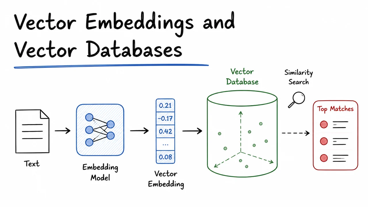
Vector Embeddings and Vector Databases
1. Why Vector Search?
Imagine you type “electric vehicle” into a search box, expecting to find articles about battery technology, charging infrastructure, and the latest EV models. Instead, the results list is filled with documents that contain the exact phrase “electric vehicle” but miss a paper on “Li‑ion breakthroughs for EVs” or a report titled “Charging network expansion.” The problem is not that those documents don’t exist – it’s that your search engine only looks for character‑level matches and does not understand that “EV” means “electric vehicle.” This is the keyword matching trap, and it’s the fundamental limitation that vector search sets out to solve.
Keyword‑based retrieval – the backbone of traditional search engines and databases – relies on inverted indexes that map each term to the documents containing it. When a user submits a query, the system tokenizes the words, finds postings lists, and scores documents by metrics like TF‑IDF or BM25. While fast and interpretable, this approach is brittle: it fails when the vocabulary of the query and the document drift apart, even slightly. Synonyms (“car” vs. “automobile”), paraphrases (“battery advances” vs. “energy storage progress”), or abbreviations (“EV” for “electric vehicle”) all break the exact‑match assumption. Worse, a document can be topically identical but share no terms with the query at all, earning a relevance score of zero. That’s not just a small error – it’s a missing signal that humans handle naturally.
The core insight of modern semantic search is to move beyond sparse, discrete word counts and into a continuous representation space where distance equates to meaning. We learn an embedding function that maps any text – a query, a document title, a paragraph – to a dense vector in . For a query and a corpus of documents , we compute:
Now proximity in this vector space becomes a proxy for semantic similarity. Two sentences that use completely different words can end up as nearby points; irrelevant jargon‑heavy documents land far away. The idea is so powerful that it underlies everything from modern web search to recommendation systems.
How do we measure proximity? The most common choice is cosine similarity, which focuses on the angle between vectors, making it robust to differences in vector magnitude (length). The formula is straightforward:
Values range from (opposite meaning) to (identical direction). In practice, well‑trained embeddings yield cosine similarities above 0.9 for highly relevant pairs and below 0.3 for unrelated content, even when the original texts share no keywords.
Consider our earlier example. A query “electric vehicle” and three candidate documents:
- D1: “EV battery advances” – no words overlap with the query, yet they discuss the same topic.
- D2: “hybrid car” – some conceptual overlap (electrified propulsion) but not a perfect match.
- D3: “petrol engine” – an internal combustion document that happens to contain the word “vehicle” if you squint, but is unrelated in meaning.
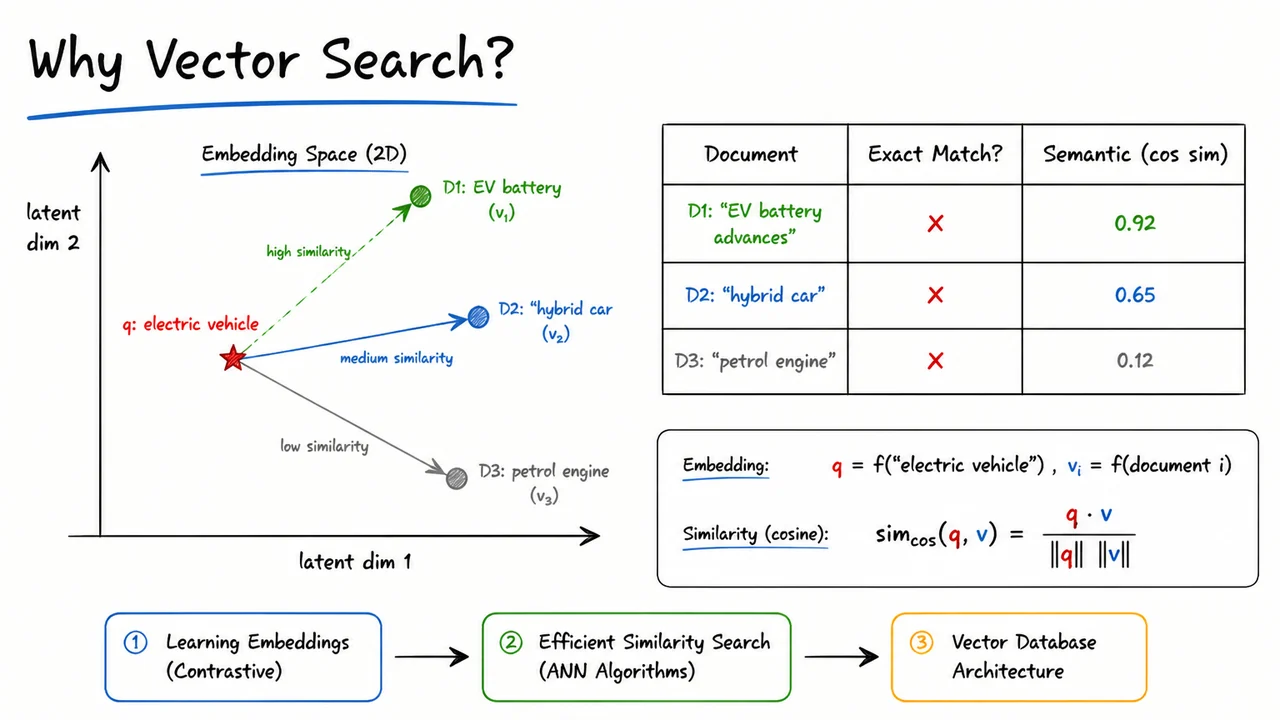
A keyword scorer might rank D3 highest if it contains “vehicle,” while D1 gets ignored entirely. In an embedding space, however, the vector for “electric vehicle” sits close to D1, at a moderate distance from D2, and far from D3. Cosine similarity quantifies this: approximately 0.92, 0.65, and 0.12, respectively. The ranking now reflects actual relevance.
To make this shift from symbolic to continuous representation concrete, the accompanying visual condenses the entire motivation. On the left, a simple 2‑D embedding space (axes labeled “latent dim 1” and “latent dim 2”) acts as a sketch of the true high‑dimensional manifold. A red star marks the query vector for “electric vehicle.” Three document vectors appear as circles: green for D1 (“EV battery advances”), blue for D2 (“hybrid car”), and grey for D3 (“petrol engine”). Dashed arrows connect the query to each document, their lengths corresponding to semantic distance – shortest to D1, longest to D3. This geometric picture immediately communicates that meaning, not dictionary overlap, structures the space.
On the right, a small table drives the lesson home. It lists each document alongside two columns: “Exact Match?” (all ✗) and “Semantic (cos sim)” with scores 0.92, 0.65, and 0.12. The table makes explicit what the arrows imply: keyword matching fails uniformly, while vector similarity correctly separates the topically relevant from the irrelevant. Together, the plot and the table provide a before‑and‑after story for why we invest in learning embeddings and building vector search systems – a bridge from the brittle past to the semantic future.
With this motivation firmly in place, the rest of the lecture unfolds naturally: first, how to learn an embedding function that produces such semantically organized vectors (contrastive learning), then how to search through millions of them in milliseconds (approximate nearest neighbor algorithms), and finally how a modern vector database stitches these components into a scalable, production‑ready system.
2. Embeddings: Dense, Semantics‑Aware Vectors
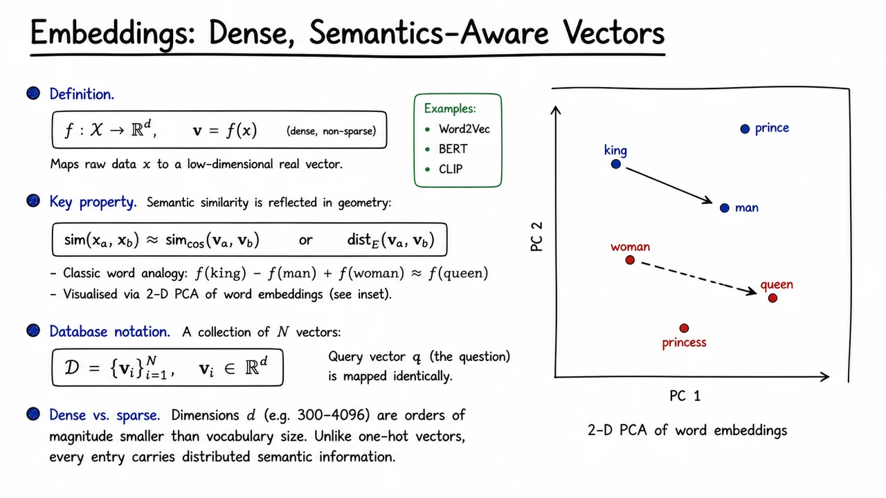
The previous section made it clear that exact‑term matching stumbles when a user’s words differ from the document vocabulary, even if the underlying meaning is identical. The resolution lies in abandoning surface forms entirely and mapping every piece of content—queries, documents, images, products—into a shared vector space where proximity implies relevance. That mapping is an embedding function
which takes a raw item (a word, a sentence, a paragraph, an image) and produces a fixed‑length real vector . The output is dense, meaning every coordinate typically carries a non‑zero value, and the dimensionality (commonly 300–4096) is deliberately much smaller than a naive one‑hot encoding over a large vocabulary. This compactness is not mere compression; it reflects that semantics are distributed across all dimensions in a way that makes vector geometry directly interpretable.
Familiar examples of such embedding functions include Word2Vec for individual words, BERT for sentence‑level context, and CLIP for aligning images with text. Each of these is trained so that semantic similarity is expressed as geometric proximity. In practice we measure proximity with cosine similarity or Euclidean distance:
Because every dimension participates in encoding multiple facets of meaning, small changes in the vector can reflect nuanced differences in connotation, tense, or even analogy. This is fundamentally different from a sparse bag‑of‑words representation, where each dimension is locked to a single vocabulary term and the vector components are counts, not semantic coordinates.
Perhaps the most celebrated demonstration of this property is the word‑analogy arithmetic:
The equation says that the vector offset that separates “man” from “king” (capturing a gendered royal relationship) reappears when we move from “woman” by that same offset, landing near “queen”. More generally, vector differences tend to encode relational concepts: the direction from “Paris” to “France” roughly mirrors that from “Tokyo” to “Japan”. The fact that such algebraic operations in correspond to semantic transformations is the key insight that turns embeddings from a representation into a reasoning tool.
When we scale this to a search system, we store a collection of document vectors
and map every incoming query to a query vector using the same embedding function. Relevance ranking then reduces to finding the vectors in that are closest to under the chosen distance measure. Suddenly, matching “automotive engineer” to “car designer” or “buying a laptop” to “notebook purchase” becomes a nearest‑neighbour problem, not a vocabulary‑alignment puzzle.
The visual here consolidates these ideas by showing a two‑dimensional PCA projection of a small word‑embedding space. While the true embeddings live in hundreds of dimensions, this projection preserves enough structure to make the geometric relationships tangible. Words like “king”, “man”, “woman”, and “queen” appear as labeled points, and directed arrows illustrate the same vector offset reappearing: the arrow from king to man and the arrow from queen to woman are drawn as parallel displacements, giving a concrete picture of how the relational vector is preserved across word pairs. The plot serves as a rapid visual reminder that embeddings learn a space where similarity is distance and analogy is translation—a mental model we will now formalise and exploit when we examine the geometry of embedding spaces in the next section.
3. Geometry of Embedding Space
Having established that dense embeddings map semantics into continuous coordinates, the next natural question is: how do we measure similarity in this latent space? The choice of distance function shapes the geometry of the embedding space and determines what “closeness” actually means. Two metrics dominate modern vector search: Euclidean distance and cosine similarity. Their mathematical relationship — and a crucial equivalence under normalization — directly informs the design of efficient vector databases.
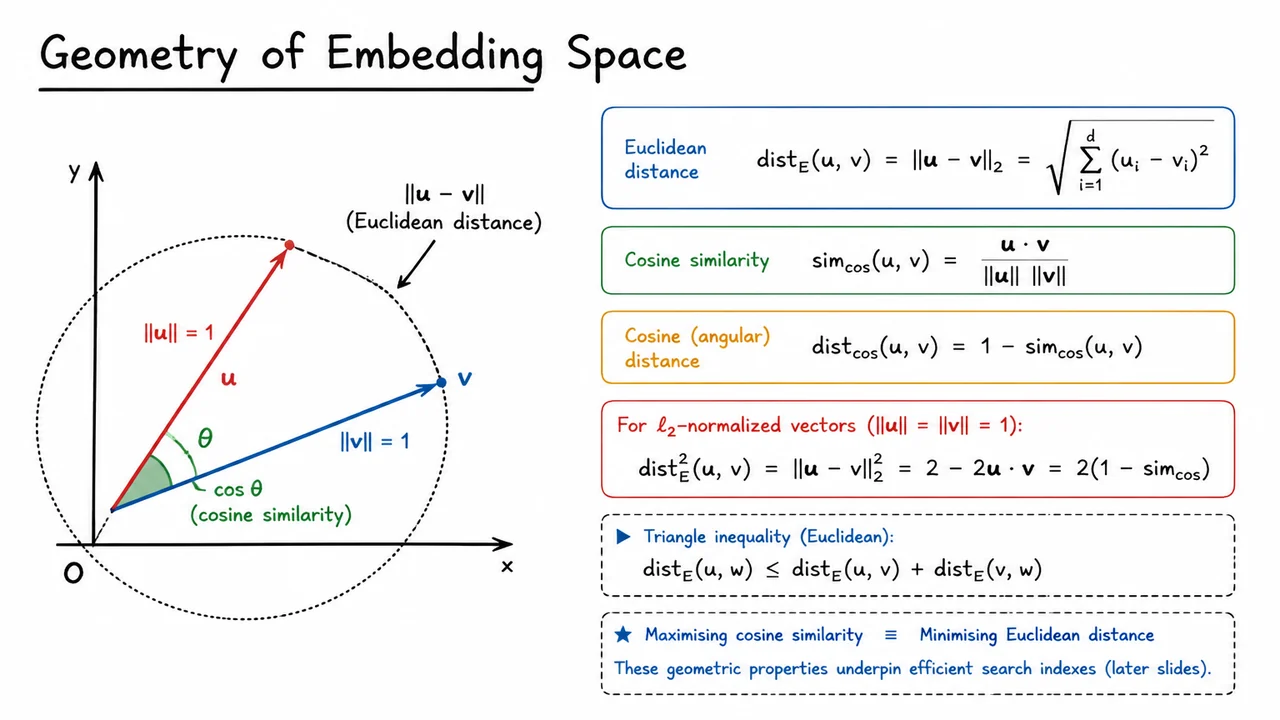
Euclidean distance is the straight‑line (ℓ₂) distance in the embedding space:
It respects both the direction and the magnitude of the vectors: two embeddings can be far apart because they point in different directions, because one has a much larger norm, or both. Cosine similarity, by contrast, focuses purely on orientation, measuring the cosine of the angle between the vectors:
To turn similarity into a distance, one can use the cosine distance:
which ranges from 0 (identical direction) to 2 (opposite). In many embedding pipelines — especially those trained with normalized output heads or followed by explicit ℓ₂‑normalization — the vectors are constrained to lie on the unit hypersphere, i.e. . This normalization has a profound geometric consequence: Euclidean distance and cosine distance become equivalent up to a monotonic transformation.
To see this, expand the squared Euclidean distance for unit‑norm vectors:
Thus, maximising cosine similarity is exactly equivalent to minimising squared Euclidean distance (and therefore Euclidean distance itself, because the square root is order‑preserving). In practice, this means that if you ℓ₂‑normalize all embeddings, a nearest‑neighbor search using inner product, cosine similarity, or Euclidean distance will produce exactly the same ranking. Many vector databases exploit this freedom to store normalized vectors internally and accelerate inner‑product searches.
It is important to keep the magnitude factor in mind when normalization is not guaranteed. For raw embeddings from models that do not enforce unit norm, Euclidean distance can be dominated by differences in vector length rather than semantic orientation, leading to unexpected neighbor results. A standard safeguard is to explicitly normalize before indexing, effectively projecting every point onto the unit sphere and collapsing the two metrics into one. The equivalence, however, is purely a property of the sphere: moving to a sub‑sphere (e.g., by constant‑norm constraints) collapses the distinction between angular and Euclidean proximity.
A second fundamental geometric property is the triangle inequality, which Euclidean distance satisfies:
This inequality is the backbone of many space‑partitioning and pruning strategies that make large‑scale search tractable (think of ball trees or IVF indexes). Cosine distance on arbitrary vectors does not satisfy the triangle inequality, but on the unit sphere it becomes a proper metric — the angular distance (arc length), which is simply . In the normalized regime, therefore, the embedding space is a well‑behaved metric space with a natural spherical geometry, and all the algorithmic machinery built for metrics can be safely applied.
The visual below consolidates these ideas by drawing two normalized vectors on the unit circle. The angle between them is marked, and the chord connecting their tips is explicitly labeled as the Euclidean distance . The law of cosines immediately tells us that the squared chord length equals , which is exactly the identity we derived for . The diagram makes the equivalence tangible: for points on the circle, measuring the straight‑line segment or measuring the angle gives the same information, linked by a monotonic relationship. The triangle formed by the two vectors and the chord also visually enforces the triangle inequality, hinting at the geometric regularity that efficient search indexes will later exploit.
4. Contrastive Loss: Pulling Similar, Pushing Dissimilar
With the geometry of embedding space fresh in mind, we now need a systematic way to impose the desired structure. The intuition is simple: if two items are semantically similar, their vector representations should lie close together; if they are dissimilar, they should be far apart. Translating that intuition into a differentiable training objective is the job of the contrastive loss. Rather than treating each data point in isolation, this loss works on pairs, pulling similar partners together and pushing dissimilar ones apart, but with an important twist: the repulsive force stops once a safe margin of separation is reached. This prevents the model from wasting capacity on items that are already sufficiently distant and avoids the collapse that can occur if all dissimilar pairs are forced infinitely far apart.
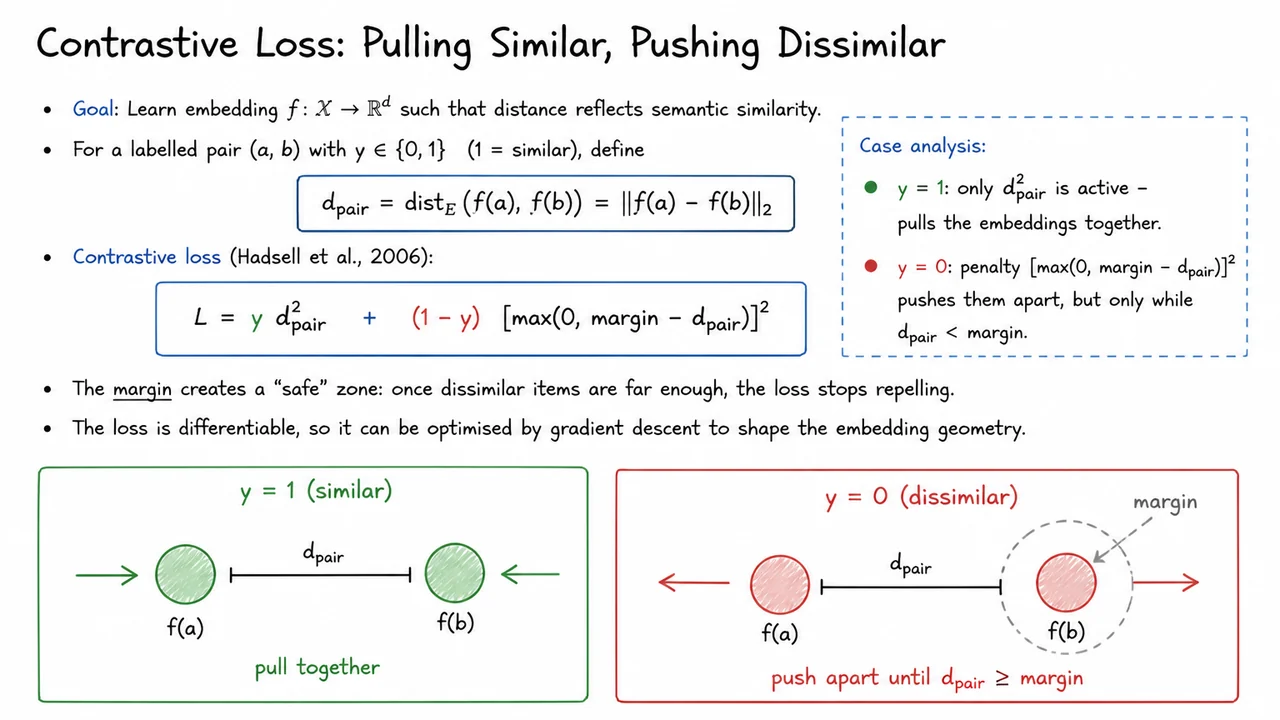
Formally, we aim to learn an embedding function from the input space to a -dimensional Euclidean space such that the L2 distance directly reflects semantic similarity. For a labelled pair with ( for similar, for dissimilar), we define the pair distance as The contrastive loss, introduced by Hadsell et al. (2006), then combines two complementary penalties:
A case analysis reveals the dual nature of this objective. When , only the first term is active, and . This is a convex, quadratic penalty that grows rapidly if the similar pair drifts apart, pulling the embeddings together during gradient descent. When , the similarity flag suppresses the first term, and the second term becomes . This penalty is zero whenever ; in other words, dissimilar items are repelled only while they are inside the margin boundary. Once the distance reaches the chosen margin, the loss cuts off, creating a “safe zone” where the model no longer tries to increase the separation.
Why a margin? Without it, a pure repulsive penalty like or an unbounded hinge would encourage the embeddings of dissimilar items to fly apart without bound, distorting the space and degrading generalization. The margin acts as a computational and geometric guardrail: it says that being “far enough” is sufficient, and any extra distance does not contribute to the semantic objective. The loss is differentiable everywhere (the function has a continuous gradient that goes to zero exactly at the margin), so it can be optimized via standard backpropagation to sculpt the embedding geometry.
This elegant design yields two immediate consequences for training. First, similar pairs experience a continuous attraction that scales quadratically with distance, so the model is especially sensitive to pulling together embeddings that are initially far apart. Second, dissimilar pairs only receive a gradient when their current distance is below the margin; after that, the gradients vanish, and the optimizer focuses its effort on other pairs that still need adjusting. These dynamics make the embedding space naturally cluster semantically coherent items while maintaining well‑defined boundaries between clusters.
The visual below consolidates these ideas into a schematic that captures both the mathematical form and the operational behavior of the contrastive loss. The top two-thirds of the diagram restate the core equations and the two simplified loss expressions for and . The bottom third splits into two panels: the left panel, labelled (similar), shows two filled circles representing embeddings with a distance line annotated ; inward arrows on each circle signal attraction, and a callout reads “pull together”. The right panel, (dissimilar), depicts two embeddings that are initially too close; a dashed circle around one embedding marks the margin boundary, and outward arrows indicate repulsion until the distance meets or exceeds the margin. The colour scheme—green for attraction, red for repulsion, light grey for the margin—provides an at‑a‑glance reminder of the two opposing forces. This way, the diagram does not merely repeat the equations but shows how the loss function orchestrates a mutual attraction–repulsion dance that carves out a semantically organized embedding space, with a safe zone that keeps dissimilar forces in check.
5. Negative Sampling for Scalable Training
After we commit to a contrastive objective that pulls similar points together and pushes dissimilar ones apart, one uncomfortable fact quickly surfaces: the universe of dissimilar items is enormous, often practically infinite. In a million‑item dataset, for every positive pair we would need to push against not one or a handful of negatives, but against all other items to compute the partition function or the full softmax denominator. This is clearly intractable, both in memory and compute, for modern‑scale training runs. The problem was well‑known in the earlier noise‑contrastive estimation (NCE) literature, and it led to a beautiful insight: we can replace the impossible summation over all negatives with a tractable binary classification task that uses only a small number of sampled noise examples.
The core idea of negative sampling is to approximate the contrastive objective by sampling, for each anchor and its positive partner , a set of noise vectors drawn from some noise distribution (often uniform over the dataset). Instead of modeling the full conditional probability of a match, we train a binary discriminator that tells the true pair apart from the noise pairs . The resulting NCE loss is a binary cross‑entropy:
Here is the sigmoid function and measures similarity, which for -normalised embeddings reduces to a simple dot product: . The first term encourages the similarity of the true positive to be high (so that is close to 1, giving a small ), while the second term pushes the similarities of all noise samples low (so that is close to 0, again minimizing the contributions). In effect, we have turned the original softmax‑style contrastive learning into a decoupled binary problem: one genuine observation vs. synthetic negative observations per positive pair.
A crucial theoretical subtlety is that the sampled noise distribution must not be too different from the true distribution of all negatives – otherwise the discriminator could exploit distributional artefacts rather than learning meaningful embeddings. In practice, even a simple uniform noise over the training set works surprisingly well, especially when the number of true negatives is huge and the discriminator’s capacity is limited. The hyperparameter controls the trade‑off: larger provides more accurate estimate of the partition function but increases per‑example training cost. Empirically, modest values of (often between 5 and 20) already produce high‑quality embeddings.
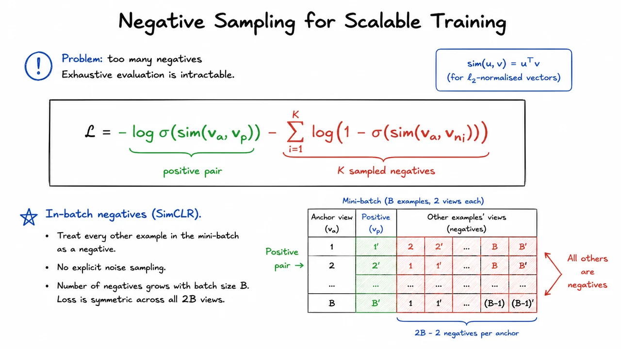
A particularly elegant realisation of this sampling strategy appears in in‑batch negatives, made popular by the SimCLR framework. The observation is disarmingly simple: when training with mini‑batch gradient descent, we already have a batch of size containing many data points. For each example in the batch, the remaining examples (after data augmentation produces two views per original sample) serve as free negatives – no extra noise sampling is needed. The negative sampling is implicit, scaling naturally with the batch size. The loss becomes symmetric across all augmented views, and the effective number of negatives is for each positive pair, which can be substantial when using large batches (e.g., 4096 or 8192). This design turns a computational liability – a large batch is needed for stable training anyway – into a virtue that supplies many informative negatives without an auxiliary sampling mechanism.
However, in‑batch negatives introduce a subtle bias: the negative distribution is now the empirical distribution of the mini‑batch, which may drift over training and is not identically the dataset distribution. This works in our favour because hard negatives (semantically similar but not identical items) that end up in the same batch are especially valuable for learning fine‑grained distinctions. On the flip side, it can cause false negatives when two genuinely similar points are placed in the same batch and one is treated as a negative, slightly violating the contrastive assumption. Many follow‑up works address this with careful label cleaning or by using a momentum encoder to identify and exclude potential false negatives.
The visual below consolidates these two scalable training strategies. A large equation box makes the NCE loss prominent, with its two terms colour‑coded: the positive log‑probability in a reassuring green and the sum of negative log‑complements in a warning red, reinforcing the discrimination task visually. Beneath the equation, a mini‑batch grid depicts the in‑batch negatives: rows represent original data points, each with two augmented views (anchor and positive), and arrows indicate that for a chosen row, every other view from the batch acts as a negative. This sketch makes the gradient flow intuitive – the model must separate the single positive pair from all other points in the batch, which is exactly the binary per‑example optimisation captured by the NCE equation above.
The duality between explicit noise sampling (the NCE loss with draws) and implicit in‑batch negatives (where ) reveals that the two ideas are mathematically unified. Both define a binary cross‑entropy over a positive and a set of negatives. The difference is whether those negatives come from a separate noise generator or from the batch’s own embeddings. Understanding this unification helps us later when we compare training strategies for dense retrievers or when we discuss how vector databases exploit the same embeddings to perform similarity search at scale. For now, the key takeaway is that negative sampling transforms an otherwise hopelessly expensive contrastive objective into a practical, scalable training procedure that fits comfortably within standard mini‑batch deep learning loops.
6. The Exact $k$-NN Search Problem
With a trained embedding model and an arsenal of negative sampling strategies, we can produce vector representations that capture semantic similarity. But the value of these embeddings hinges on an apparently simple retrieval task: given a query vector, how do we efficiently find the most similar items in a database that may hold billions of vectors? The immediate instinct is to define the exact -nearest neighbour (-NN) search problem and solve it directly. That instinct quickly collides with computational reality, and understanding why is the first step toward appreciating the approximate search techniques that underpin modern vector databases.
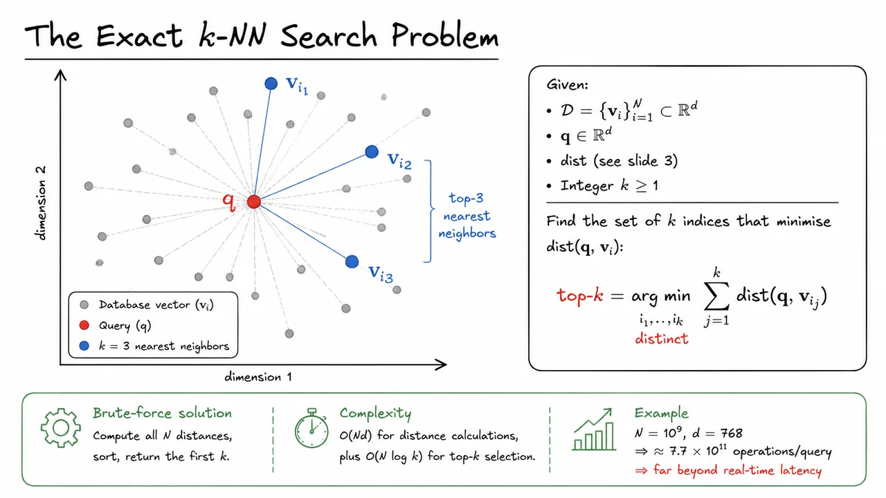
Formally, we are given a database , a query vector , a distance function (such as Euclidean distance, cosine distance, or negative inner product), and an integer . The objective is to retrieve the distinct indices that minimize the aggregate distance from the query:
This formulation cleanly separates the definition of the top- set from any particular algorithm. In principle, the problem can be solved exhaustively by computing for every , sorting the results, and returning the first indices. This brute-force approach is guaranteed to return the exact answer, and for small databases it works perfectly well.
Unfortunately, the brute-force cost scales poorly with both the database size and the embedding dimension . Computing all distances costs floating-point operations. Even with modern hardware, a single query over a billion-scale collection with typical embedding dimensions (say ) demands on the order of arithmetic operations. The subsequent top- selection adds another comparisons, which is negligible by comparison, but the initial distance sweep by itself makes real-time response impossible. Sub-millisecond latency targets are utterly out of reach.
This bottleneck is not a peculiarity of a specific distance measure or a poorly optimized implementation; it is an inherent curse of dimensionality amplified by massive scale. The linear scan inspects every vector, ignoring any structure that the data might possess. In later lectures we will see how the Johnson–Lindenstrauss lemma guarantees that random projections can preserve pairwise distances with high probability, which enables us to work in much lower dimensions. But even with dimensionality reduction, the brute-force scan remains a operation, which is unacceptable when reaches the billions.
A visual consolidation of the exhaustive approach drives the point home. Consider a 2D abstraction of a vector database: a scatter plot with grey dots representing database vectors . A query vector is shown as a distinct red dot. Dashed semi-transparent lines radiate from the query to every grey dot, symbolizing the full distance computation. Among these, the nearest points are enlarged and colored blue, with solid lines connecting them to the query—the desired output. The axes are labeled “dimension 1” and “dimension 2” only to remind us that we are using a low-dimensional projection for intuition; the real database lives in or more.
This picture, while simplified, captures why the exact problem is computationally prohibitive. It makes visible the combinatorial explosion: even a modest-looking point cloud implies a query must consult every database entry. The dashed connections form a dense web that no index can avoid if it insists on exactness. The solid lines to the top- points are the proverbial needle in a haystack; the brute-force method must sift through the entire haystack to find them. That is precisely why the literature shifts its focus to approximate nearest neighbour (ANN) search, where we trade a controlled amount of accuracy for an exponential reduction in query time. Understanding the exact formulation and its limits is the foundation on which those approximate methods are built.
7. The Curse of Dimensionality Strikes Back
Having established that an exact -NN search over vectors in costs —an overhead that already feels heavy—we now turn to a more subtle and devastating obstacle. Even if we could afford that linear scan, the very notion of a “nearest” neighbour begins to erode as the dimensionality grows. This is the curse of dimensionality reasserting itself not through computational cost, but through distance concentration, a geometric phenomenon that corrupts the meaning of proximity.
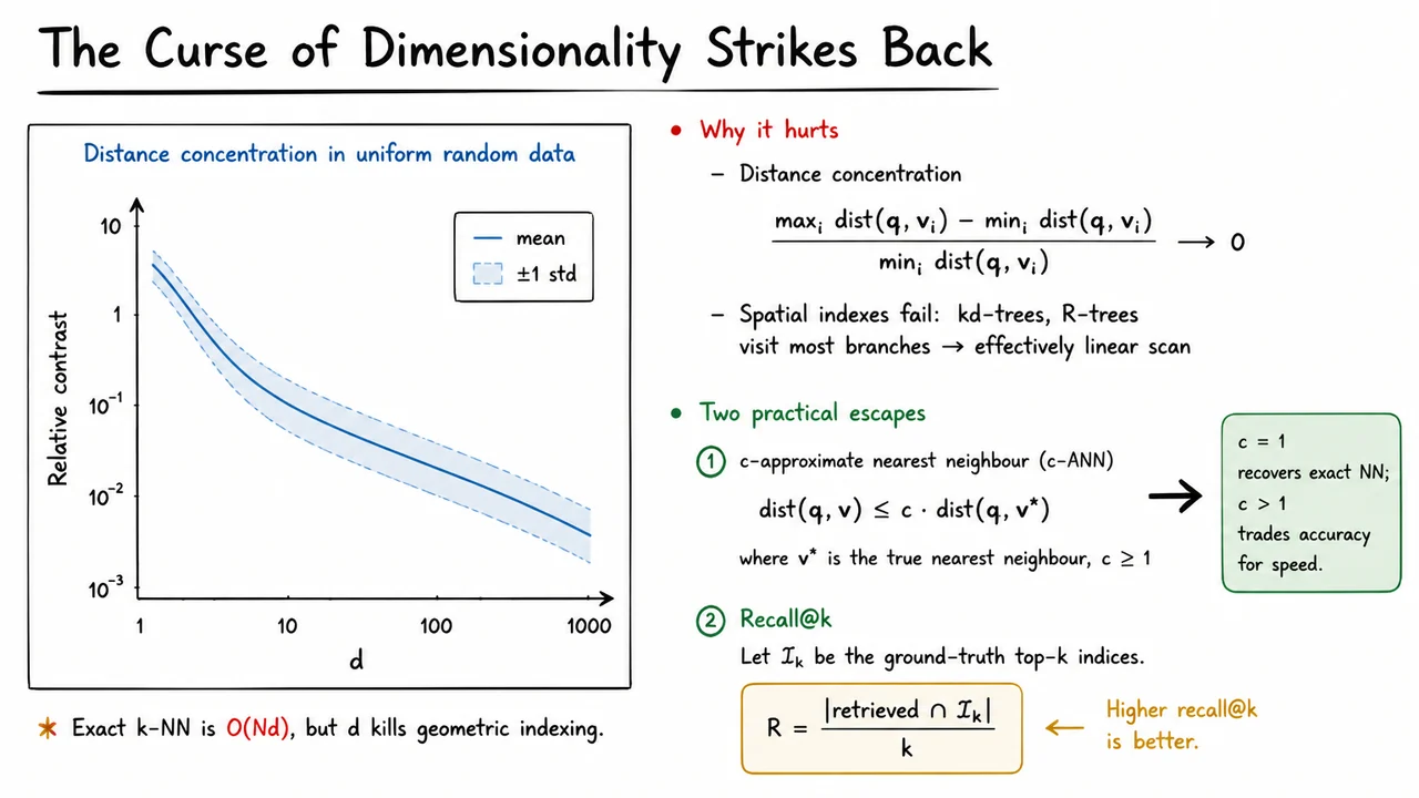
Consider a set of vectors uniformly and independently scattered in the unit cube —or, more generally, any high-dimensional isotropic distribution. For a random query point , we look at the distances to all database vectors . The contrast between the farthest and the closest point can be captured by the relative contrast
When is small—say, 2 or 3—this ratio is comfortably large. The nearest neighbour stands out clearly; its distance might be while the farthest is , giving a ratio of . But as , the ratio shrinks relentlessly toward zero. Why? In high dimensions, almost all pairs of points lie at roughly the same distance from one another; the volume of the space expands so rapidly that most of it is in a thin shell far from any query point. The minimum and maximum distances converge, and the relative difference vanishes. To a search algorithm, every vector looks equally “far”—or equally “close”—and the ranking loses its signal.
This distortion is fatal for the classic spatial indexing structures we might hope to deploy. KD‑trees, R‑trees, and their variants rely on partitioning the space into disjoint regions so that a query can ignore whole branches. In low dimensions, a few well‑chosen splits prune the search dramatically. In high dimensions, however, the query’s hyper‑spherical range overlaps almost all partitions, no matter how clever the splitting strategy. The result is that the index visits a large fraction of the leaves, degenerating into something much closer to a linear scan. Excellent in two dimensions, these structures become useless when vectors are 300‑ or 768‑dimensional embeddings from modern neural models. The curse of dimensionality strikes back, and exact nearest‑neighbour search slips out of reach not because we lack clever algorithms, but because the geometry itself turns hostile.
Practitioners sidestep this collapse by accepting that we do not need the exact nearest neighbour. Two rigorous formulations give us a controlled way to sacrifice perfection for speed. The first is the -approximate nearest neighbour (-ANN). It relaxes the output condition: for a query and some approximation factor , we are allowed to return any database vector that satisfies
where is the true nearest neighbour. When we recover the exact NN; when we permit the answer to be at most times farther away than the optimal one. This single scalar is a powerful knob: a modest (e.g., 1.2) often unlocks enormous speed gains while keeping the geometric error small.
A closely related, and in practice equally important, viewpoint is recall@. Instead of bounding a distance ratio, we measure how many of the true top‑ neighbours our approximate method manages to retrieve. Let be the index set of the ground‑truth nearest neighbours, and let the algorithm return a set of candidates. Then
A recall of means we captured all the true top‑; a lower recall indicates some misses. In vector‑database benchmarks, recall@ is the dominant metric because downstream tasks (semantic search, recommendation) rarely depend on the exact ordering of all items—they just need enough of the relevant ones to appear in the final list. By adjusting the index parameters we can trade recall against query latency, and this trade‑off is what makes modern vector databases practical.
The visual below captures this narrative in one glance. On the left, a line plot charts how the relative contrast decays with dimensionality for uniformly random data. Starting near 3 at , the curve plummets to barely above 0.05 by ; the shaded band of one standard deviation shows just how reliable this concentration is. That plot is the forensic evidence for the curse: the very idea of a “nearest” neighbour loses its separability, explaining why spatial indexes fail and why exact search is folly. On the right, the definitions of -ANN and recall@ are laid out alongside a bold annotation: recovers exact NN, and any trades accuracy for speed. Together, the diagram encapsulates the dual escape from the high‑dimensional trap—mathematical relaxation paired with a measurable, tunable quality criterion—that the rest of the lecture builds upon.
8. Johnson–Lindenstrauss Lemma (JL)
We spent the last section staring into the abyss of high-dimensional spaces, where our geometric intuition evaporates and exact nearest-neighbor search degrades into brute-force scans that are far too slow for real-time retrieval. It’s tempting at that point to believe that high-dimensional embeddings are fundamentally impractical—that the price of expressiveness is an unpayable computational toll. But what if the effective information in those embeddings is far lower-dimensional than the raw embedding space suggests? The Johnson–Lindenstrauss lemma is the theoretical lifeline that tells us exactly that: we can aggressively shrink the dimension while preserving every pairwise distance to within a tiny error, with a target dimension that depends only on the number of points and the desired precision—and, crucially, not on the original dimension.
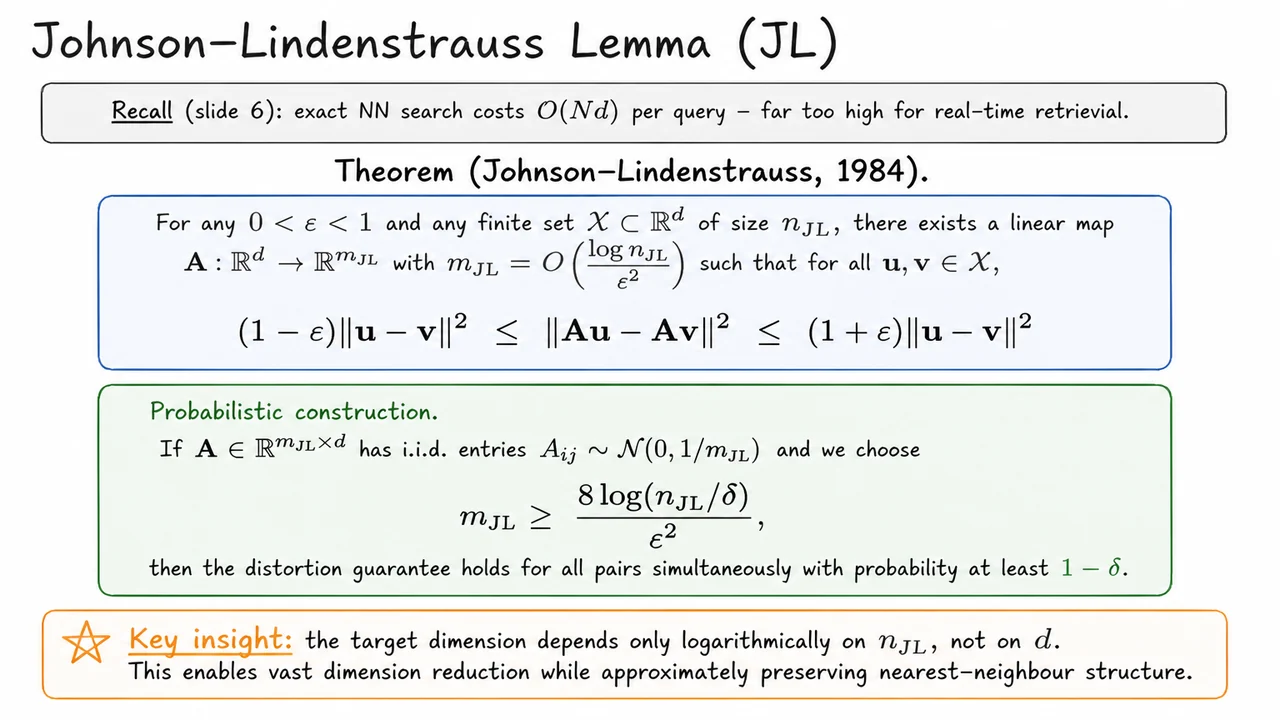
The formal statement (Johnson–Lindenstrauss, 1984) is elegantly simple, yet its consequences are profound. Let be any finite set of points of size , and let . The lemma asserts that there exists a linear map with
such that for every pair ,
In plain words: no pair’s squared Euclidean distance changes by more than a multiplicative factor of . If we set , distances after projection stay within 10 % of their original values. The linear map is the same for all points, so it’s a simple projection onto a lower-dimensional subspace—but with an important twist: the subspace is chosen randomly, not learned from the data. The existence proof is constructive, and the most canonical construction uses a matrix with independent Gaussian entries.
The probabilistic construction is what makes the JL lemma not just a comforting existence result but a practical tool. Take whose entries are i.i.d. samples from . Then for any desired failure probability , if we pick
the distortion guarantee holds simultaneously for all pairs with probability at least . The constant 8 can be tightened in modern variants, but the structural dependence is the same: logarithmic in the number of points, polynomial in , and completely independent of the original dimension . That independence is the lemma’s headline. A billion points in a million dimensions? We still only need dimensions to maintain -distortion with high confidence.
This has immediate, electrifying implications for vector search. If all pairwise distances are preserved within a narrow band, then the nearest-neighbor graph, cluster assignments, radius queries—essentially all proximity-based structures—are approximately preserved as well. The JL lemma provides the theoretical justification for projecting high-dimensional embeddings down to a fraction of their original size before indexing, drastically reducing memory footprint and query-time computation without losing the semantic similarity information we encoded so carefully in the dense vectors. It’s the reason why, in practice, we can store and search billion-scale embedding datasets using only a few hundred dimensions, even when the original embeddings have thousands of dimensions. The lemma doesn’t itself give a search algorithm, but it forms the bedrock on which approximate nearest-neighbor methods are built.
Most treatments of the theorem skip the construction’s intuition. The Gaussian matrix works because each row of performs a random projection onto a one-dimensional subspace whose squared projection magnitude is, in expectation, equal to the original squared norm scaled by . The sum of such independent projections yields an average that concentrates sharply around the true squared distance, and because the matrix acts linearly on the difference vector , the squared norm of the projected difference is precisely . Concentration inequalities for Gaussian random vectors guarantee that the probability of a large deviation from the mean decays exponentially, and a union bound over all pairs yields the desired simultaneous guarantee.
So when the lecturer puts up the slide entitled “Johnson–Lindenstrauss Lemma (JL)”, it’s not just a slab of equations. The visual below is structured as a compressed reference card for the theorem’s three essential layers. The top zone reminds us of the problem from the previous slide: exact NN costs , too expensive. Then it boldly states the theorem. The distortion inequality sits in a soft-blue box, large and centred, making the envelope unmistakable. Directly beneath, a soft-green box walks through the probabilistic construction: the entry distribution and the precise dimension lower bound . Finally, the bottom zone distills the key insight into a single italicised line: the target dimension depends only on , not on the original . That sentence is the entire reason the lemma powers modern vector databases, and the image ensures it lands with the weight it deserves.
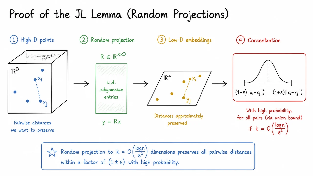
9. Proof of the JL Lemma (Random Projections)
We have just encountered the Johnson–Lindenstrauss lemma in its full statement: any set of points in a high‑dimensional Euclidean space can be mapped into a space of dimension only while preserving all pairwise Euclidean distances within a factor of . The promise is remarkably strong—distortion arbitrarily close to zero, with a target dimension that grows only logarithmically with the number of points—but it begs the question: why does such an embedding even exist? The most elegant justification comes from random linear projections, and proving the JL lemma via random projections reveals why something as simple as multiplying a data matrix by a random matrix is enough to smash the curse of dimensionality.
We begin by fixing the notation. Suppose we have a set of points with potentially enormous. We wish to construct a map such that for every pair ,
with as small as possible. A natural candidate for is a scaled random projection. That is, we draw a matrix whose entries are independent standard Gaussian random variables and define
The scaling by is critical; without it the expected squared norm of the projected vector would grow with . Indeed, for any fixed unit vector , each coordinate of is distributed as , so . Dividing by guarantees that . This unbiasedness suggests that, in expectation, the random projection preserves lengths exactly; the challenge is to show that the actual squared length concentrates sharply around its expectation, uniformly over all pairwise differences.
The concentration argument rests on the tail behaviour of a chi‑squared random variable. For a fixed non‑zero vector , write . Then where i.i.d. The sum follows a chi‑squared distribution with degrees of freedom, and standard sub‑Gaussian or Chernoff‑type bounds give, for any ,
where is a small absolute constant (e.g., from an elementary Markov argument). In words, the probability that the projected squared norm deviates by a factor larger than decays exponentially in the embedding dimension and the square of . This is the probabilistic engine of the JL lemma.
To extend the guarantee from a single vector to all pairwise distances among points, we apply a union bound. There are at most pairs of distinct points. For each difference vector , the probability that its projection distorts by more than a factor is at most . Hence
Choose large enough so that this probability is strictly less than 1. Solving
yields
Thus there exists some realisation of the random matrix for which all pairwise distances are preserved within the desired bounds. The result is non‑constructive in the sense that we do not exhibit a specific matrix, but it guarantees that a random matrix works with high probability—and therefore that such an embedding exists. In practice, we simply sample once and almost surely obtain a valid JL embedding as long as satisfies the above inequality.
Several subtleties are worth highlighting. First, the constant depends on the distribution of the random entries, but the asymptotic form remains unchanged for a wide class of subgaussian distributions, including Rademacher () entries and very sparse random matrices that accelerate computation. Second, the proof summarised here bounds the squared Euclidean norm; using the polarisation identity, the same concentration extends to inner products, which implies that the embedding roughly preserves not only distances but also angles and other similarity measures when appropriate. Third, the union bound that sweeps over all pairs is quite crude—it does not exploit the fact that many difference vectors are correlated—but it is sufficient to obtain the optimal dimension dependence on (there exist matching lower bounds). This union‑bound step is exactly why must grow with : the more pairs we have, the more simultaneous concentration we demand, and the higher the dimension must be to suppress the failure probability for each pair.
The visual that follows crystallises the proof structure. It sketches a cloud of high‑dimensional data points and a random matrix with independent Gaussian entries. Arrows indicate the linear projection , producing a compact set of vectors in . A callout emphasises that pairwise distances are preserved within a factor of with high probability, and a separate badge holds the logarithmic dimension bound that emerges from the union bound over pairs. This diagrammatic summary makes tangible what the probabilistic algebra expresses: a single random projection squeezes a large point set into a surprisingly skinny space while almost perfectly retaining its metric structure. The hand‑drawn aesthetic reinforces the idea that the construction is simple yet powerful—a single multiplication by a random sketch that we can afford to trust in practice.
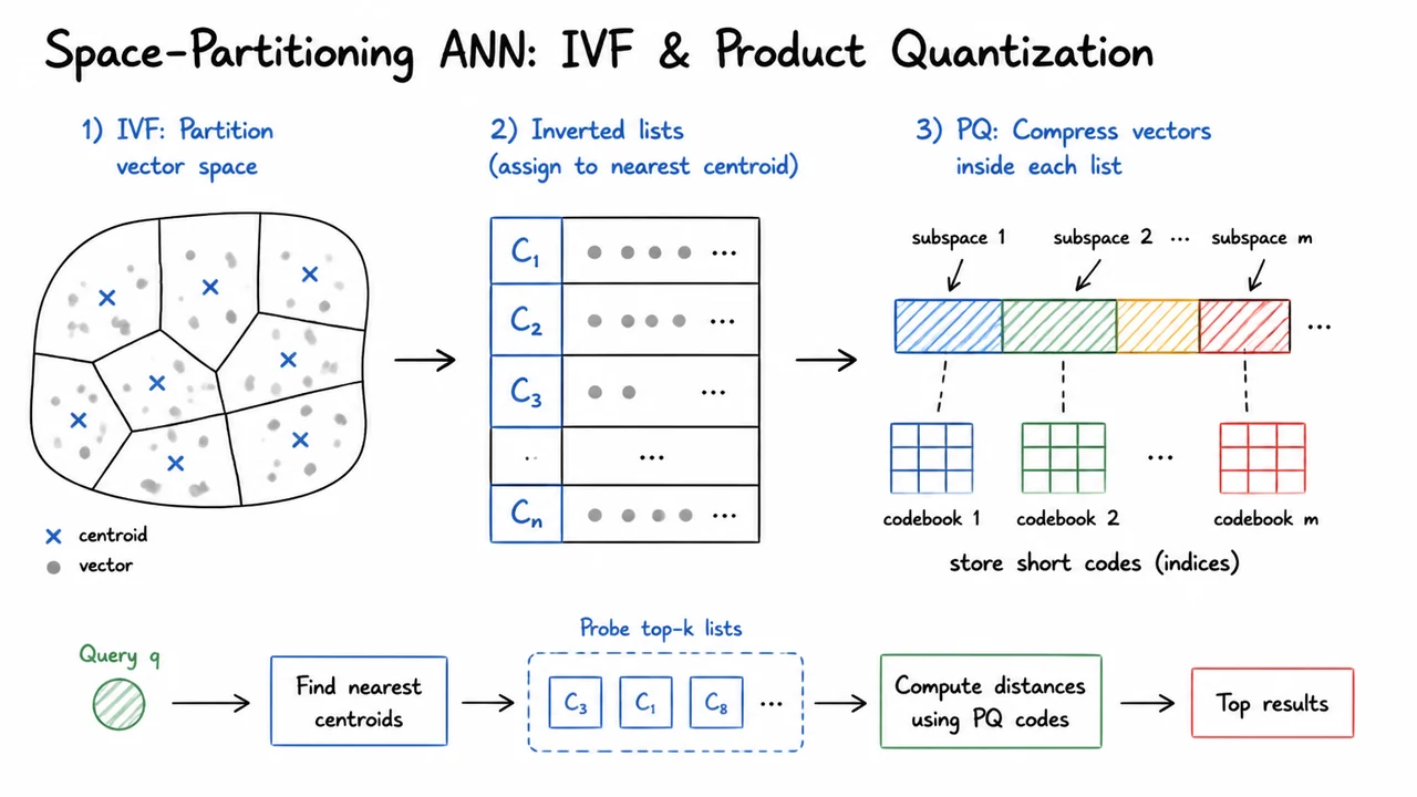
10. Space‑Partitioning ANN: IVF & Product Quantization
The Johnson–Lindenstrauss lemma gives us a powerful guarantee: random projections can crush a high‑dimensional embedding down to dozens of logarithmic dimensions while approximately preserving pairwise Euclidean distances. But knowing distances are preserved does not yet give us a retrieval system that can scan billions of vectors in real time; brute‑force search still scales as , where is the number of stored embeddings. The core of large‑scale vector search is thus approximate nearest neighbor (ANN) algorithms that trade a small, controllable amount of recall for orders‑of‑magnitude speedups. Among the most widely used families of techniques, space‑partitioning methods pre‑process the dataset into discrete regions so that only a fraction of the vectors are examined during a query. Two canonical building blocks are the inverted file index (IVF) and product quantization (PQ); when layered together they form the backbone of industrial engines like Faiss.
The idea behind IVF is deceptively simple. First, the vector space is partitioned into clusters, usually via k‑means on the database vectors, producing a set of coarse centroids . Every database vector is assigned to its nearest centroid, and we build an inverted list for each centroid containing the vector IDs (and optionally the vectors themselves) that belong to that cluster. At query time, the search engine computes the distance from the query to each coarse centroid, selects the closest centroids (the probe parameter), and then exhaustively scans only the vectors in those lists. The speedup factor is roughly ; probe is blazingly fast but risks missing the true nearest neighbor if it lies in a different cluster – a failure mode known as the “edge problem.” In practice, modest (e.g., 8–128) combined with a large (tens of thousands) yields high recall while still being orders of magnitude faster than a full scan. But IVF alone stores every vector in its original full‑dimensional form, which consumes immense memory for billion‑scale collections.
This is where product quantization enters as a compression scheme that can shrink vectors by an order of magnitude while still supporting fast approximate distance calculations. The key insight is to split each -dimensional vector into disjoint sub‑vectors of dimension . For each subspace, a separate codebook of centroids is learned (again via k‑means) using only that subspace of the training vectors. Each full vector is then encoded by the indices of the nearest subspace centroids – an -tuple of -bit integers. The memory per vector drops from bits to bits, achieving a compression ratio around 10–30× for typical settings. To compute the distance between a query and a PQ‑encoded database vector, we exploit asymmetric distance computation: pre‑compute a table of distances between each query sub‑vector and all centroids of the -th subspace, then approximate the Euclidean distance as the sum of the appropriate table entries. The approximation error – the quantization distortion – is bounded and can be controlled by the codebook size.
Individually, IVF reduces the number of candidates, and PQ reduces the storage and distance computation cost per candidate. The real magic happens when they are combined, as in the classic IVFADC index. After the coarse partitioning, instead of storing the raw vectors in each inverted list, we store their residuals relative to the centroid of the cluster. These residuals are much more concentrated around zero, making product quantization far more accurate than quantizing the original vectors directly. The query is also transformed into a residual relative to each probed centroid, and the approximate distance becomes , where is the PQ reconstruction of the residual. This two‑level structure – coarse partitioning followed by compressed residual encoding – yields a system that can search a billion vectors in memory on a single machine with sub‑millisecond latency and >95% recall.
The diagram below distills this layered architecture into a single glance. It will show a 2D space partitioned into Voronoi cells around coarse centroids (the IVF stage) with a magnified view inside one cell, where the residual vectors are split into sub‑vectors and each sub‑space is encoded by its own PQ codebook. A query point is plotted, and arrows illustrate how the search first identifies the closest centroid, then computes the approximate distance to the encoded vectors using the precomputed sub‑distance tables. This compact visual summary reminds us that space‑partitioning ANN is not a single monolithic trick but a careful fusion of vector compression and spatial pruning – a design that directly addresses the twin bottlenecks of memory bandwidth and compute that dominate large‑scale retrieval.
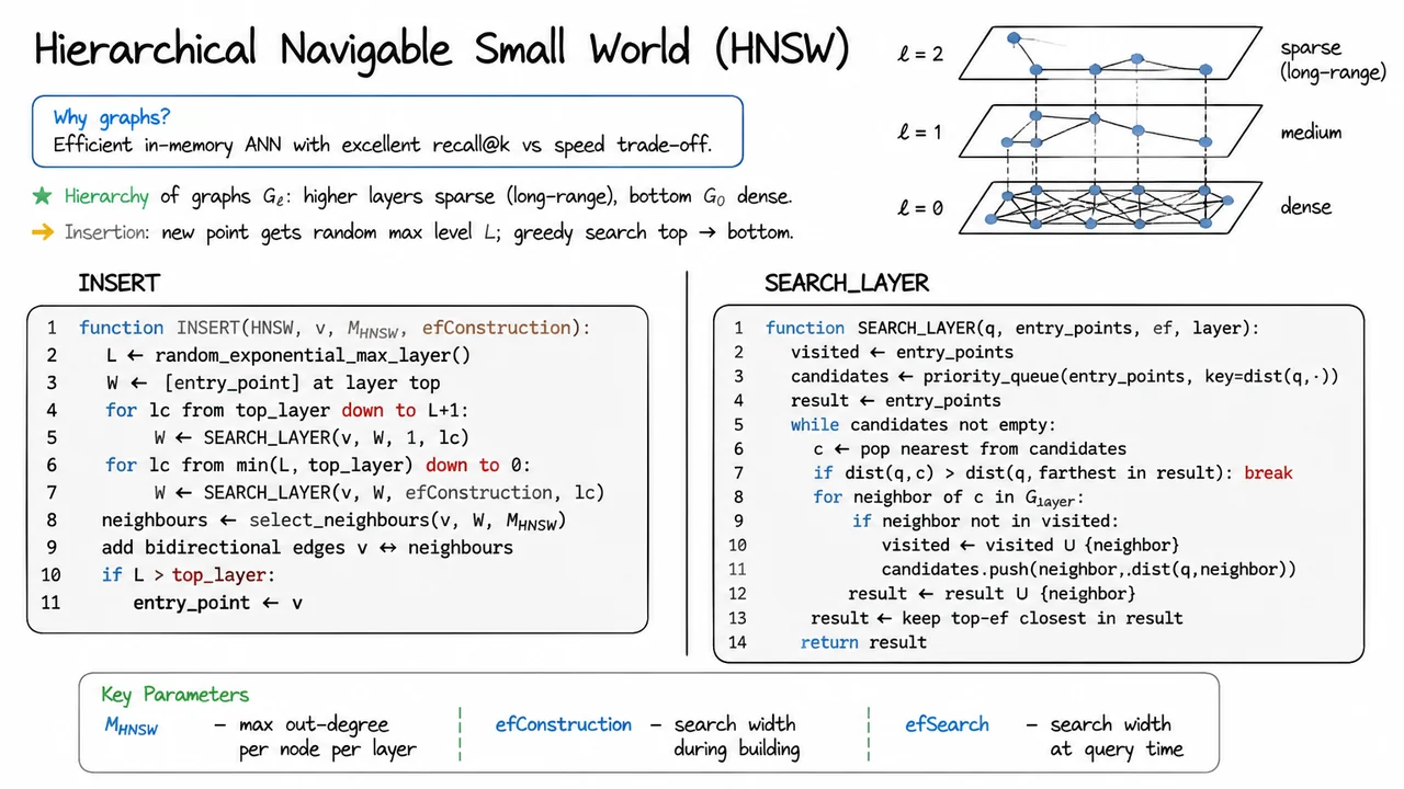
11. Hierarchical Navigable Small World (HNSW)
While space‑partitioning methods such as IVF and product quantization pack vectors into clusters or compressed codes to tame exact search, they impose rigid boundaries that can cause a sharp drop in recall when a query lands near a partition edge. Graph‑based approximate nearest‑neighbor (ANN) algorithms take a fundamentally different approach: they model the dataset as a navigable small‑world network where each vector is a node and edges encode proximity, so a greedy walk can hop from one node to another, progressively refining the estimate of the nearest neighbors. In theory, a small‑world graph with the right degree distribution lets a search skip across large regions of the space in only a few steps. The challenge is building such a graph efficiently and preventing the greedy walk from getting trapped in a local minimum far from the true nearest neighbors.
The Hierarchical Navigable Small World (HNSW) algorithm solves both problems by constructing a multi‑layer graph, inspired by the skip‑list data structure. Instead of a single flat graph, HNSW maintains a hierarchy for . The bottom layer contains every node and is dense, with edges connecting each point to its nearest neighbors; it captures the fine‑grained local structure. Higher layers contain a sparser subset of nodes—each node appears up to its randomly assigned maximum layer —and edges tend to be longer, forming expressways that jump across the space. The random assignment uses an exponential distribution so that the probability of a node reaching layer decays rapidly with . This yields a pyramid: a few high‑degree “hub” nodes in the upper layers and many low‑degree nodes confined to the bottom.
The core insertion routine, often called INSERT, places a new vector into the hierarchy in a top‑down fashion. First, draws a maximum layer from the exponential distribution. Starting from the global entry point at the topmost layer, the algorithm performs a greedy search downward: at each layer above , it uses a simple 1‑greedy step (ef = 1) to update the nearest candidate, and from layer down to 0, it runs a wider SEARCH_LAYER with a parameter . The result is a set of candidate neighbors for at each layer. The algorithm then selects up to of them—typically using a heuristic that avoids connecting to nodes that are too close to each other, keeping the graph navigable—and adds bidirectional edges. If exceeds the previous top layer, becomes the new entry point. This construction ensures that every node finds its place in the hierarchy while maintaining the small‑world property: the graph is built incrementally, yet the final structure supports fast, logarithmically scaling searches.
Query‑time search mirrors the insertion logic but is read‑only. The search begins at the top‑layer entry point and greedily descends layer by layer, using a beam search with width (the same SEARCH_LAYER subroutine). The beam retains the closest candidates seen so far, expanding from the nearest unexplored node. Once the distance to the current candidate exceeds the distance to the farthest element in the result set, the search at that layer terminates—a standard early‑stopping condition for nearest‑neighbor beam search. This strategy rapidly narrows the search region, and the final beam at layer 0 produces the approximate top‑ results. Because the top layers are sparse and contain long‑range edges, the query can jump to the correct neighborhood with only a handful of distance computations, and the dense bottom layer refines those candidates to high accuracy.
The power of HNSW lies in its explicit, tunable knobs that let practitioners trade off recall, speed, and memory. Three parameters govern behavior: the maximum out‑degree per node per layer (which also sets the effective degree at layer 0 by a doubling rule), the construction search width , and the query‑time search width . Increasing improves recall at the cost of more memory and slower insertion; raising builds a higher‑quality graph but prolongs index construction; and varying is the primary runtime lever—larger beam widths increase recall almost monotonically while latency grows roughly linearly with . This clean separation between index‑building effort and query‑time performance makes HNSW especially attractive for production systems that can afford offline index construction but demand low‑latency online queries.
The visual below consolidates these ideas into a compact reference that mimics a developer’s notebook. The layout splits into two columns: the left column holds the INSERT pseudocode, and the right column the SEARCH_LAYER routine, each in a light, monospace‑styled block. Above them, bold headings label the two functions, and a thin vertical separator guides the eye. Beneath the code, a small parameter key lists , , and with short descriptions, reinforcing the tunable nature of the algorithm. Tucked into the top‑right corner, a schematic of the layered graph itself appears: three horizontal planes marked , , and , with scattered nodes connected by sparse edges on the upper levels and a dense web at the bottom. This inset captures the hierarchical structure at a glance—the same structure that the pseudocode manipulates—and serves as a visual anchor that ties the algorithmic details back to the geometric intuition of expressways and local refinement.
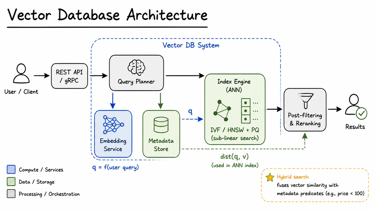
12. Vector Database Architecture
Deep within a production search stack, the HNSW graph or IVF‑PQ index is only one piece of a larger puzzle. An approximate nearest neighbour algorithm can route a query to the top‑ items in milliseconds, but real systems rarely ask questions of the form “give me the 10 most similar vectors” alone. A user might want articles published in the last week, products with a price under $100, or images that belong to a specific category. They might submit raw text, an image, or a hybrid signal, and they expect results that respect both semantic similarity and hard constraints. Bridging the gap between a raw user request and a low‑latency, filtered similarity search over billions of vectors demands a carefully architected pipeline: the vector database.
At the heart of this architecture lies the distinction between search and retrieval. An ANN index answers the narrow question “given a vector , locate vectors that minimise ”, but it knows nothing about the domain semantics of the query, nor about any auxiliary predicates attached to the data. A production vector database therefore wraps the index in a set of services that handle data ingress, embedding transformation, metadata storage, plan optimisation, and result re‑ranking. The goal is to expose a simple query interface—typically REST or gRPC—that feels declarative to an application, while internally orchestrating a carefully choreographed flow across memory‑optimised indices and predicate‑aware stores.
The first component that touches a user query is the Embedding Service. It accepts raw input (text, images, audio) and applies a pre‑trained encoder to produce a dense vector . This step must be both fast and semantically consistent with the vector representations that were used to build the index. In many systems the embedding model is a transformer fine‑tuned via contrastive objectives; any drift between training and inference—due to model updates or normalisation mismatches—will silently degrade recall, so the service is often versioned and cached. The freshly minted is a point in the same high‑dimensional space as the indexed documents, ready to be compared via some distance metric.
Meanwhile, the Metadata Store holds the scalar attributes that make hybrid search possible. It can be a traditional database, a columnar store, or a custom inverted file keyed to document IDs. When a query arrives with a predicate such as price < 100 AND category = "book", the Query Planner must decide whether to apply this filter before vector search (pre‑filtering), after (post‑filtering), or both. Pre‑filtering reduces the candidate set and can prevent the ANN index from returning vectors that will ultimately be discarded, but if the filter is too restrictive it may force an exhaustive scan; post‑filtering is simpler but can waste index lookups on irrelevant items. Modern planners use statistics and dynamic sampling to choose a strategy, then feed the surviving candidates through the ANN engine.
That Index Engine is where the lessons of slides 6–11 become concrete. The engine houses one or more ANN indexes—IVF clusters, HNSW graphs, or product‑quantized codes—and accesses them with memory‑mapped files or in‑process data structures to minimise I/O. When the Query Planner dispatches a search, it passes plus any metadata‑derived ID list. The index engine computes for a subset of vectors, using efficient distance kernels (SIMD, pruned computations) and navigates the graph or inverted files to return a short list of candidates. Thanks to the sub‑linear scaling properties of these indices, query time stays manageable even when billions of vectors are stored, provided the index’s internal structures are kept compact (e.g., via product quantization). Crucially, the engine does not interpret scalar predicates; it merely answers a vector similarity query with an optional exclusion set, returning a candidate list together with precomputed distances.
That candidate list then flows into the Post‑filtering & Reranking stage. Here, any remaining metadata conditions that were not handled by pre‑filtering are applied, and a more refined scoring function can be computed—perhaps a weighted combination of vector similarity and BM25 text score, or a learned rescoring model. The final step is to sort, trim to the requested top‑, and return the results along with their scores and metadata back through the Query Planner to the client. This layered design allows the system to combine the speed of approximate vector search with the precision of exact predicate evaluation, all while maintaining transactional consistency when documents are updated or deleted.
A unifying abstraction emerges: the vector database is not just an index but a query processor that treats vector similarity as a first‑class operator alongside traditional filters, aggregates, and hybrid scores. The REST/gRPC frontend, the embedding service, and the metadata store are all first‑class citizens; together they turn a raw user utterance into a vector and a set of constraints, route that combination through the ANN index, and refine the output before it reaches the user. The sub‑linear theoretical guarantees that Johnson–Lindenstrauss and graph navigability provide are only fully realised when this entire pipeline respects the latency budget—typically a few tens of milliseconds—from end to end.
The architectural diagram below compresses this entire flow into a directed visual narrative. It begins with a user/client icon whose request enters through a REST/gRPC gateway, then immediately reaches the Query Planner—the brain of the operation. Three diverging arrows capture the planner’s key interactions: one thick arrow sends the raw query to the Embedding Service (highlighted in light blue, symbolic of neural computation) where is computed; another arrow communicates with the Metadata Store (a green database cylinder) to retrieve qualifying documents or pre-filter identifiers; the third points to the Index Engine (shaded green, labelled with “IVF / HNSW + PQ (sub‑linear search)”) which is the vector search muscle. A dashed line from the Embedding Service delivers to the Index Engine, while a dashed line from the Metadata Store conveys predicates to the Post‑filtering & Reranking box. The Index Engine’s output also feeds into that processing stage, where distances and metadata are fused. Finally, an arrow leads to the Results, represented by a user icon with a checkmark, completing the pipeline. A surrounding dashed rectangle groups the internal components under the “Vector DB System” banner, underscoring that all these services work as an integrated whole.
Looking at this assembly, you can see why empirical benchmarks of vector databases focus not merely on raw queries‑per‑second of the ANN index, but on end‑to‑end recall and latency under mixed workloads that include filtering, updates, and concurrency. The choice of index algorithm (HNSW vs IVF) and the strategy for pre‑filtering become knobs that trade off memory, recall, and query cost, and the diagram makes explicit where each knob lives. With this architecture in mind, the next section will examine the quantitative trade‑offs that real deployments face, interpreting recall‑versus‑speed curves and the impact of practical constraints like index build time and memory pressure.
13. Benchmarks: Recall vs
The careful engineering of index structures—inverted files, product quantization, navigation graphs—gives vector databases their speed and scalability. But architecture alone does not tell us how a given design behaves under real query loads. We need to measure the trade-off between accuracy, throughput, and memory in a way that generalizes across data types and deployment constraints. The community has converged on a set of standard benchmarks that expose this trade-off, and the resulting curves are among the most useful diagnostics a practitioner can consult before choosing an approximate nearest neighbor (ANN) index.
The three quantities that matter most in production are Recall@k, Queries per Second (QPS), and index memory consumption. Recall@k—usually k = 10—captures the fraction of true top‑k nearest neighbors returned by the approximate index, compared to an exact brute-force scan. It is the primary signal of retrieval quality. QPS measures the system’s throughput under a continuous stream of queries, typically reported on a single machine to factor out distributed scaling effects. Memory footprint accounts for the storage cost of the index itself, expressed either in bytes per vector or relative to the raw uncompressed vectors. A well-chosen index pushes the Pareto frontier: it will not be best at all three simultaneously, but it will offer a sweet spot that matches the application’s requirements.
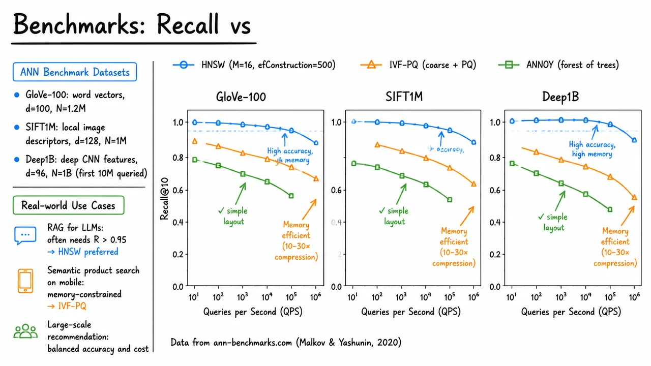
Three canonical approaches stand out in the literature, each embodying a distinct design philosophy. HNSW (Hierarchical Navigable Small World) builds a multi‑layered graph where a greedy search can jump from coarse to fine neighborhoods with logarithmic complexity. It stores the full vectors alongside the graph edges, so its accuracy is exceptional—often Recall@10 > 0.95—but its memory use is essentially 1× the raw vector storage plus edge overhead. IVF‑PQ combines an Inverted File with Product Quantization: a coarse quantizer partitions the space into cells, and the residual vectors within each cell are compressed with compact PQ codes. The index size can be 10–30× smaller than the raw data, enabling high QPS, but the quantization noise caps recall around 0.8–0.9. ANNOY, a forest of random projection trees, trades robustness for simplicity; it achieves moderate recall (~0.8) with very low memory and high QPS, but it struggles to reach the high‑accuracy plateau that modern generative applications demand.
These trade‑offs are revealed on standard datasets that probe different dimensionalities and data distributions. The GloVe‑100 set contains 1.2 million 100‑dimensional word embedding vectors; SIFT1M provides 1 million 128‑dimensional image descriptors; and Deep1B offers the ultimate stress test with 1 billion deep CNN feature vectors (96‑dimensional, though benchmarks often query the first 10 million). All three datasets are publicly used by the ann‑benchmarks framework (Malkov & Yashunin, 2020), ensuring reproducibility.
A typical benchmark sweep tunes each algorithm’s construction and search parameters—for HNSW, the connection degree and the search‑time ef‑factor; for IVF‑PQ, the number of coarse centroids and PQ subvectors—to sample points along the accuracy–speed curve. The result is a family of points per algorithm, plotted as Recall@10 on the vertical axis against QPS on a logarithmic horizontal axis. For HNSW, the curve hugs the top of the plot (>0.95 recall) across a wide range of QPS, but the annotation reminds us that this high quality comes at the cost of index memory comparable to the raw vectors. IVF‑PQ, on the other hand, yields a lower recall ceiling (roughly 0.85–0.9) but pushes the QPS far to the right thanks to the compact codes and inexpensive distance computations. A dashed line or callout often marks the memory‑efficiency gain, e.g., “10–30× compression.” ANNOY typically carpets a middle ground, delivering decent recall at high QPS with a small, simple memory layout, but never crossing the 0.9 barrier that many precision‑critical tasks require.
From these curves, real‑world deployment rules of thumb emerge. Retrieval‑Augmented Generation for large language models, where a single missed document degrades the generated answer, almost mandates recall above 0.95; HNSW is the go‑to choice despite its memory appetite. On‑device semantic search on mobile platforms, where memory and battery are strict limits, naturally favors IVF‑PQ and its compact representations. Large‑scale recommendation systems, serving millions of users with tight latency budgets, often pick a balanced configuration that sits somewhere between HNSW and IVF‑PQ on the Pareto frontier, sometimes blending multiple indices.
The visual that accompanies this discussion distills the entire empirical landscape into a single, scan‑nable figure. Across three side‑by‑side panels—one for each benchmark dataset—the same three curves appear: HNSW in blue with circle markers, IVF‑PQ in orange with triangle markers, ANNOY in green with square markers. The axes are clean: Recall@10 from 0.0 to 1.0 on the y‑axis, and Queries per Second on a log‑scaled x‑axis. The HNSW curve stays high and stable, with a small annotation “High accuracy, high memory” and a blue dashed line indicating 1× raw vector memory. IVF‑PQ runs lower on recall but stretches to the far right; an orange callout “Memory efficient (10–30× compression)” appears near its rightmost points. ANNOY’s green curve sits between them, labelled “simple layout.” A compact legend at the top of the first panel unifies the color coding, and a tiny footnote “Data from ann‑benchmarks.com (Malkov & Yashunin, 2020)” cites the source. This arrangement lets the viewer absorb the trade‑off logic at a glance: no single algorithm dominates, and the right choice depends on whether your priority is near‑perfect recall, memory frugality, or a balanced profile.
14. Challenges and Emerging Directions
While benchmarks such as recall-vs-latency curves expose the practical performance landscape, they also reveal deeper systemic limitations that current vector databases still struggle to overcome. Pushing vector search from demonstration‑scale workloads to truly production‑grade, ever‑changing, multi‑modal, billion‑item deployments requires solving a set of interconnected problems that live squarely at the intersection of information retrieval, systems, and representation learning. In this section we survey the major open challenges and the emerging research directions that aim to close the gap between prototype and platform.
The first challenge is filtered vector search, where an approximate nearest neighbor query must be combined with SQL‑style predicate filters. For example, a product search might ask for “shoes” (a text filter) that are visually similar to a given image. The naïve strategies—pre‑filtering (applying the filter first, then running ANN on the survivors) and post‑filtering (running ANN, then discarding results that do not match the filter)—each have sharp failure modes. Pre‑filtering can shrink the candidate pool so drastically that the ANN step no longer has enough relevant neighbors to return, while post‑filtering wastes compute on high‑similarity items that will be thrown away. The fundamental difficulty is that the vector index and the metadata index are separate data structures with no shared cost model; cardinality estimation becomes brittle, and the optimal order of operations depends on both the selectivity of the predicate and the geometry of the embedding space. Researchers are now developing adaptive placement strategies that use lightweight cost models, learned cardinality estimators, or even join‑style reordering that blends ANN traversal with predicate evaluation on the fly.
A second thorny issue is incremental updates. Modern graph‑based indexes like HNSW are constructed assuming a static dataset; edges are optimised once and then frozen. Under continuous inserts and deletes, the graph’s navigability degrades: newly inserted vectors may form dangling subgraphs, and removal of popular hub nodes can fragment the structure, causing recall to drop over time. Simple workarounds such as periodic full rebuilds become prohibitively expensive for large, continuously written data. Emerging solutions adapt ideas from log‑structured merge trees: maintain a small mutable in‑memory graph layer and a larger immutable on‑disk component, periodically merging them in the background. Others explore incremental repair algorithms that locally re‑wire edges after deletions, or frozen‑layer architectures where only the upper, coarse‑grain levels of a hierarchical graph are updated online. The challenge is to keep query latency stable and recall high without pausing the service for rebuilds.
Billion‑scale, beyond‑memory workloads push the systems dimension even further. HNSW’s traversal pattern is notoriously reliant on random memory access; when the graph no longer fits in RAM, each hop can incur a disk seek, ballooning latency by orders of magnitude. Disk‑resident graph indexes must carefully schedule random reads, often by using NVMe SSDs that offer high IOPS and exploiting spatial locality through graph partitioning. Hierarchical sharding splits the dataset into manageable chunks, keeping the upper navigation layers in fast memory while relegating dense lower layers to disk. An orthogonal line of attack is aggressive quantization (scalar, product, or vector quantization) that compresses the vectors themselves so that more of the graph can reside in memory, but this trades off distance accuracy against footprint. Finding the sweet spot between compression, sharding granularity, and I/O scheduling remains an open systems problem.
On the modelling side, multi‑modal embeddings introduce a representation mismatch. Most embeddings are still trained in isolated per‑modality spaces: a text encoder and an image encoder may each produce 768‑dimensional vectors, but there is no guarantee that a query about a “red sneaker” in text and an image of a red sneaker land close together. Joint embedding spaces like those produced by CLIP align modalities through contrastive training, yet these spaces often sacrifice fine‑grained intra‑modality discriminability. In a vector database, supporting cross‑modal retrieval robustly requires either index‑fusion strategies that merge multiple per‑modality indexes at query time, or a single unified index over a shared embedding space. The research direction here is toward more expressive joint spaces that can preserve modality‑specific detail while enabling seamless cross‑modal similarity, as well as fusion techniques that can dynamically weight modality contributions depending on query type.
Beyond fixed partitioning schemes, the idea of learned indexes questions the entire hand‑crafted design pipeline. Instead of engineering a partitioning algorithm like IVF or a quantizer like PQ, we can train a neural network to directly map a query to a shortlist of candidate vectors (Differentiable Search Index, DSI) or to predict partition boundaries that adapt to the data distribution. Learned distance functions can replace generic cosine or Euclidean metrics with a tiny model that captures domain‑specific similarity. While these methods have shown impressive recall–latency trade‑offs in experimental settings, they introduce new costs: training the index requires a substantial amount of data and compute, adaptation to online data drift is non‑trivial, and the inference overhead of a neural partitioner must be carefully balanced with the latency it saves. Making learned indexes practical for production is a vibrant area of systems–ML co‑design.
Finally, all of these ambitions are gated by cost‑efficiency. High query‑per‑second (QPS) rates under strict latency budgets push the need for hardware acceleration (GPUs, TPUs, FPGA‐driven similarity computation) and extreme quantization. Yet naive GPU‑offloading can saturate the PCIe bus, and aggressive quantization degrades recall unless the distortion is carefully managed. The emerging direction is hardware‑conscious design: kernels that fuse distance computation with graph traversal, mixed‑precision storage that keeps high‑precision vectors only for the top few graph layers, and auto‑tuning frameworks that jointly optimise recall, latency, and dollar cost.
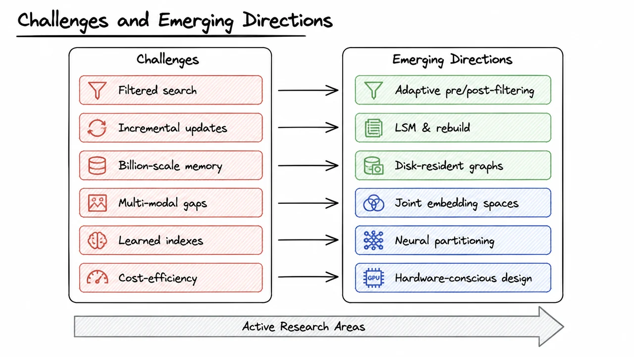
The visual below captures this landscape as a paired mapping between six core challenges and their corresponding research directions. On the left, red‑toned boxes list the obstacles—filtered search, incremental updates, billion‑scale memory limits, multi‑modal gaps, sub‑optimal hand‑crafted indexes, and cost pressure. On the right, green‑ and blue‑toned boxes outline the emerging solution families: adaptive pre‑/post‑filtering, log‑structured merges and background rebuilds, disk‑resident graphs, joint embedding spaces, neural partitioning, and hardware‑conscious design. Curved connectors emphasize that each line of work is a direct response to a specific pain point, while the bottom arrow reminds us that these are active, fast‑moving research areas. The diagram does not list every detail—rather it organises the space so that the reader can see at a glance how each theoretical or systems challenge spawns a coherent thread of engineering and algorithmic innovation, exactly the kind of matrix that a practising vector‑database architect must internalize when choosing what to build and what to borrow.
15. Summary: The Vector Search Landscape
Building a production-grade vector search system is a multi‑layered challenge that touches representation learning, information retrieval theory, and distributed systems engineering. After dissecting each layer in isolation, it is helpful to step back and see how they fit together into a coherent landscape. That landscape is defined by a central tension: we want to search over semantics, not mere tokens, and we want that search to be fast and accurate at the scale of millions or billions of items.
The journey begins with dense vector embeddings. Where keyword-based search stumbles on synonyms, paraphrases, or cross‑modal queries, an embedding model maps every piece of content—text, image, audio—into a point in a high‑dimensional vector space where proximity measures semantic similarity. The quality of any downstream search depends absolutely on this representation, which is why so much effort is spent on learning good embedding functions.
That learning is often driven by contrastive objectives. Instead of predicting class labels, we teach the model that a query and its relevant document should be pulled together in the embedding space, while irrelevant documents are pushed apart. The canonical approach uses a noise contrastive estimation (NCE) or InfoNCE loss, which requires careful negative sampling. Hard negatives—items that are close but not relevant—are crucial for learning crisp boundaries, but they are expensive to mine. Triplet losses, SimCLR‑style in‑batch negatives, and hierarchical softmax shortcuts all represent different engineering trade‑offs in the same underlying game of shaping a smooth, well‑separated metric space.
Once the embeddings are built, we face the approximate nearest neighbor (ANN) search problem. In theory, the Johnson‑Lindenstrauss lemma assures us that we can randomly project vectors into a much lower‑dimensional space while roughly preserving pairwise distances with high probability. That provides the theoretical backbone for many compressed indexing schemes, but in practice we need far more control over the accuracy–speed balance than a single random projection can offer.
Two broad families of ANN indices compete today. Space‑partitioning methods like Inverted File with vector transformation (IVF) or Product Quantization (PQ) decompose the vector space into cells or sub‑spaces, drastically reducing the number of comparisons required at query time. IVF clusters the dataset and searches only a few closest clusters; PQ compresses each vector into a short code that can be compared efficiently via lookup tables. These approaches are mature, memory‑efficient, and friendly to disk‑resident data. However, they can suffer from boundary effects when a query lands near a partition edge, and they often rely on a separate coarse quantizer that becomes a bottleneck.
Graph‑based methods, exemplified by Hierarchical Navigable Small World (HNSW), take a different philosophy. They build a multi‑layer proximity graph where long‑range edges in higher layers enable logarithmic‑time greedy traversal, while dense local connections in the bottom layer guarantee high recall. HNSW offers state‑of‑the‑art query time for a given recall target because it naturally adapts to the manifold structure of the data, but building and updating the graph is more expensive. Hybrid systems now dynamically combine inverted files with HNSW graphs, or fuse graph navigation with product quantization, to get the best of both worlds.
Atop these indices sits the modern vector database. It layers on a storage engine that balances memory, SSD, and object store; a query planner that fuses ANN with optional scalar filters and reranking; streaming ingestion that keeps the index fresh without rebuilding; and a replication/sharding layer for horizontal scale‑out. Empirical benchmark trade‑offs—measured on standard leaderboards like ANN‑benchmarks—reveal that no single index type wins everywhere. Latency, recall, build time, memory footprint, and update throughput form a Pareto frontier, and the vector database’s job is to let the user navigate that frontier for their particular workload.
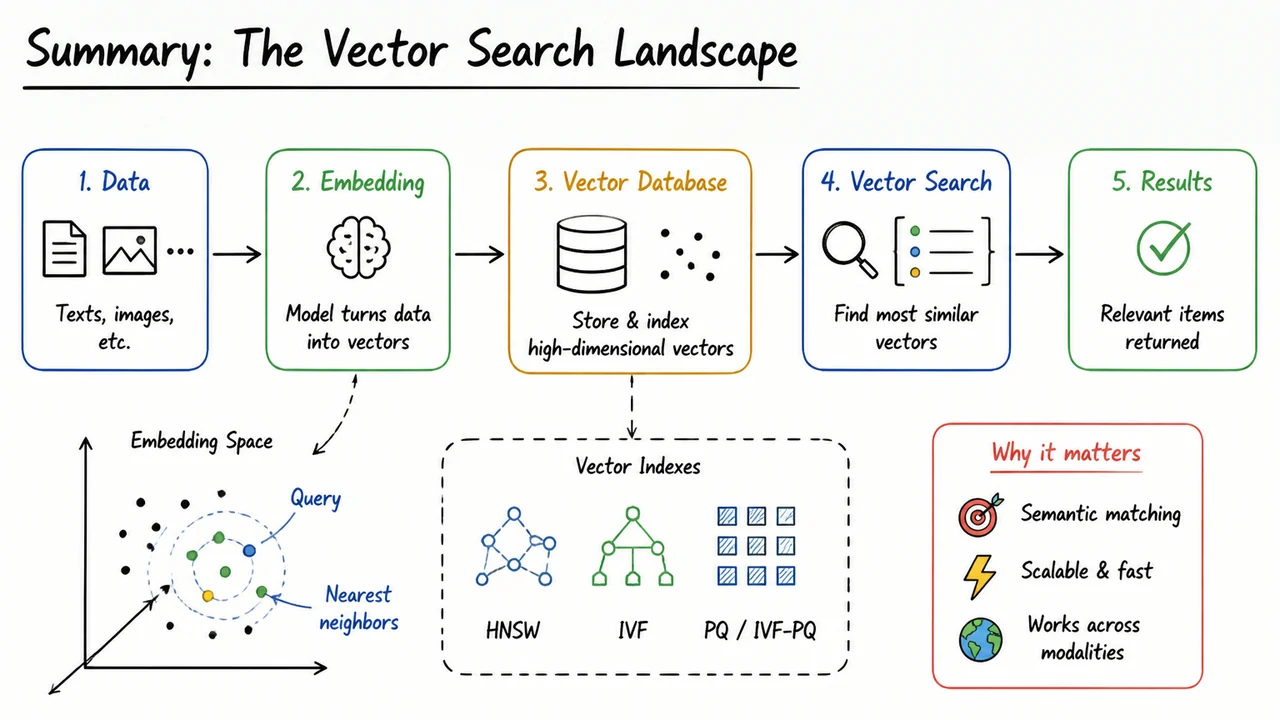
All of these threads are woven together in the diagram below, which maps the vector search landscape from representation to retrieval. It uses clear, sketched regions to separate embedding training, ANN theory, index families, and system architecture, with arrows showing how each component feeds into the next. The labels are concise—"Contrastive Learning", "J‑L Lemma", "IVF/PQ", "HNSW", "Vector DB Layer" — but each one condenses an entire design philosophy that we have now explored in detail. Together they form a minimalist map of a complex but increasingly essential subfield of machine learning infrastructure.