Imagine watching a reinforcement learning agent master an Atari game. After tens of millions of frantic frames — button presses, missed shots, pixel-level explosions — it eventually plays better than most humans. That’s the success story we hear about model‑free deep RL: a single network learns directly from raw pixels and rewards, turning a black‑box environment into a policy that acts. But behind the celebration lurks a sobering number. The canonical DQN (Deep Q‑Network) required ~200 million environment frames to surpass human‑level performance on a suite of Atari games. At 60 frames per second, that equates to roughly 38 days of continuous play. The agent does not share any of this experience across tasks; each new game forces the agent to start from scratch, burning another 200 million interactions just to rediscover the mechanics of paddles, bullets, or gravity.
This brute‑force requirement exposes the central weakness of model‑free RL: it treats the environment as a complete unknown and relies solely on trial‑and‑error to assemble a strategy. The agent’s mind has no internal representation of how the world behaves — no understanding that pushing right will move a paddle to the right, that a ball bouncing off a wall will reverse its trajectory, or that a specific enemy pattern repeats every few seconds. All such structural knowledge must be re‑extracted from raw data every time, leading to catastrophic sample inefficiency.
Contrast this with a human player. Give a person a new Atari game she has never seen, and within minutes — perhaps dozens to a few hundred actions — she grasps the objective, learns the basic controls, and starts achieving non‑trivial scores. She does not need to die ten thousand times to figure out that touching a monster is bad; a few observations and a quick mental model of cause and effect suffice. This ability to generalize from a handful of examples is often called one‑shot or few‑shot adaptation, and it is a hallmark of biological intelligence. The human brain constructs a compact internal simulator of the game’s dynamics, allowing her to plan tentative moves, predict outcomes, and transfer concepts like “avoid moving obstacles” or “collect shiny objects” instantly.
In reinforcement learning, we quantify this discrepancy with sample efficiency: the number of environmental interactions required to reach a target performance threshold. For many real‑world applications — robotics, autonomous driving, medical treatment design — collecting millions of trials is prohibitively expensive or dangerous. A robot cannot keep falling down thousands of times just to learn to stand. Therefore, the gulf between human‑level sample efficiency and model‑free RL’s hunger for data motivates a fundamental shift in how we build agents. The core insight is that an agent equipped with a learned model of its world can drastically reduce the interactions needed, because it can rehearse, plan, and “dream” inside its own simulator instead of always querying the real environment.
The problem with model‑free RL is not just the sheer volume of data; it’s the lack of transfer. Without an internal dynamics model, each new task demands massive re‑exploration, even if it shares underlying physics with a previously mastered task. The agent cannot say, “This game looks like the last one but with different colors; I’ll reuse my mental model of gravity and collision.” Every pattern must be rediscovered. A learned world model, on the other hand, captures the invariant causal structure of the environment, enabling rapid adaptation and, as we will see later, allowing the agent to compress experiences, generate imagined rollouts, and train a compact policy entirely within its own mind.
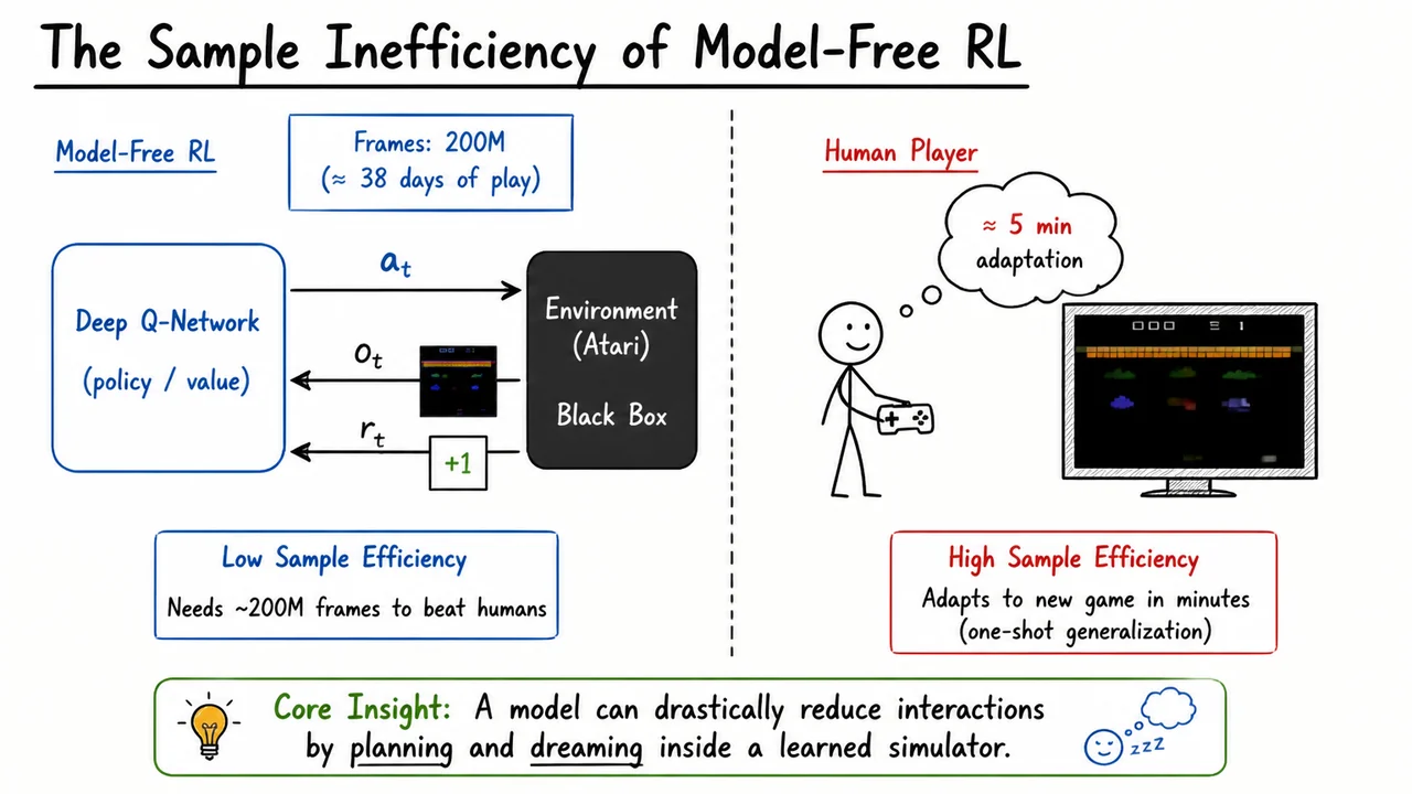
The visual below distills this contrast into a single glance. On the left, it draws a schematic of the model‑free loop: a labeled box for a Deep Q‑Network outputs an action into an opaque black‑box “Environment (Atari)”, which returns the next observation and a scalar reward . A stark counter reads “Frames: 200M,” and inside the agent’s box there is no internal structure beyond a generic “policy/value” node — a blind mapping from pixels to actions. On the right, the diagram shows a human figure beside a screen displaying a new, unfamiliar game; a thought bubble captures the rapid adaptation: “≈ 5 min adaptation.” The blue‑on‑red color scheme visually pits the slow, data‑guzzling model‑free approach against the fast, model‑rich human mind, making the argument for world models self‑evident.
This side‑by‑side layout immediately communicates why we need to move beyond model‑free methods. It hints at the solution: if we could replace the black‑box environment with a learned internal simulator, the agent could practice inside its own head and escape the tyranny of 200‑million‑frame trial‑and‑error. The rest of this lecture will show exactly how to build, train, and use such a dream‑capable world model.
The brute‑force approach of model‑free RL — learning a policy or value function entirely from live, high‑fidelity interaction — is extremely wasteful. Even the most sample‑efficient algorithms often require hundreds of thousands or millions of real environment steps to achieve competent behavior. This is not merely an engineering inconvenience; it fundamentally restricts reinforcement learning to domains where data is cheap or simulation is already perfect. The natural antidote is to give the agent the ability to build its own predictive simulator of the world. That shift, from experiencing to predicting, is the heart of model‑based reinforcement learning.
In model‑based RL, the agent learns an approximate world model of the environment’s dynamics. Rather than treating every transition as a black‑box surprise, the agent maintains two learned functions:
These approximations are trained on the same real interaction data the agent collects, but once they are reasonably accurate, they unlock a completely different mode of operation. The agent can now plan by unrolling its model many steps ahead, exploring imagined trajectories that never touch the true environment. Policy training can be carried out entirely inside this synthetic world, using virtually unlimited dream rollouts.
The sample efficiency advantage is stark. A single real transition can be used to train the model, and thereafter the model can generate thousands of simulated successor transitions at zero additional cost in real interactions. This decouples the agent’s learning from the environment’s interaction budget. Even crude early models can provide useful synthetic data that accelerates exploration or stabilizes policy updates. It is not an overstatement to say that model‑based methods trade real‑world samples for computation, a currency that modern hardware supplies in abundance.
Yet this elegant solution introduces a critical and insidious risk: model bias. Every transition model is an imperfect approximation of the true dynamics. When the agent plans or trains on imagined rollouts, small errors in a single‑step prediction compound multiplicatively over the rollout horizon. After a handful of imagined steps, the synthetic observations can drift into regions of state space that are either physically impossible or never encountered during real interaction. The policy, trained relentlessly on these flawed fantasies, learns to exploit the inaccuracies of the model rather than mastering the actual task. In the worst case, the agent discovers a policy that scores perfectly in the learned simulator but fails completely in reality. Controlling this compounding error is the central challenge of model‑based RL, and it is a theme that will recur in every section that follows.
The rest of this lecture takes model‑based RL into the high‑dimensional visual domain. Instead of trying to predict raw pixels directly — a task that is both computationally prohibitive and prone to catastrophic error accumulation — we will learn a compressed, latent world model. This enables a practical pipeline where a generative model (VAE) distills images into low‑dimensional features, a recurrent network (MDN‑RNN) models the stochastic dynamics of the latent state, and a compact controller learns to act within that imagined latent space. But before we dive into that architecture, it is worth pausing to visualize the qualitative difference between model‑free and model‑based loops.
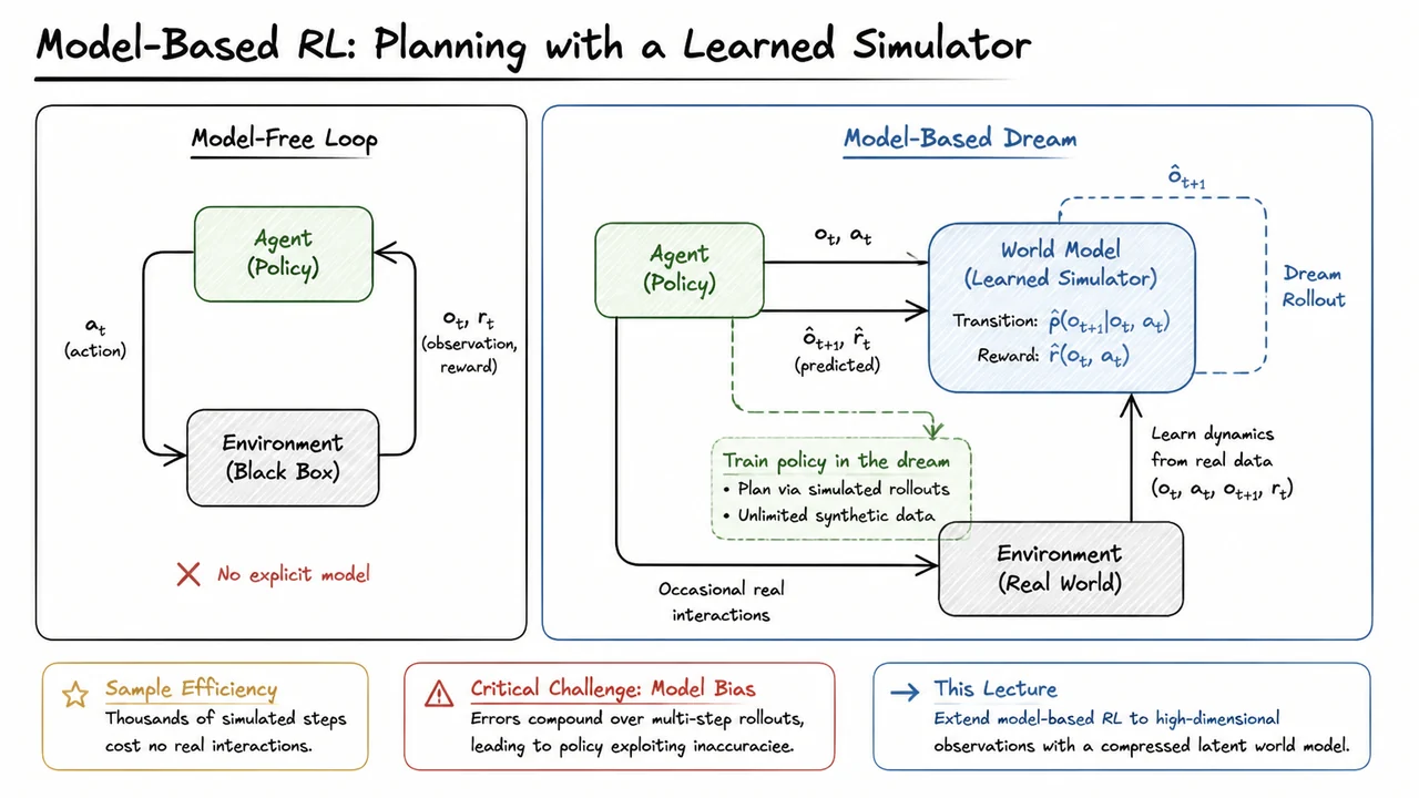
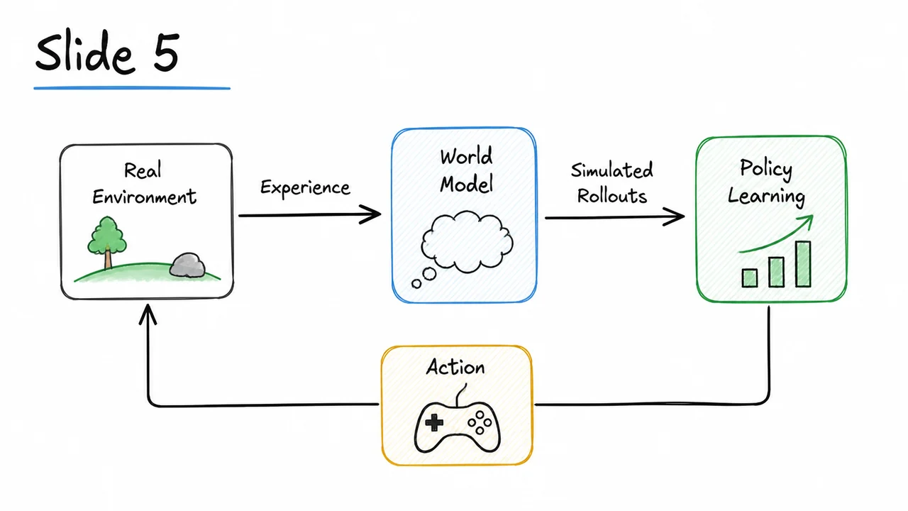
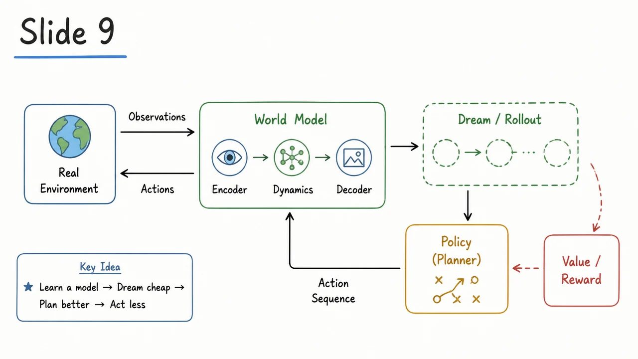
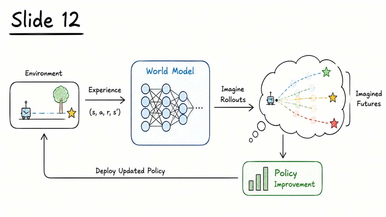
The accompanying diagram makes the contrast immediately tangible. On the left, the familiar Model‑Free Loop shows an agent that interacts directly with a gray, opaque environment: actions are emitted, observations and rewards are received, and all learning must occur within that closed loop. The right panel — the Model‑Based Dream — introduces a blue World Model block that sits between the agent and the environment. The model first digests real transitions to learn and ; then a dashed Dream Rollout loop takes over. Instead of querying the real environment, the model re‑feeds its own predicted next observation (along with actions) into itself, generating an unlimited stream of synthetic data. The green Agent (Policy) block can now be trained using these dream trajectories, completely decoupled from the grey real world. The dashed blue arrow loop is the visual essence of the idea: learning to dream as a replacement for constantly asking reality for one more expensive step. This architectural split — real data for model training, synthetic data for policy training — is what makes sample efficiency possible, while the accumulating error in the dashed loop is the silent threat we must now learn to contain.
Having established that model-based reinforcement learning can plan with a learned simulator, a natural question arises: can we directly apply these ideas to environments with high-dimensional observations, like raw pixels from a racing game? In theory, yes – we could train a transition model that predicts the next frame of pixels. In practice, raw pixel prediction is both computationally expensive and unreliable: small errors accumulate, the model often blurs details or produces implausible hallucinations, and planning through such a flawed model quickly diverges. The Dream Hypothesis, introduced by Ha and Schmidhuber (2018), elegantly sidesteps this problem by separating perception and dynamics from the decision-making policy, and training the latter entirely inside a learned dream.
The core insight is to decompose the agent into a large, pre-trainable World Model and a compact Controller. The world model’s job is to compress high-dimensional observations into compact, meaningful latent representations and to learn the stochastic dynamics that govern transitions between these latent states. The controller, on the other hand, is a small, focused network that takes latent features (and possibly some recurrence) as input and outputs actions – it never sees a raw pixel. Crucially, the controller is trained exclusively inside the world model’s imagination, not by interacting with the real environment. This architecture shifts the heavy computational burden to an offline pre-training phase, where the world model learns to dream plausible futures from unlabeled experience, while the controller remains lean and can be optimized efficiently with only simulated rollouts.
Two components form the World Model. The first is a Variational Autoencoder (VAE) that maps each high-dimensional observation (e.g., a screen frame) to a low-dimensional latent code . The VAE is trained to reconstruct the original observation, encouraging to capture essential structure while discarding irrelevant pixel-level noise. The second component is a Mixture Density Network combined with a Recurrent Neural Network (MDN-RNN). This network takes the current latent state , the action , and an internal hidden state that summarizes the history, and outputs the parameters of a Gaussian mixture distribution over the next latent state and reward:
The MDN-RNN thus captures the stochastic dynamics and intrinsic uncertainty of the environment in the compact latent space. Because the VAE decoder is still available, the world model can – if desired – render a dream observation:
However, the controller does not need to see these pixel reconstructions; it only relies on the latent codes and rewards.
Pre-training of the world model is remarkably flexible. The VAE and MDN-RNN can be trained on unlabeled random rollouts, for example from a random agent or even from a human demonstrator, without any reward maximization in mind. This means we can collect a dataset of transitions purely for the purpose of learning to imagine, and the world model learns to hallucinate plausible environment dynamics independent of any specific task. Once trained, the world model can generate an endless stream of “dreamed” rollouts: starting from an initial latent state and hidden state , the model repeatedly samples and conditioned on the current action. These dreamed trajectories contain all the information the controller needs: latent states and rewards.
Training the controller inside the dream then becomes a black-box optimization problem. Because the controller operates on a low-dimensional latent input and the dream dynamics are differentiable in principle, one could use gradient-based methods. The original World Models paper, however, employed Evolution Strategies (CMA-ES) to optimize the weights of a compact linear policy directly for cumulative dreamed reward, completely circumventing the need to backpropagate through time or through the world model. This separation allows the controller to be extremely small, sometimes containing only a few hundred parameters, and yet achieve competitive performance when deployed in the real environment.
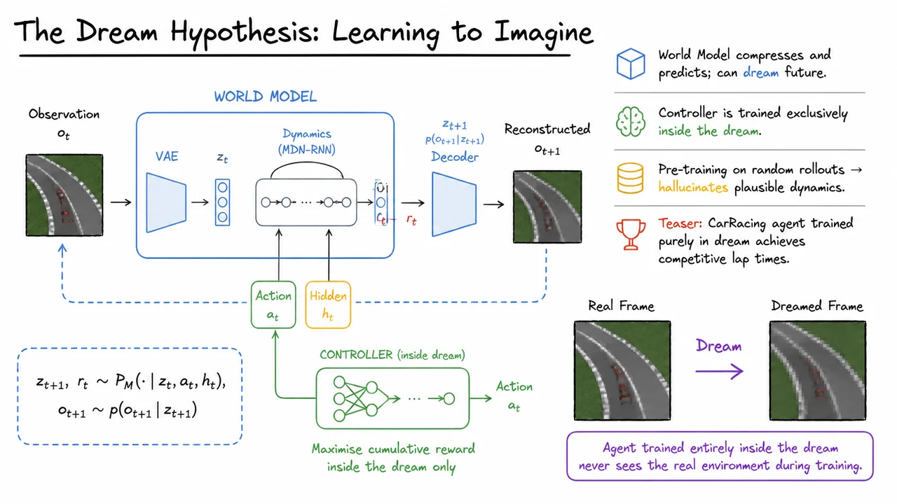
A remarkable demonstration of the dream hypothesis comes from the CarRacing environment. After pre-training the world model on random rollouts, an agent was trained entirely inside the dream, evaluating thousands of simulated episodes without ever seeing a real frame during the controller’s training. When transferred to the real game, this purely dreamed-up policy achieved competitive lap times, validating that the hallucinated environment was sufficiently realistic. The visual below juxtaposes a real frame from CarRacing on the left with a dream-generated frame on the right, connected by an arrow labeled “Dream”. The dream image, though slightly blurry, retains the structure of the winding road, the red car, and the surrounding grass – enough for a controller to learn effective steering and acceleration. A caption reinforces the key claim: the agent trained entirely inside the dream never sees the real environment during training. This image serves as both a conceptual summary and a piece of empirical evidence that dreaming can replace real interaction for policy learning, provided the world model is capable of faithful reconstruction and dynamics modeling. In the following sections, we will formalize the objective functions for the VAE, the MDN-RNN, and the controller, and examine how later frameworks like Dreamer and MuZero built upon this dream hypothesis.
The leap from dreaming to a rigorous problem statement requires us to ground the conversation in the formal language of reinforcement learning. In model‑free deep RL, an agent learns a policy that directly maps high‑dimensional observations to actions by sampling millions of environment transitions. This is profoundly sample‑inefficient: every pixel of every frame is processed essentially as raw data, and no internal model of the world ever emerges. The agent cannot mentally simulate “what would happen if” without actually executing the action in the real environment. The dream hypothesis (Ha and Schmidhuber, 2018) proposes a deceptively simple alternative: learn a compressed generative model of the environment, then train a compact policy entirely inside that learned dream. To make this precise, we need a shared notation and a clear decomposition of the learning pipeline.
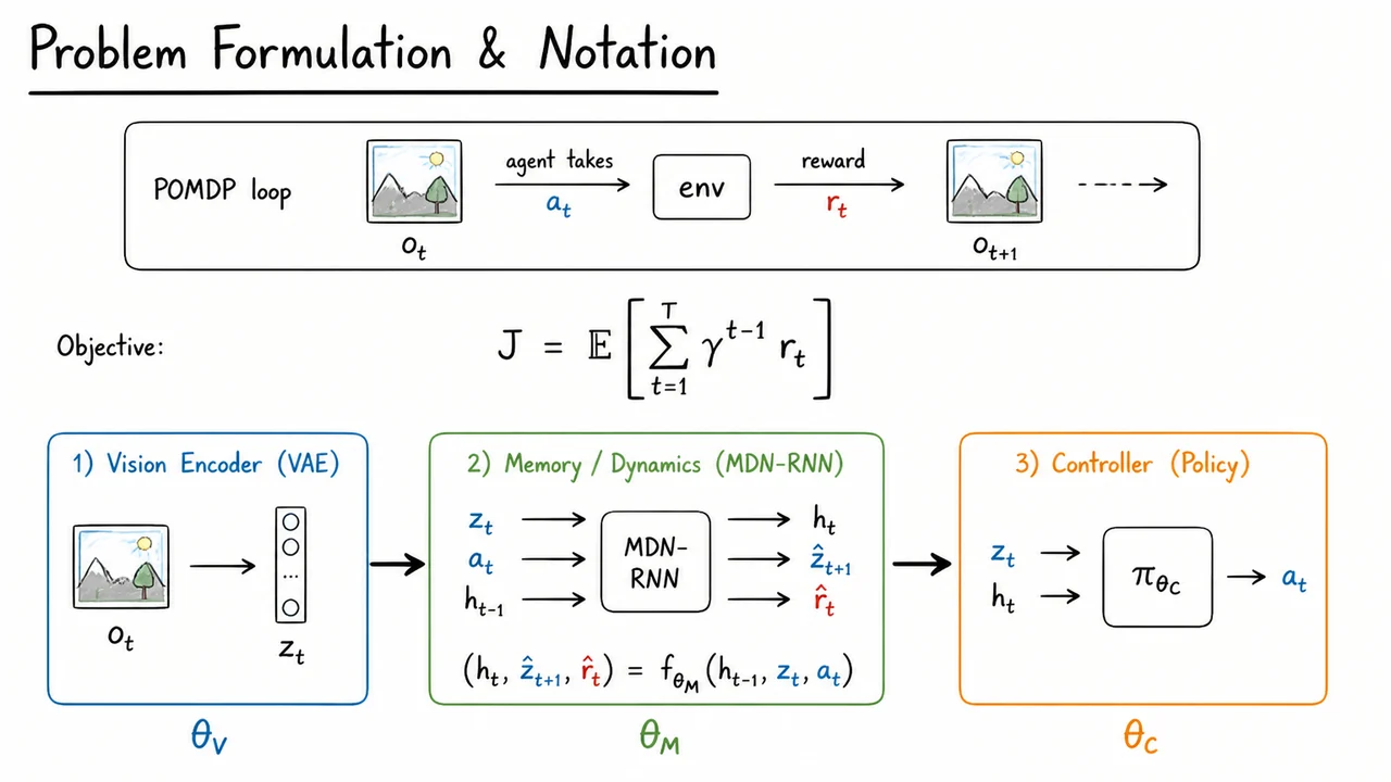
We treat the environment as a partially observable Markov decision process (POMDP) with high‑dimensional observations. At each discrete time step , the agent receives an observation – for instance, an RGB frame from a video game – and must select an action . The environment then returns a scalar reward and transitions to the next observation . The true underlying state of the environment (the exact physics, object positions, velocities) is not directly visible; the agent sees only the pixel matrix. The objective, as in standard RL, is to maximize the expected cumulative discounted reward from the start to a terminal time :
where is the discount factor. When is a high‑dimensional sensory stream, directly optimizing via model‑free methods like policy gradients or Q‑learning demands an enormous number of real interactions because the policy must implicitly learn a perception system, a state representation, and a value function all at once.
The World Models blueprint circumvents this by factorizing the problem into three learned modules, each with its own parameter set and training schedule. The first module, a vision encoder (typically a variational auto‑encoder, VAE), maps the raw observation to a compact latent vector . This step discards irrelevant detail while preserving the information needed to predict future frames. The VAE is trained offline on a dataset of collected frames, learning parameters that define both the encoder and the decoder (the decoder is used only to verify reconstruction quality and is not part of the dreaming loop).
The second module is a memory‑based dynamics model. Because the environment is partially observable, the latent vector alone may not contain enough information to predict the future. The model therefore maintains a recurrent hidden state that summarises the entire history . The dynamics model, parametrised by , is a Mixture Density Network combined with an RNN (MDN‑RNN). At each step it takes the previous hidden state , the current latent , and the action to produce the new hidden state, a prediction of the next latent , and a prediction of the reward :
The MDN component outputs a Gaussian mixture distribution over , capturing the stochasticity of real‑world transitions and making the dreamed rollouts more robust. The reward prediction is typically a single scalar head. Training the dynamics model requires sequences of collected by running a random policy or the current controller in the real environment; the MDN‑RNN is then optimised by maximum likelihood.
The third module is the controller, parametrised by . It is a simple policy – in the original work, often just a linear model – that maps the concatenation of the latent state and the memory state directly to the action: . Crucially, the controller is not trained on real environment trajectories. Instead, it is optimised entirely inside the learned dream: the world model (VAE + MDN‑RNN) is frozen, and the controller is tasked with maximising the cumulative dreamt reward. Because the world model is fully differentiable only with respect to the controller’s inputs, evolution strategies (e.g., CMA‑ES) or other black‑box optimisation methods are used to update without requiring backpropagation through the whole model.
This three‑way decomposition – for perception, for dynamics and memory, for behaviour – is the conceptual engine behind the approach. It separates representation learning from forward prediction and from decision making, allowing each component to be trained with a method suited to its role. The VAE learns a compressed space, the MDN‑RNN learns to roll out and evaluate imagined trajectories, and the controller learns a task‑specific policy without ever seeing a real pixel again after the initial data‑gathering phase. By dreaming, the agent can simulate thousands of episodes per second, radically reducing sample complexity.
The visual that accompanies this section distills the full problem formulation into a single, glanceable architecture. It begins with a narrow box representing the raw POMDP loop – the flow of , , and – and places the central objective prominently below it. Then, in a horizontal row, three colour‑coded modules appear: a blue encoder compressing into ; a green memory‑dynamics block taking , , and to produce , , and ; and an orange controller mapping to the next action. Beneath each module, the corresponding parameter symbols , , and are shown, reinforcing that the world model is not one monolithic network but a carefully composed ensemble. This diagrammatic summary makes the abstract notation concrete: the reader can see at a glance how perception, imagination, and action are welded together into a system that learns to dream before it learns to act.
The previous section framed reinforcement learning as a sequential decision problem—an agent interacting with an environment to maximize long‑term reward—and established the notation for observations, actions, states, and trajectories. In principle, we could solve such problems with model‑free algorithms that directly map pixels to actions through deep networks, and indeed spectacular results have been achieved this way. Yet anyone who has trained a DQN or PPO agent on a visually rich environment knows the pain: millions of environment steps, painfully slow wall‑clock times, and fragile policies that collapse when the reward signal becomes sparse or deceptive. The root cause is sample inefficiency. Model‑free methods treat the world as a black‑box oracle that must be queried for every single scrap of experience, and they rarely share that experience across tasks or can re‑use the underlying dynamics for anything else.
The world models approach turns this on its head. Instead of discarding the environment after each interaction, we learn a compressed, predictive model of it. The idea is elegant: the agent first builds an internal “dream simulator” of the environment’s dynamics in a compact latent space, and then trains its policy almost entirely inside that dream. The real environment is still needed, but only occasionally, to ground the dream in reality. In this way, we replace expensive physical interaction with cheap, parallelizable simulated rollouts—while preserving the essential causal structure of the problem.
To see how this is possible, consider what an agent truly needs from a high‑dimensional observation like a game frame. A 96×96×3 image contains over 27,000 numbers, but the information that matters for decision‑making—the position of the car, the curve ahead, the velocity—likely lives on a manifold of much lower dimension. If we can learn a mapping that compresses each raw observation into a small latent vector which faithfully captures the task‑relevant state, we can then model the environment’s dynamics using only these latent codes. Formally, we want a generative model that captures and a recognition model (encoder) that approximates ; that is precisely what a Variational Auto‑Encoder provides.
But compression alone is not enough. We also need to know how evolves in response to actions. If we attempted to model the transition with a deterministic function, we would quickly be disappointed: the real world, and even many simulated environments, contain stochastic elements (e.g. random track textures, friction variability, or noisy actuation). The next latent state is better described by a mixture of Gaussians, whose parameters depend on the current latent state, the action, and also on a hidden memory state that accumulates information over time. An MDN‑RNN (Mixture Density Network combined with a recurrent neural network) fits this role naturally: the RNN maintains a deterministic hidden state that integrates past experience, and at each step the MDN head outputs the parameters of a Gaussian mixture that models the distribution of and possibly the reward . The model is trained by maximizing the likelihood of real trajectories observed so far.
With the VAE compressing observations and the MDN‑RNN predicting future latent encodings, we have the core of a world model. The third component is a compact controller that maps the concatenation directly to an action . Because the latent representation is small and the dynamics model is differentiable (or can be treated as a black‑box simulator), we can train the controller without back‑propagating through the visual encoder. The original Ha and Schmidhuber paper used evolution strategies (ES) for this final step: they perturb the controller’s weight vector, run many imagined rollouts inside the world model, and keep perturbations that lead to higher total dreamt reward. That strategy is simple, parallelizes across CPU cores, and avoids credit‑assignment issues that often plague long imagined trajectories.
This separation into three trainable modules—a visual encoder, a latent‑space dynamics model, and a controller—is what gives the world model its power and its name. Once the VAE and MDN‑RNN have been trained on a modest set of real transitions, the agent can dream: it starts from the latent encoding of a true frame and then, for hundreds of steps, feeds its own predicted back to the RNN, collecting simulated rewards, all without ever rendering a pixel or touching the real environment. Training the controller inside this dream is not only faster; it also decouples the policy search from the slow, serial process of real‑world interaction.
The visual below captures this entire pipeline in one coherent diagram. It shows the three modules—VAE, MDN‑RNN, and controller—connected by arrows that trace the flow of information. On the left, a high‑dimensional observation passes through the VAE encoder to become a compact latent . That latent, together with the previous hidden state and action , feeds into the MDN‑RNN, which updates its hidden state to and predicts the parameters of a mixture distribution over the next latent state and, optionally, the reward. The controller takes the concatenation and outputs the next action . A dashed loop indicates the “dream” mode: the model can run autonomously by replacing the real with a sample from the MDN‑RNN’s predicted distribution, enabling long simulated rollouts. Hand‑drawn annotations and muted colors—blue for the VAE, amber for the MDN‑RNN, green for the controller—help the reader instantly separate responsibilities while seeing how they cooperate to form the full world model.
Reinforcement learning agents that operate directly on raw sensory inputs—pixels from a game frame, for example—face a punishing sample inefficiency. Learning a value function or a policy from high-dimensional observations without any prior structure can require millions of environment steps, most of which are spent rediscovering the same basic visual features. The World Models framework attacks this problem by decomposing the agent into a large world model that learns a compressed, predictive representation of the environment, and a compact controller that acts within that learned representation. The heavy lifting is done by the world model, which is trained offline and can even “dream” simulated experience, relieving the controller from having to reconstruct the world from scratch every time it makes a decision.
The first pillar of this world model is a vision module whose job is brutally simple: take a high-dimensional observation (say, a 64×64 RGB frame) and compress it into a low-dimensional latent vector that preserves only the information relevant to solving the task. If this compression works well, then all downstream learning—predicting future latents, training the policy—happens in a space that is orders of magnitude smaller and where geometric relationships are much easier to model. The chosen tool is a Variational Autoencoder (VAE), which provides a principled probabilistic framework for learning such a compact latent code.
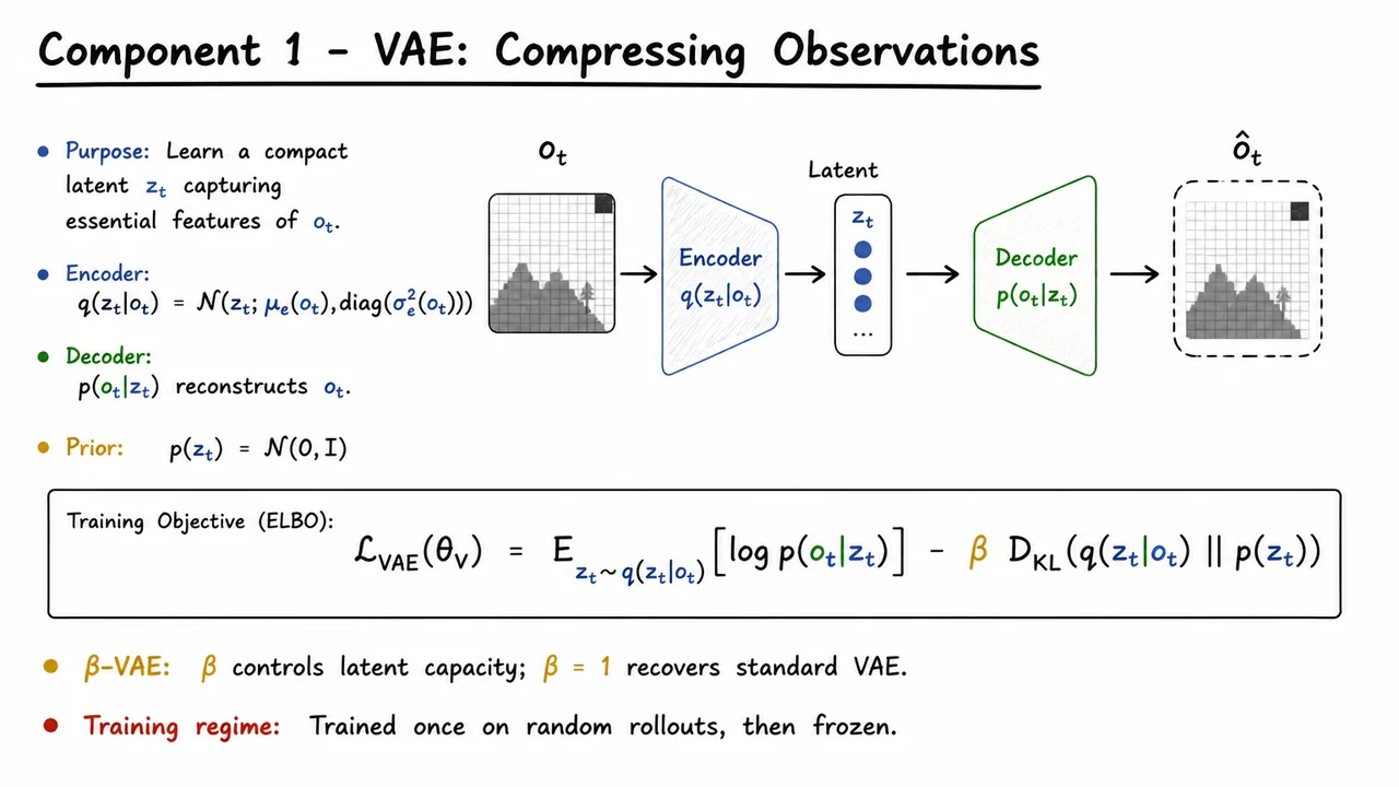
A VAE models the generative process that produces observations from latent codes, together with an approximate posterior that acts as an encoder. In the World Models implementation, both the encoder and decoder are neural networks parameterized by . The encoder outputs the parameters of a diagonal Gaussian distribution over the latent variable: Sampling from this distribution via the reparameterization trick yields a stochastic that can be passed through the decoder to reconstruct the observation. The choice of a stochastic encoding is essential: it provides a natural way to inject noise and uncertainty, and it regularizes the latent space so that nearby points decode to visually similar frames, which in turn helps the next component—the dynamics model—operate smoothly.
To train the VAE, we maximize the Evidence Lower Bound (ELBO) on the log-likelihood of the observed data, but with a crucial modification—a scalar that scales the KL divergence term: The first term is the reconstruction log-likelihood; for pixel data it is often a Gaussian likelihood with fixed variance (equivalent to an L2 loss) or a Bernoulli likelihood (binary cross-entropy). The second term pulls the approximate posterior toward the prior . When we recover the standard VAE; larger values of push the model toward a -VAE that encourages disentangled factors in the latent space, and smaller values trade off reconstruction fidelity for a weaker prior penalty. In the World Models paper, is tuned to balance latent capacity against reconstruction quality, though the primary aim is still to get a compact, usable representation for the dynamics model rather than perfectly disentangled features.
Importantly, the VAE is trained once on a dataset of observations collected by a random agent interacting with the environment, and then its weights are frozen. The encoder becomes a fixed perceptual module; every subsequent step of world-model learning or controller optimization simply calls the encoder to produce from the current . This design choice has profound implications. On the positive side, it decouples representation learning from policy learning, making training far more efficient—the controller never has to worry about high-dimensional vision. On the negative side, the VAE’s world representation is only as good as the random data it has seen. If the random rollouts never visit parts of the state space that a good policy would later require, the representation will have blind spots. Realigning the world model later or updating the VAE online are natural extensions to address this.
What goes into the latent ? The VAE is encouraged to discard pixel-level details that are irrelevant for control—like background textures, sky gradients, or tiny fluctuations—while retaining crucial spatial structure: the position of the car, road boundaries, obstacles, and their relative velocities. Because the VAE is probabilistic, the latent itself becomes a compact, smooth summary that already starts to abstract away the raw sensory stream. The visual that follows consolidates this whole pipeline: it shows the encoder mapping to a mean and variance, the sampling step to obtain , and the decoder reconstructing . The central display equation for the ELBO encapsulates the training objective, and the parameter is highlighted to remind us that its weight controls the trade‑off between faithful reconstruction and a well‑shaped latent prior. With the VAE in place, we can now turn to the second component—a dynamics model that learns to predict the next latent state given and the action —and begin to “dream” in this compressed space.
Having compressed each high-dimensional frame into a compact latent representation with the VAE, we now face a deeper challenge: the environment doesn’t just deliver a static picture—it evolves in response to actions, often in stochastic ways. Model-free RL learns this evolution implicitly through value functions or policy gradients, but it requires an immense number of environment interactions because it must rediscover the consequences of actions from scratch every few updates. The World Models architecture addresses this by learning an explicit dynamics model in the latent space that can be used to simulate trajectories without ever rendering pixels. This is where the Memory Module, the MDN-RNN, becomes essential.
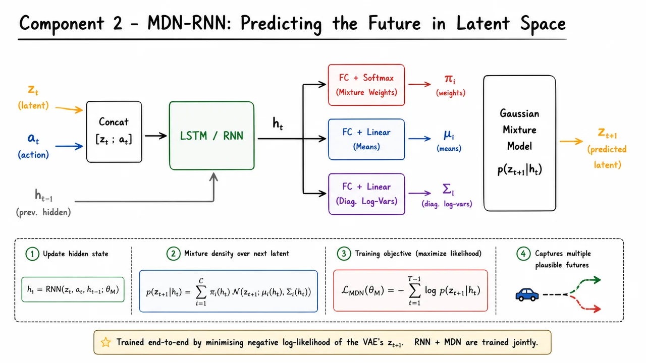
At its core, the MDN-RNN is a recurrent neural network that takes the current latent state and action , along with its own previous hidden state , and produces a new hidden state . That hidden state serves two purposes: it acts as a compressed memory of the episode history so far, and it parameterizes a predictive distribution over the next latent state . The recurrence is crucial because the true future of an environment depends not just on the current observation and action but on unobserved aspects like velocity, momentum, or hidden intentions of other agents—information that can only be accumulated over time. The RNN (typically an LSTM or GRU) ingests the concatenation of and , along with , and outputs , which becomes the internal belief state for the next step.
What makes the MDN-RNN special is that it does not output a single deterministic prediction for . Instead, it models the environment’s stochasticity with a mixture density—a weighted sum of Gaussian distributions whose parameters are functions of the hidden state. The output layer transforms into three sets of vectors: the mixing coefficients , the means , and (typically diagonal) covariance matrices for each of mixture components. Then the probability density of the actual next latent state is given by
The softmax over the ensures these weights sum to one, while the means and variances give location and spread of each component. This construction is a natural choice for world models because many real-world transitions are multi-modal: from the same state and action, several distinct futures might be possible. For example, when the agent drives a car toward an intersection, the next state could be a left turn or a right turn, not a smooth average of both. A single Gaussian would place its mass in the middle, predicting an impossible blend; the mixture can assign separate peaks to each plausible outcome.
Training the MDN-RNN is a straightforward supervised learning problem: we collect a large dataset of trajectories by running a random or preliminary policy in the environment, encode every frame with the frozen VAE to obtain the sequence of latent vectors , and then optimize the network parameters to maximize the likelihood of each actual next latent state given the history. This translates into minimizing the negative log-likelihood over all time steps:
Notice that the targets are the VAE’s compressed representations—real vectors, not discrete tokens—so the mixture density deals with continuous latents. Because the VAE itself is stochastic, the latents already carry some noise, and the MDN learns to absorb that uncertainty into its predictions. A common practical choice is to use diagonal covariances , which keeps the number of parameters manageable and makes the log-density calculation efficient, while the multiple components still capture complex shapes through overlap.
An important subtlety is that the RNN and the mixture-density heads are trained jointly end-to-end. The hidden state is not just a summary of past observations; it is shaped by the learning signal that flows back from the prediction errors on future latent states. This means the network learns to extract exactly the temporal features that are useful for forecasting, often discovering dynamics-related invariants like velocity or acceleration without any explicit supervision. Once trained, the MDN-RNN can simulate in latent space: at each step, we sample a from the predicted mixture, feed it back as the next input together with the action, and continue the dream.
The visual below consolidates this architecture into a single flowing diagram. On the left, three incoming signals— (the current VAE latent, colored orange), (action, blue), and the recurrent hidden state (gray)—enter a central LSTM/RNN block, which outputs the updated . From that hidden vector, three parallel fully connected layers branch out: a softmax layer producing the mixture weights , a linear layer producing the component means , and another layer producing the (diagonal) log-variances . These three groups of parameters feed into a rounded box labeled “Gaussian Mixture Model ”, from which an arrow points to the predicted next latent . Beneath the diagram, a concise caption reminds us that the whole module is trained by minimizing the negative log-likelihood of the actual VAE latent from recorded rollouts. The diagram matches exactly the step-by-step computation we’ve just described, making the interplay between recurrence, mixture modeling, and training signal immediately apparent.
Having designed an RNN that can forecast future latent states, we hit a more fundamental question: how do we get from raw pixels to the compact, information-dense representations that the dynamics model needs? World Models answers this with a variational autoencoder (VAE), a generative model trained to compress high-dimensional observations into a low-dimensional latent space while retaining enough detail to reconstruct the original frame. The VAE’s objective is not a simple reconstruction loss but a principled lower bound on the log-marginal likelihood of the data, a derivation that sits at the heart of modern latent-variable modeling.
We begin by writing the marginal likelihood of an observation under a latent variable model with prior and likelihood . Dropping the time index for clarity, the log-marginal is
The integral over the latent space is generally intractable—we cannot enumerate all configurations for a high-dimensional image. The standard trick is to introduce an approximate posterior distribution , often called the encoder, and use it to rewrite the log-likelihood. By adding and subtracting the KL divergence between and the true posterior , we obtain
Since the KL divergence from the approximate to the true posterior is always non‑negative, dropping it yields a lower bound—the Evidence Lower Bound (ELBO):
This inequality crystallizes the VAE’s learning problem. The first term, the expected log-likelihood under the encoder’s samples, pushes the decoder to faithfully reconstruct the observation—for images, it boils down to per‑pixel Gaussian log-likelihood (MSE) or Bernoulli cross‑entropy. The second term, the KL divergence between the encoder’s output distribution and the prior , acts as a regularizer that pulls the latent representations toward a simple distribution, typically a standard Gaussian. The bound is tight exactly when equals the true posterior, so optimizing the ELBO encourages both accurate reconstruction and a well-structured latent space.
In practice, we often use a -VAE, where a coefficient scales the KL term:
When we recover the standard ELBO. Increasing enforces a stronger bottleneck, which can improve disentanglement of latent factors at the cost of reconstruction fidelity. For World Models, a moderate helps keep the latent codes compact and stationary, an ideal substrate for the MDN‑RNN to model over time.
A huge practical advantage of the VAE objective is that the KL term has a simple closed form under Gaussian assumptions. We choose the prior and let the encoder output the mean and variance for each dimension of a diagonal‑covariance posterior . Then the KL divergence becomes
This formula is purely arithmetic, so the loss is differentiable and cheap to compute. The reconstruction term is approximated by drawing one or more samples and using the reparameterization trick to backpropagate through the sampling step. The entire VAE is then trained end‑to‑end on a corpus of randomly collected frames from the environment—no reward signal needed.
The resulting latent vectors are low‑dimensional, continuous, and relatively smooth, which is exactly what the MDN‑RNN expects. Because the VAE is trained to maximise the ELBO, the latent space naturally captures the essential visual content while discarding irrelevant pixel‑level noise. This compression is what makes it possible to run the dynamics model thousands of steps ahead in a simulated dream, generating imagined trajectories that are both realistic and computationally cheap.
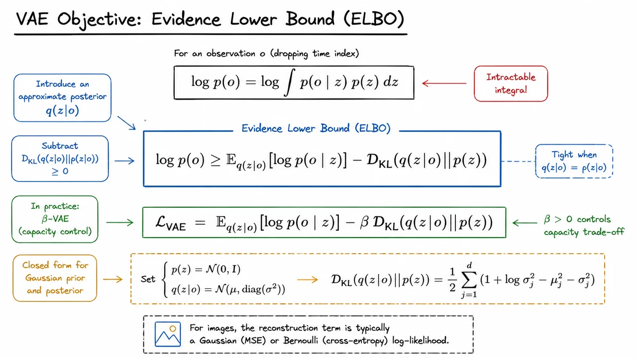
The visual below condenses these ideas into a clean reference. At the top, it shows the intractable marginal likelihood integral, emphasizing why a direct approach fails. A centered box then displays the core ELBO inequality: reconstruction expectation minus the KL penalty. Just beneath that, the -VAE loss is written out, underscoring the capacity‑control lever. Finally, the closed‑form KL divergence is given as a summation over dimensions, providing a ready‑to‑implement formula for the Gaussian case. In one glance, the diagram captures the mathematical flow from intractable marginal to trainable objective—a compact cheat sheet for the VAE component of World Models.
After mastering the VAE that squeezes high‑dimensional pixel frames into compact latent vectors, we face the next question: how does the world actually move from one state to the next? A static autoencoder gives us a useful alphabet, but efficient reinforcement learning requires a compressed forward model that can predict future latent states and rewards without looking at the raw sensory stream every time. This is precisely where the World Models architecture introduces its second component: a dynamics model trained entirely in the latent space of the VAE, typically realised as a Mixture Density Network combined with a recurrent neural network (MDN‑RNN).
The intuition is straightforward. An uncompressed environment frame (say, a image of a car racing track) contains far more detail than we need for planning. The VAE’s encoder already collapses this into a compact stochastic code . If we now observe a sequence of frames , we can compress each frame into a posterior sample and then train a recurrent network to predict the next latent state and the immediate reward given the history of previous latents and actions. Crucially, the MDN‑RNN does not output a single crisp prediction; it outputs a full probability distribution over the next latent vector. Since the latent space is itself stochastic (the VAE’s sampling step injects noise), a multimodal or heteroscedastic distribution is often needed. A Gaussian mixture model gives the network the flexibility to capture several plausible futures – for example, the car might continue straight or begin to swerve on a curve.
The training loss for the MDN‑RNN is simply the negative log‑likelihood of the observed next latent vector under the predicted mixture density, summed over time:
where is the RNN’s hidden state summarising previous latents and actions, are the mixing coefficients, and the network outputs all parameters of the Gaussians. A parallel head can predict the reward with a simple squared error or cross‑entropy loss if rewards are discretised. Because the dynamics model only sees the compressed latents and a continuous‑action input (e.g., steering and acceleration), it is orders of magnitude smaller than a pixel‑space predictor and can be rolled out for thousands of imagined steps in mere milliseconds.
Once the VAE and the MDN‑RNN are in place, we effectively possess a dream simulator: we can feed it an initial latent state and a sequence of actions, and it will hallucinate a chain of latent states and rewards. This dream world becomes the exclusive training ground for the controller – a small policy network that maps a latent state (and optionally the RNN hidden state ) directly to an action vector. Because the world model is fully differentiable or at least queryable at high speed, we can bypass traditional backpropagation‑through‑time limitations and instead use evolutionary optimisation, such as CMA‑ES (Covariance Matrix Adaptation Evolution Strategy), to search for controller weights that maximise the cumulative dream reward over many pseudo‑episodes.
The overall training pipeline thus consists of three stages that are repeated iteratively:
This decoupling is the core efficiency gain: the RL agent learns to imagine millions of steps per second, while only interacting with the true environment to occasionally update its world model. As a result, World Models achieved competitive scores on the CarRacing‑v0 benchmark using fewer than 1000 real episodes, a fraction of what model‑free methods require. The real genius is that the policy is never directly exposed to the original high‑dimensional observation; it lives entirely in the compact, abstract space learned by the VAE.
The visual below (or on the companion slide) consolidates this complete loop. It shows the three neural components – VAE encoder, MDN‑RNN, and controller – as hand‑sketched boxes arranged in a cycle: real frames enter the VAE to produce latents, the latents feed the MDN‑RNN which predicts future latents and rewards in a dream loop, and the controller receives latents from either the real world or the dream to output actions. Arrows indicate the flow of information and the distinct training signals (reconstruction loss for the VAE, next‑latent likelihood for the MDN‑RNN, and cumulative reward for the controller). By presenting the pipeline as a single diagrammatic snapshot rather than three separate slide bullets, the visual helps the learner instantly grasp how compression, dynamics, and policy co‑evolve in the World Models framework – a perfect summary before we turn to empirical results, failure modes, and the extensions that grew into Dreamer and MuZero.
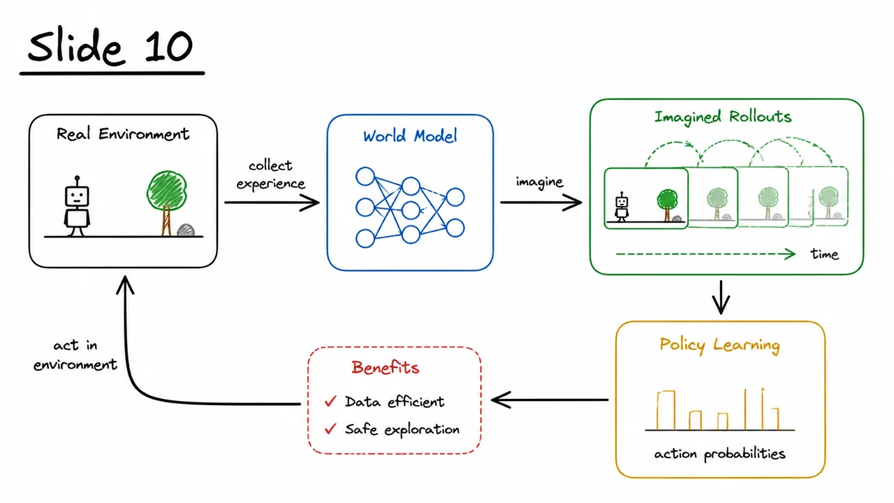
Model-free reinforcement learning—where an agent learns a policy or value function directly from raw interaction with an environment—has produced remarkable results on tasks from board games to robotic control. Yet its appetite for data is staggering. An agent that learns to play Atari games from pixels may require tens of millions of frames; a simulated robot learning to walk can consume days of compute. This sample inefficiency stems from a fundamental reliance on trial-and-error in the high-dimensional, noisy space of sensor readings. Every new environment demands the agent to relearn even simple regularities—like the fact that objects persist when they leave the frame—from scratch through a deluge of episodes. The promise of world models is to break this dependency by giving the agent an internal, compressed imagination it can use to simulate experience, dramatically cutting the number of real interactions needed.
The core idea is simple and beautifully recursive: if we can learn a model that predicts how the world behaves given an action, then the agent can “dream” plausible futures and plan or train a policy inside its own mind. In the seminal World Models paper by Ha and Schmidhuber, this is achieved with three cooperating components: a Variational Autoencoder (VAE) that compresses high-dimensional observations (e.g., game frames) into a compact latent vector, a Mixture Density Network combined with a Recurrent Neural Network (MDN-RNN) that models the stochastic dynamics of the latent state over time, and a compact controller that maps the latent state and the RNN’s hidden state to actions. The controller is kept deliberately small—often a linear model or a shallow neural net—so that it can be trained efficiently, even with black-box optimization methods like Evolution Strategies (ES). The magic is that once the VAE and MDN-RNN are trained, the controller can be optimized entirely inside the learned “dream” world, requiring zero additional real experience.
Let’s unpack the compression step. When observations are high-dimensional, like 64×64 RGB images, it is hopeless to model raw pixel dynamics with enough fidelity to roll out realistic simulations. The VAE solves this by learning a probabilistic mapping from the observation space to a low-dimensional latent space that captures the essence of the scene. A VAE consists of an encoder network that outputs the parameters of a distribution (usually a diagonal Gaussian) and a decoder network that reconstructs the observation from a sample of that distribution . Training minimizes a loss with two antagonistic terms: a reconstruction loss that encourages faithful decoding, and a KL divergence that forces the latent distribution to be close to a simple prior —typically . This yields the evidence lower bound (ELBO):
where balances compression fidelity. By setting (a β-VAE), the model is pushed to learn more disentangled, robust latent representations that later benefit the dynamics model. In the CarRacing environment, this compresses an image into a vector of merely 32 or 64 numbers, preserving the track layout, car orientation, and relevant visual cues while discarding irrelevant pixel-level noise.
With a compact latent space in hand, the next challenge is capturing how the environment evolves. A deterministic model would be fragile because many real-world (and even simulated) dynamics are unpredictable: for instance, a car’s behavior on a curve may depend on subtle friction or random perturbations. The MDN-RNN addresses this by predicting a distribution over the next latent state given the current latent , the RNN’s hidden state , and the action . More precisely, the network outputs the parameters of a mixture of Gaussians—weights , means , and standard deviations —so that the conditional density is
The MDN-RNN is trained to maximize the log-likelihood of the observed sequence of latent states (produced by the frozen VAE encoder) given the actions. Additionally, it predicts the immediate reward from the same hidden representation, using a mean-squared error loss. This multi-task objective encourages the hidden state to accumulate information about the history that is useful for both state transition and reward prediction.
The stochasticity modelled by the mixture of Gaussians turns out to be crucial: it allows the agent to dream varied, plausible futures rather than a single deterministic hallucination, which in turn produces a controller that is robust to the sorts of surprises the real environment might throw at it.
Finally, the controller. Given that the VAE and MDN-RNN are pre-trained on rollouts from a random policy (or gradually improved upon), the controller learns to act purely inside the dream. It receives the latent state and the RNN hidden state and outputs the action . Because the input space is small and the dynamics are already captured by the RNN, the controller can be tiny—a single linear layer with a activation, for instance. Training this controller using Evolution Strategies (ES) is elegantly sample-efficient within the dream: we simply sample perturbations of the weight vector, run hallucinated rollouts with the MDN-RNN, and keep the weights that maximize cumulative reward. No backpropagation through time is required, and the method is trivially parallelizable. The result is an agent that can solve complex tasks like CarRacing with orders of magnitude fewer real environment steps compared to model-free baselines.
The visual below brings these three components together into a coherent pipeline. High-dimensional observations are funneled through the VAE’s encoder into a tiny latent code ; the MDN-RNN takes that code alongside its own hidden state and the action to predict the next and the reward; the controller, seeing only and , produces the next action. The entire loop—encode, predict, act—runs either on real frames or on dreamed ones, with the dashed boundary indicating the “world model” that isolates the agent from the expensive real environment. It shows how compression and learned stochastic dynamics become the engine of efficient reinforcement learning, a template that later works like Dreamer and MuZero would refine and extend. Keep this architecture in mind as we now dive into the specific VAE compression on CarRacing.
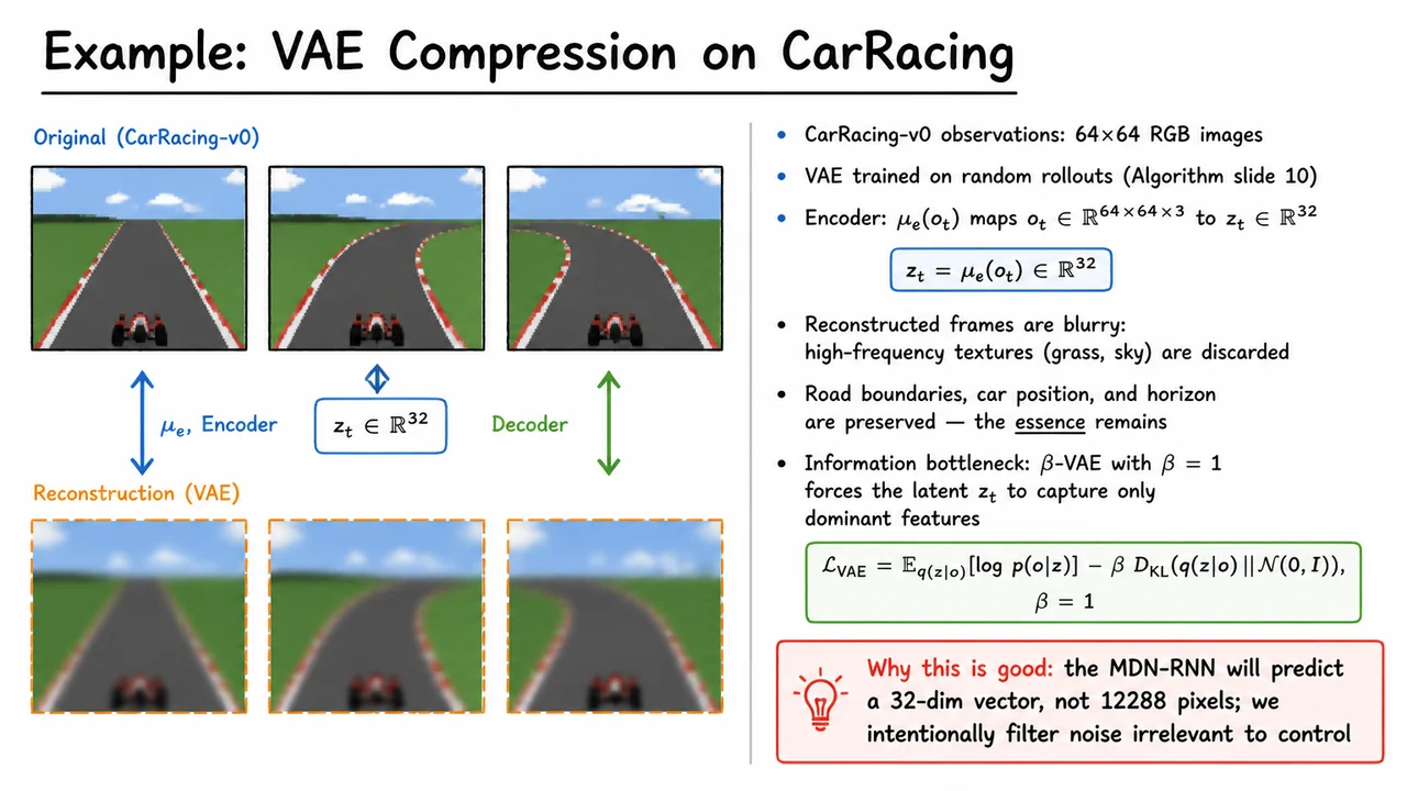
The previous section established the VAE as a principled way to learn a compact latent representation of high-dimensional observations. Now we see exactly how that abstraction earns its keep in the CarRacing-v0 domain, where every raw frame is a tensor—12,288 pixel values—that arrives at 60 Hz. If we naively fed those frames into a dynamics model, the sheer dimensionality would be prohibitively sample-inefficient, and much of the signal (grass textures, cloud patterns, minute colour fluctuations) carries no information about controlling the car. The first component of the World Models architecture therefore trains a -VAE as an information bottleneck that crushes this high-dimensional stream into a 32‑dimensional latent vector , discarding everything that does not help reconstruct the dominant scene structure.
Training the VAE does not require expert demonstrations or even a partially trained policy; it is performed entirely on random rollouts—frames collected by an agent taking uniformly sampled steering, acceleration, and brake actions. This is a critical design choice: the VAE never sees optimal driving, so it cannot accidentally encode a prior about “good” trajectories. Instead, it learns to represent the visual manifold of the environment itself, purely from the statistics of the image distribution. The loss function is the standard -VAE objective with :
The first term is the reconstruction log-likelihood—how well the decoder can recover the original frame from the sampled latent code. The second term is the KL divergence between the encoder’s distribution and a standard Gaussian prior, which acts as a regularizer that pushes the latent representation toward a smooth, continuous latent space. With (the classic VAE), this penalty is just strong enough to prevent the model from memorizing fine textures and pixel noise; the optimal solution balances accurate reconstruction of macroscopic geometry against a compact, well‑organized latent manifold.
The effect of this trade‑off becomes immediately visible in the reconstructions. When the VAE is asked to encode and decode a frame, the output is blurry: high‑frequency details like the rippling grass, the dithering of the sky gradient, and the tiny speckles of road texture are smoothed away. Yet the essence of the scene remains sharp: the road boundaries, the position of the horizon, the silhouette of the car, and the upcoming curves are all faithfully preserved. This is not a failure of the model but precisely the intended behaviour—the model has learned that those high‑frequency niceties are irrelevant for predicting itself under random jitter, and so the latent code devotes its limited 32 dimensions to capturing only the task‑relevant structure. In information‑theoretic terms, the VAE discards the “noise” that would otherwise drown the dynamics model in irrelevant variance.
Why is this blurring a feature, not a bug? The RNN that will learn the environment’s dynamics (the MDN‑RNN) now operates on vectors of 32 numbers instead of 12,288. Reducing the dimension by a factor of nearly 400 makes the prediction task dramatically easier, requiring orders of magnitude less data to converge. Moreover, the information bottleneck acts as an implicit denoising step: the dynamics model never sees the raw pixels, so it cannot inadvertently latch onto spurious correlations between, say, a particular cloud pattern and a future reward. The policy, which is later trained on imagined rollouts inside the latent space, thus inherits a representation that is both compact and robust—it focuses on the road geometry and the car’s position, not on cosmetic detail.
The accompanying diagram brings these concepts together in a single, glanceable composition. It pairs original frames from CarRacing with their VAE reconstructions, arranged so that the eye can directly compare the crisp textures of the source with the deliberately softened output. A double‑headed arrow connecting the two rows makes the encoding–decoding pipeline explicit, labelled with the latent dimension to emphasise the drastic compression. Alongside this visual evidence, concise bullet points summarise the core insight: the VAE strips away high‑frequency grass and sky textures while retaining the road, car, and horizon—the “essence” that matters for control—and the subsequent MDN‑RNN will predict only this compact 32‑dimensional state, not the original 12,288 pixels. The highlighted takeaway reinforces that the reconstruction blur is a deliberate design choice, not an imperfection. This clear visual and textual synthesis crystallises why the vision module is the critical first step that makes efficient dreaming and policy learning possible.
After seeing how a VAE can compress each CarRacing frame into a compact 32‑dimensional latent vector while preserving the critical visual structure, the natural next question is: what do we do with these codes? The VAE alone turns a complex high‑dimensional observation stream into a sequence of lightweight vectors . That is a powerful pre‑processing step, but it does not yet tell the agent how the environment will respond to its actions. To plan, learn, or even just imagine counterfactuals, the agent needs a predictive model of the environment’s dynamics—and ideally one that operates entirely in the learned latent space.
This is where the world model architecture departs from both pure model‑free reinforcement learning and from VAE‑style representation learning. Model‑free RL accumulates real environment interactions to improve a policy or value function, often requiring millions of frames before reaching competent behaviour. A world model, in contrast, attempts to learn a simulator of the environment from a modest amount of experience and then use that simulator to generate cheap, on‑demand training data. The crucial insight is that if the latent codes truly capture the essence of each observation, then learning to predict from , the action , and any relevant history should be far more tractable than learning to predict full pixel frames. The agent can then “dream” sequences of latent states, train a compact policy inside this dream, and transfer that policy back to the real environment with dramatically fewer real‑world samples.
The VAE provides the mapping via a learned encoder and decoder, but it does not capture temporal structure or action‑conditioned transitions. Two consecutive frames of a racing game might look almost identical as far as the VAE’s reconstruction loss is concerned, but the subtle shift in road curvature or the appearance of an obstacle is exactly the information a control policy needs. Therefore, a second component must be introduced: a recurrent neural network that models the stochastic transition , where is the RNN’s hidden state summarising all past latents and actions. Because real environments are rarely deterministic—cars may skid, obstacles appear randomly, or wind pushes objects—the model must output a distribution over the next latent state, not a single point estimate. The solution adopted in World Models is the MDN‑RNN, a mixture density network whose recurrent cell outputs the parameters of a Gaussian mixture.
The MDN‑RNN conceptually sits between the VAE’s encoder and the agent’s controller. During a forward dream, it takes the current latent and the action chosen by the policy, updates its hidden state, and spits out a mixture distribution from which we can sample . The process repeats, generating entire imagined rollouts. Because the RNN operates on small latent vectors rather than raw images, a long dream of hundreds of steps is computationally light—orders of magnitude cheaper than running the actual game engine. Moreover, the stochasticity modeled by the mixture of Gaussians allows the agent to experience varied outcomes during imagination, which can make the learned policy more robust.
The visual below consolidates this two‑stage architecture. A raw video frame is passed through the VAE encoder, producing the latent code . That vector is then fed, together with the previous action (or a zero vector at the first step), into the MDN‑RNN, which updates its memory and predicts the distribution for the next latent state. The controller, often a simple linear policy that also sees and the RNN’s hidden state, produces the next action . The diagram’s arrows make explicit that the world model is decoupled from the policy training loop: the VAE and MDN‑RNN can be trained once on past experience, after which the controller is evolved or trained entirely inside the dream. This is the conceptual heart of “learning to dream for efficient RL.”
With the pipeline fully laid out, the next task is to formalise how the MDN-RNN is trained. That will take us through the mixture density likelihood, the role of the temperature parameter in controlling dream stochasticity, and why the RNN’s hidden state must carry a long enough memory to make the latent dynamics approximately Markovian.
In the previous section we compressed high-dimensional observations into compact latent vectors using a variational autoencoder. That compression is invaluable, but on its own it does nothing to model how the environment evolves. Reinforcement learning agents need to anticipate future states—not just to act optimally, but to plan, imagine, and learn efficiently. The observation at time is a single frame; the agent’s action then transitions the world into a new state, which manifests as a new observation encoded as . If we can learn a predictive model directly in latent space, we sidestep the need to generate raw pixels frame-by-frame during imagination, dramatically reducing computational cost and enabling the agent to “dream” entire trajectories.
This is precisely the role of the second core component in the World Models architecture: a Mixture Density Network combined with a recurrent neural network (MDN‑RNN). The challenge is that realistic environments rarely follow simple deterministic rules. Even when conditioned on the same action and recent history, the future latent state can branch in multiple ways—think of a car approaching an intersection where the road might curve left or right, or an enemy in a game choosing among several possible moves. A single diagonal Gaussian predictive distribution would blur these outcomes into an unusable average. Instead, the MDN‑RNN outputs a full mixture of Gaussians, enabling it to represent multimodal uncertainty explicitly.
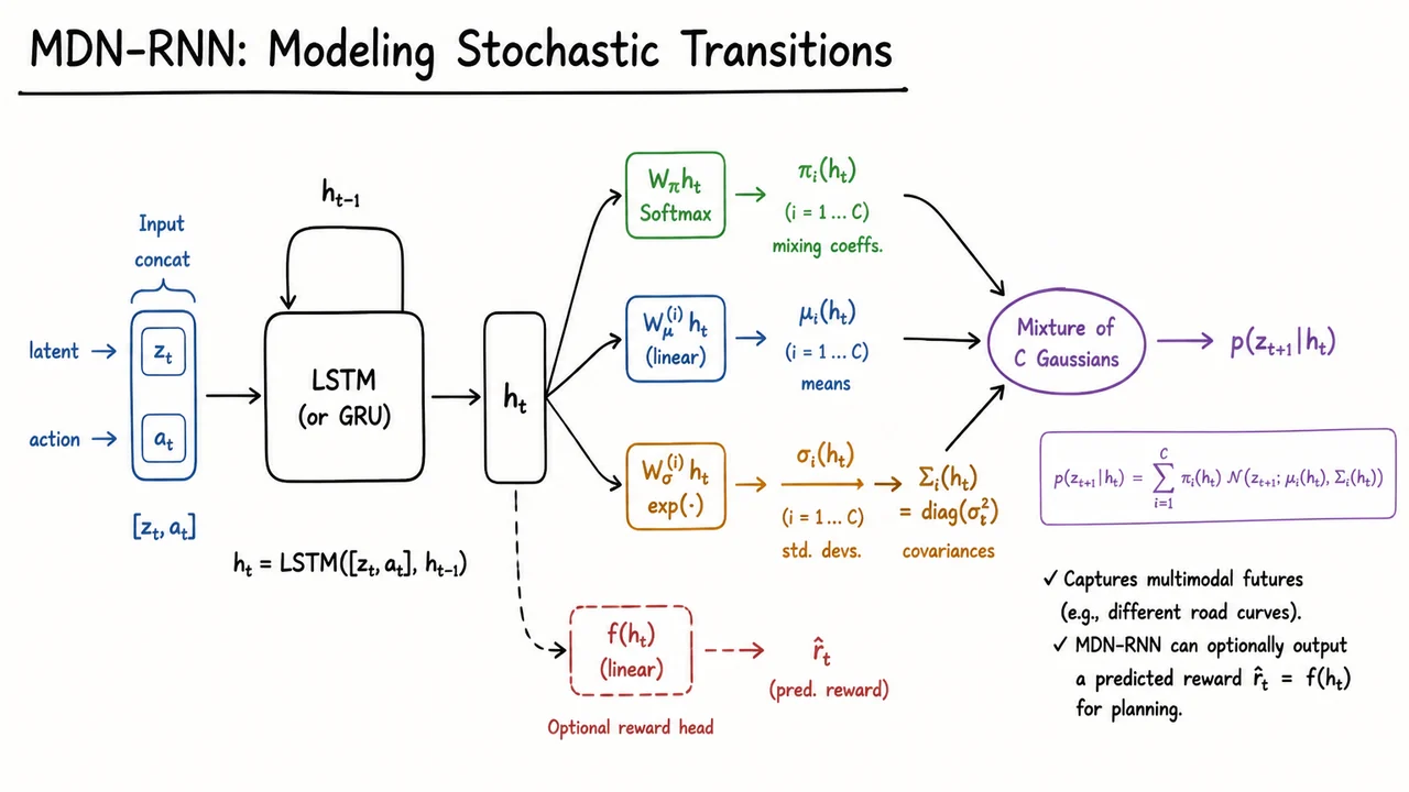
The backbone of this module is a recurrent network, typically an LSTM, which maintains an internal hidden state that summarizes the entire sequence of past latents and actions up to time . At each step the LSTM receives a concatenated vector along with its previous hidden state , and it produces an updated hidden state:
This formulation makes a rich, context-dependent representation. From we can parameterize a predictive distribution over the next latent . But rather than a single Gaussian, the MDN introduces a set of component distributions, each with its own mean and diagonal covariance, and a learned mixing weight that decides how likely each component is given the history.
The mathematics of this mixture is neat and expressive. The mixing coefficients are obtained by passing through a linear layer followed by a softmax, ensuring they sum to one:
Each component’s mean comes from its own linear transformation . To keep variances positive, we output log-standard-deviations and then exponentiate and square to form diagonal covariance matrices:
The full conditional density of given the history (summarized by ) is then
Here each term in the sum represents a plausible mode of the future—for example, one Gaussian component might concentrate around the latent code for a left-turn scenario, another around a right-turn. The mixing weights, being functions of the entire history, allow the model to increase the probability of the component that matches the actual observed outcome, adapting online as more evidence accumulates.
Why go to this trouble? A single diagonal Gaussian would force the model to cover all possible futures with one mean and one variance per latent dimension, which would either underestimate risk or average away important structure. The mixture model, by contrast, can split its probability mass. This is especially powerful in reinforcement learning because the agent can later sample diverse dreams from and plan accordingly. The MDN‑RNN also optionally outputs a predicted reward , making it a self-contained dynamics and reward predictor that can run entirely in latent space without ever rendering a pixel.
The visual below captures the entire flow in a compact schematic. On the left, the concatenated vector enters an LSTM block with a recurrent loop from the previous hidden state , producing . From there, three parallel heads branch horizontally: one applies a softmax to yield the mixing coefficients , another produces the component means via linear outputs, and the third exponentiates to give the standard deviations, from which diagonal covariances are assembled. All these parameters feed into a single mixture density node, which computes the rich multimodal distribution . An optional dashed path shows a reward prediction head, reminding us that the same compressed history can also estimate immediate rewards. The diagram’s hand-drawn aesthetic and distinct colors for each head make it immediately clear how the deterministic LSTM memory enables a stochastic, structured imagination of the future.
The previous section equipped the memory module with the expressive machinery of a mixture density network, enabling the RNN to emit a whole ensemble of Gaussian hypotheses for the next latent state. But predicting a rich distribution is only half the story; we must now define a training signal that will coax those hypotheses into alignment with the sequences of latent codes we actually observe. For a generative world model, the most principled signal is maximum likelihood: we want the MDN-RNN to assign high probability to the actual vectors that occur in recorded trajectories.
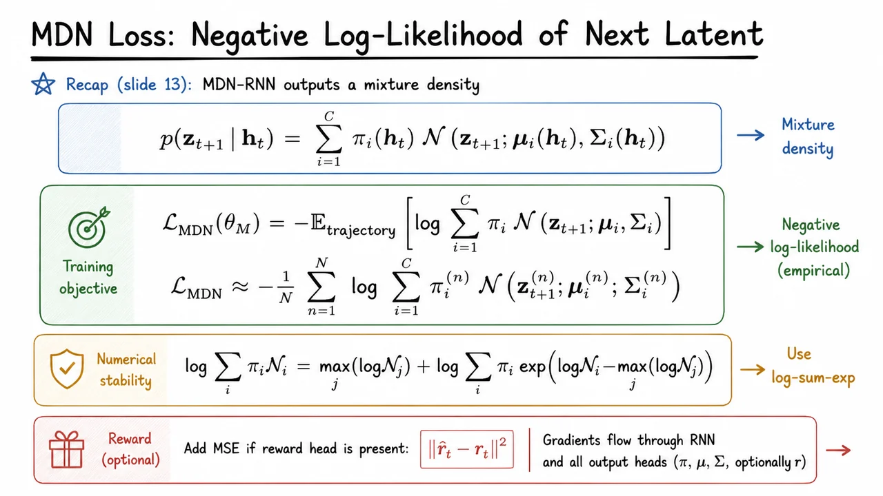
Concretely, at every time step the model receives the RNN’s hidden state , which summarizes the interaction history up to that moment, and as output it produces the mixing coefficients , the means , and the covariance matrices for . From these we construct the predicted distribution The log‑likelihood of a single transition is then the logarithm of this mixture evaluated at the observed next latent . To turn this into a loss for the RNN parameters , we simply minimize the negative log‑likelihood averaged over all transitions in our dataset:
In practice we approximate the expectation with an empirical average over a minibatch of sampled transitions, giving where the superscript indicates quantities computed for the ‑th sample. This objective directly encourages the mixture to place substantial probability mass where future latent vectors actually land, and through back‑propagation the RNN learns hidden representations that make the stochastic dynamics predictable.
Implementing this loss naïvely, however, is a recipe for numerical disaster. The mixture components can have very different scales: one Gaussian might assign an extremely low density to a given while another assigns a relatively high one. Summing these exponential quantities in original space often leads to underflow or overflow. The standard remedy is the log‑sum‑exp trick. First compute the log‑densities for each component, which avoids evaluating the exponential of a large quadratic form directly. Let . Then the log of the mixture can be stably computed as
Subtracting the maximum before exponentiation guarantees that the largest exponent is zero and all others are non‑positive, keeping the sum within a safe range. The final expression is then negated to obtain the loss contribution for that sample. Modern deep learning libraries offer functions like torch.logsumexp that implement this pattern, making the stable computation straightforward.
Optionally, the MDN-RNN can be augmented with a reward prediction head that outputs a scalar . In that case, a mean‑squared‑error term is added to the loss, with a suitable weighting, and gradients flow jointly through the RNN and all output heads (π, μ, Σ, and r). This multi‑task setup encourages the hidden state to capture information that is useful for both predicting future latents and anticipating imminent rewards, which directly benefits downstream policy learning.
The visual for this slide, titled “MDN Loss: Negative Log‑Likelihood of Next Latent”, condenses the entire training logic into a clean, hand‑drawn diagram. It begins with a brief recap of the mixture density, then stacks two highlighted boxes: the first shows the predictive distribution , and the second contains the negative log‑likelihood loss in large display math. A distinct call‑out for the numerical stability identity appears below, and a small note at the bottom reminds us of the optional reward MSE term. This layout mirrors the steps a practitioner follows: from model output to loss definition to stable implementation—a sequence that becomes second nature when training world models efficiently.
In the previous section we decomposed the negative log‑likelihood that a mixture density network (MDN) must minimize when predicting the next latent state . That loss, , captures how well the Gaussian mixture explains the true transition. But writing the loss is one thing; integrating it into a complete training loop for the recurrent memory module demands careful orchestration. The RNN that emits the mixture parameters must be taught to compress past observations and actions into a hidden state from which plausible futures can be drawn, all while respecting the temporal structure of the environment. That is where a structured training algorithm becomes essential.
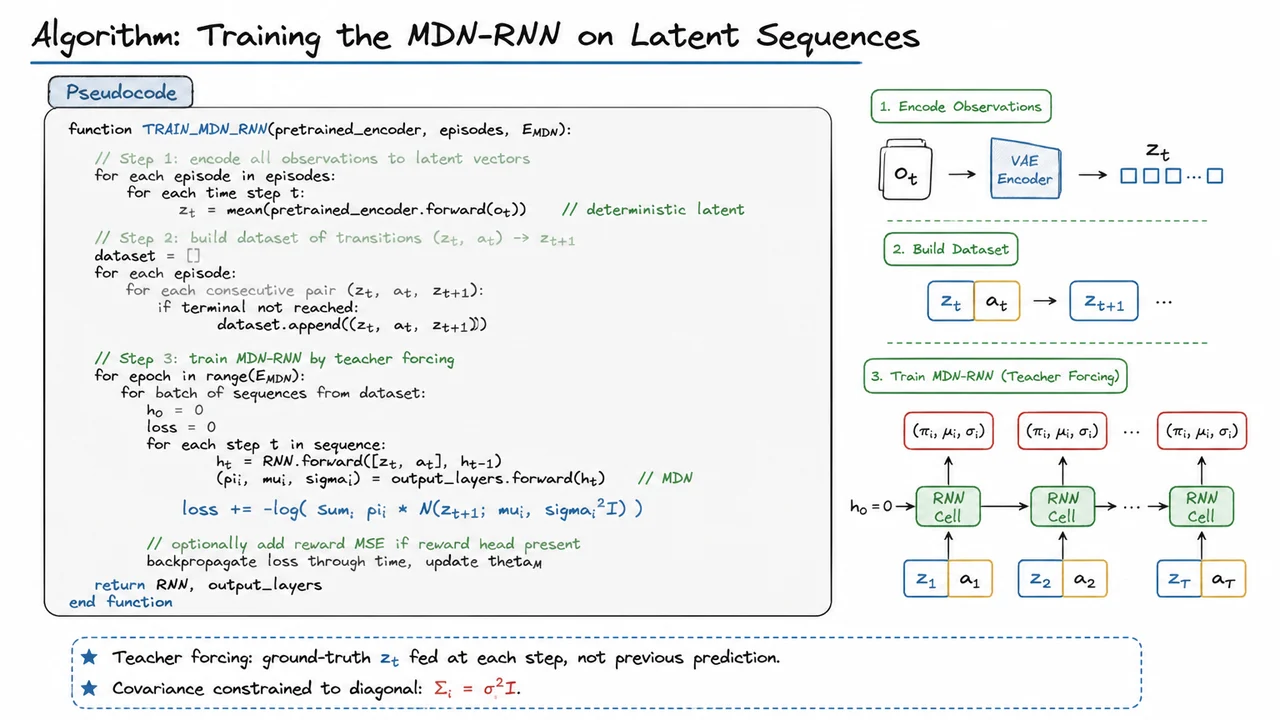
The training pipeline for the MDN‑RNN, often called the memory module of the World Models architecture, operates entirely in the compact latent space provided by a pretrained VAE. This decoupling is deliberate: the VAE is frozen, so the RNN never sees raw pixels and therefore can focus exclusively on learning the dynamics of the compressed representation. The procedure can be divided into three distinct phases: encoding all available experience into latent vectors, constructing a dataset of transition tuples, and finally training the recurrent model with teacher forcing. Each phase contains subtleties that affect stability and final prediction quality.
First, every observation collected across all training episodes is passed through the VAE’s encoder, but only its mean vector is retained as the deterministic latent . Sampling from the encoder’s distribution would inject noise into the training targets, making it harder for the RNN to learn a clean dynamics model. This choice reflects a pragmatic compromise: during imagination (rollouts from the RNN), we will later sample from the MDN’s own output distribution to reintroduce stochasticity, so we do not need the VAE’s variance at training time. The resulting latent sequences are aligned with the original action sequence and any terminal flags. If an episode ends at time , the transition from is simply discarded to avoid predicting across episode boundaries—a small but crucial housekeeping step that prevents the RNN from learning spurious continuations.
From these latent trajectories, a flat dataset of transitions is assembled: each entry is a tuple . Here is the action taken between the two latent states. The dataset may contain millions of such tuples, yet it represents a fixed memory of the agent’s past experience. This is the raw material that will be replayed epoch after epoch to train the dynamics model. Some implementations also store the immediate reward obtained alongside so that an auxiliary reward prediction head can be trained jointly, but the MDN‑RNN’s core task is to model state transitions.
The actual training loop then unrolls the RNN over contiguous sequences sampled from this dataset, using teacher forcing. That means at each time step the input to the RNN is the ground‑truth latent concatenated with the action , never a previously predicted . This stabilises learning because the model always conditions on correct context when computing the next output. Without teacher forcing, a single erroneous prediction early in the sequence would corrupt all later steps, creating a highly noisy learning signal. The hidden state is updated recurrently: , and from the output layers produce the mixture parameters . The MDN negative log‑likelihood of the true next state is then accumulated across the sequence, and gradients flow back through time to update all RNN and output parameters .
Notice the deliberate constraint placed on the Gaussian components: the covariance of each is diagonal, . This reduces the parameter count from to per mixture component and prevents the MDN from overfitting to the latent dimensions it deems easiest to predict, which would hurt generalisation when the RNN later runs in an autoregressive “dream” mode. It also keeps the loss computationally cheap, as the log‑likelihood of a diagonal Gaussian factorises into independent terms. The algorithm loops over the full dataset for epochs, by which time the model learns a rich stochastic transition function that can generate plausible future latents even when conditioned on its own earlier predictions, despite having been trained only with teacher forcing. This mild train‑test mismatch is empirically harmless because a well‑trained one‑step model tends to remain coherent over multiple autoregressive steps, especially in the low‑dimensional latent space of the VAE.
The accompanying diagram consolidates the entire procedure into a compact pseudocode block. It visually separates the three phases—encode, dataset, train—with indentation and high‑contrast comments, making the algorithm immediately scannable. The function signature TRAIN_MDN_RNN(pretrained_encoder, episodes, E_MDN) is emphasised, and inside the training loop the MDN loss equation appears prominently, connecting back to the earlier mathematical derivation. Below the code box, two terse bullet points remind the reader of the crucial design choices: teacher forcing and the diagonal covariance restriction. Used as a lecture companion, this pseudocode serves not as a line‑by‑line implementation manual but as a high‑level map of the three‑stage process, freeing the mind to reason about what happens when the trained RNN later begins to dream.
Once the MDN‑RNN has been trained to predict latent transitions from sequences of observations, a natural question arises: what does it actually think the future might look like? Moving beyond loss curves and latent-space statistics, we can directly visualize the model’s beliefs by sampling its predictive distribution and decoding the results back into image space. These inspections reveal whether the network successfully captures the irreducible uncertainty that a reinforcement learning agent will later need to plan around.
The heart of the memory module is a mixture density network that models a multimodal conditional likelihood over the next latent state . Concretely, given the current latent code , the action (for example, a steering angle in CarRacing), and the recurrent hidden state that summarises the past, the MDN‑RNN produces a distribution:
Here is the number of mixture components (commonly ), are the mixing coefficients, and each component is an isotropic Gaussian with mean and shared variance (scaled by the identity matrix ). This decomposition is not merely a convenient parameterisation; it reflects the model’s hypothesis that several distinctly different next states could be consistent with the same past experience and chosen action. A single Gaussian would force the prediction to collapse onto a single blurred average, erasing the very alternatives that a controller must learn to handle.
Why should such multimodality matter? Consider a driving scenario where the road forks, or where the car’s tyre grip varies randomly from moment to moment. A deterministic world model would secretly pick one outcome and commit the agent to an overconfident policy that breaks catastrophically when the real world diverges. In contrast, a multimodal distribution preserves multiple plausible futures, each of which can be explored during planning. The mixing coefficients represent the model’s estimated probability that the environment will in fact evolve into each mode, while the per‑component means capture the structural differences among the alternatives – for instance, a leftward curve versus a rightward curve when the road branches.
To turn these abstract latent predictions into something interpretable, we can sample the dream. For a single given context , we draw several independent realisations from the mixture and pass each through the VAE decoder to obtain imagined next‑frame observations. The decoder acts as a learned inverse of the compression process, mapping probabilistic latent points back to the high‑dimensional image space where we can visually assess the quality of the dream. Repeating this a handful of times exposes the range of behaviours the model considers probable under its own uncertainty.
What do these samples look like in practice? When we inspect a particular moment in a CarRacing episode, the actual current observation shows a road curving ahead. The driver takes an action, and the true next frame shows the car having moved slightly to follow a leftward bend. But the MDN‑RNN’s sampled futures from that same instant reveal a richer picture: some dreamt frames display the car entering a sharp left turn, others show a rightward curve, and a few stay nearly straight. This variation is not a sign of failure; it is exactly what we hoped the model would learn – the inherent stochasticity of the driving environment. Road forks, lateral drift, and momentary uncertainty about the car’s dynamics all naturally lead to a multimodal predictive distribution, and the model faithfully reproduces them without any explicit labels about road topology.
The visual that accompanies this explanation (a side‑by‑side comparison of the real observation, the real next frame, and five distinct dreamt samples) serves as an important validation checkpoint. It confirms that the MDN‑RNN has not just memorised a single high‑likelihood outcome but has genuinely internalised the multimodal uncertainty of the environment. The actual frames, typically outlined in a sober blue, anchor the comparison, while the dreamt frames – often shown with a contrasting border – make the spread of alternatives immediately tangible. Subtle cues such as small mean‑vector sketches or bar charts for the mixing weights can further clarify how the five Gaussian components distribute their probability mass across latent space.
Such visualisations are more than anecdotal illustrations; they build confidence that the controller, which will later be optimised entirely within the world model’s hallucinated rollouts, is exposed to a faithful and diverse distribution of future scenarios. If the model were to routinely miss plausible branches, the resulting policy would be brittle and unable to recover from surprises. The fact that a single input state can produce such qualitatively different dream outcomes underscores a key insight of the World Models approach: learning to dream means learning a generative model that acknowledges the world’s true stochasticity, and that is precisely what gives the agent the capacity to plan robustly. In the next stage, we will see how evolution strategies can train a compact policy directly inside this multimodal dream world, capitalising on the richness of the imagined futures.
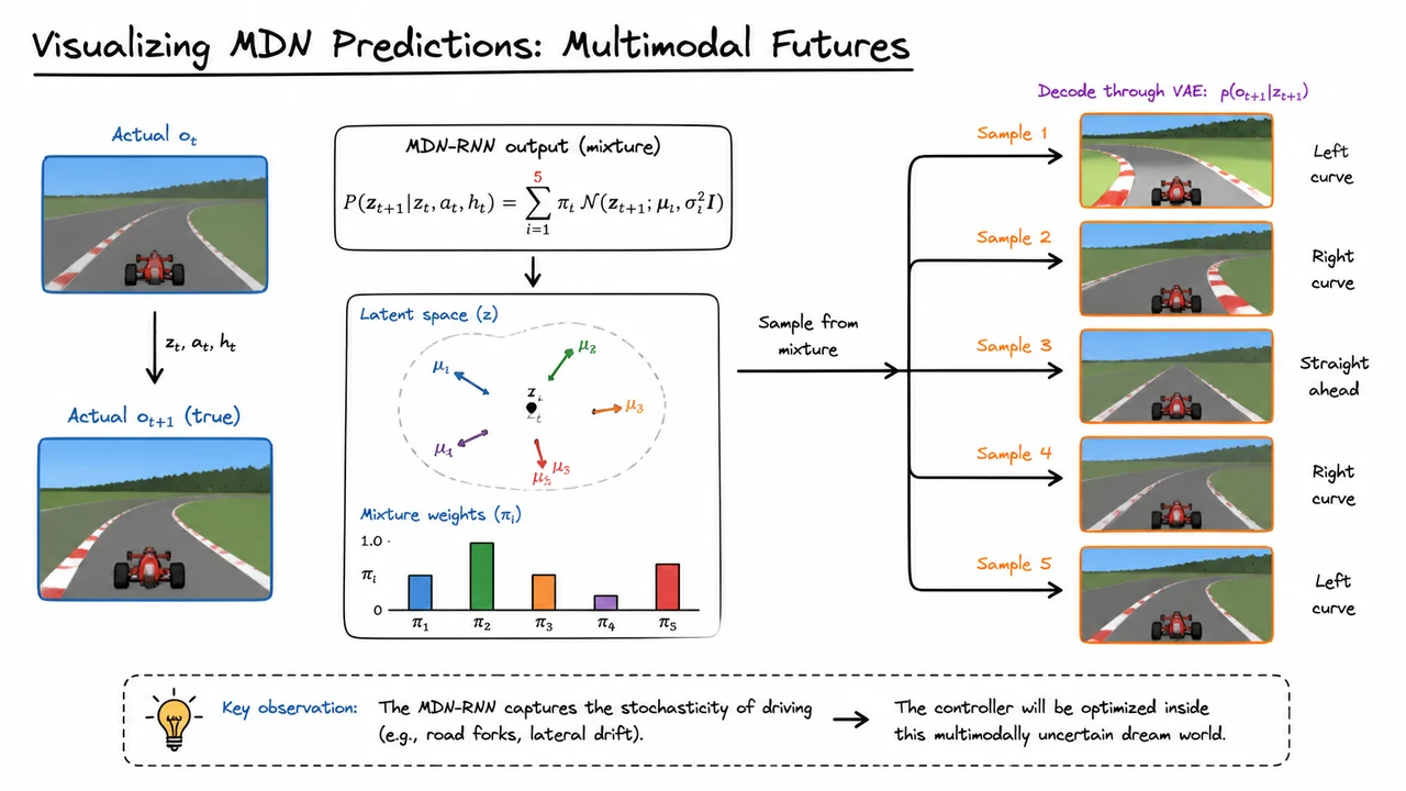
Having learned to compress observations into latent codes and to model the stochastic evolution of those codes with an MDN-RNN, we now possess a compact, generative world model that can be run forward in time without any interaction with the real environment. The dream engine is ready. What remains is to train an agent that can exploit this simulator to learn a policy. In the original World Models architecture, the controller—the piece that actually selects actions—is intentionally kept extremely simple: a single linear layer that maps the concatenation of the current latent state and the RNN’s hidden state to an action vector,
The controller has only a few hundred parameters, which at first glance seems too impoverished to solve a complex continuous-control task like CarRacing. Yet the central insight is that the world model already distills the environment’s dynamics and visual complexity; the controller merely has to learn a reactive mapping onto actions that maximises cumulative reward inside that model. This shifts the learning problem from high-dimensional pixel-based RL to low-dimensional latent-space optimisation, where a small linear policy can be surprisingly effective.
Training a controller inside a learned latent world model presents a different set of challenges from standard model-free RL. The dream environment is fully differentiable in principle (the VAE decoder is not used during dreaming, only the encoder and the MDN-RNN), so one might attempt to backpropagate a policy-gradient signal through time. In practice, however, the stochasticity introduced by the MDN’s sampling, the possibility of compounding errors over long imagined rollouts, and the desire to keep the controller small and easy to parallelise led the authors to adopt a black‑box optimisation technique: evolution strategies (ES). ES estimates the gradient of the expected cumulative reward with respect to the controller parameters by evaluating a population of perturbed parameter vectors, without ever requiring backpropagation through the RNN.
Concretely, we maintain a mean parameter vector (all weights and biases of the linear controller, flattened). In each generation we sample a batch of perturbation vectors . For each perturbed candidate we perform a full rollout inside the dream—starting from a realistic initial latent state, feeding the controller’s actions into the MDN-RNN, and accumulating the VAE-encoded rewards (or a reward predictor if available). The resulting cumulative reward serves as the fitness of that candidate. The gradient estimate is then the reward-weighted average of the perturbation directions:
We update the mean: (or use a more sophisticated optimiser like CMA-ES for better exploration). Because each dream rollout is cheap—no rendering, no real-time physics, just fast neural network evaluations—we can afford hundreds or thousands of parallel fitness evaluations, making ES highly competitive.
This approach elegantly circumvents the credit assignment problem that plagues reinforcement learning over long time horizons. The controller is never explicitly told which actions were good; it only sees a scalar score for the entire episode. ES converts the problem into a stochastic search over the parameter space, naturally handling the stochasticity of the MDN and the non-stationarity that arises from the evolving latent dynamics. Moreover, the ability to reset the dream to any starting state and to run many rollouts in parallel with different random seeds dilutes the impact of unlucky samples and allows the optimisation to rapidly converge to a policy that generalises to the real environment without any further fine‑tuning.
The visual below (Slide 17) distills this pipeline into a single glance. It depicts the flow from observation to latent code, the MDN‑RNN’s role as the stochastic transition model, and the compact linear controller that takes as input. Arrows wrap the ES loop around the dream rollouts, showing how a population of parameter perturbations is evaluated and how the fitness scores feed back to update the mean controller. This diagram is not merely an illustration; it is a structural summary of the World Models training phase, capturing the clean separation between representation learning (VAE), dynamics learning (MDN‑RNN), and behaviour learning (ES‑trained controller). Once you internalise that separation, the surprising efficiency of “learning to dream” becomes an intuitive design pattern rather than a trick.
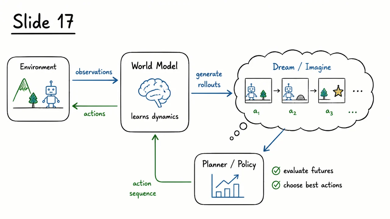
If you have spent any time training reinforcement learning agents on tasks that demand raw visual perception—say, steering a car in a top‑down racing game or navigating a procedurally generated maze—you will have felt the tension between sample efficiency and engineering convenience. Model‑free algorithms such as PPO, SAC, or DQN are remarkably general: they need almost no prior knowledge about the environment and can, in principle, discover sophisticated policies from pixels alone. Yet this generality exacts a steep price. To extract a meaningful signal from a high‑dimensional video stream, a model‑free agent often requires tens or even hundreds of millions of interactive steps, each one a full forward pass through a deep convolutional network and a careful credit‑assignment step. The bulk of these steps is spent rediscovering the same low‑level regularities—edges, textures, object boundaries—that could have been learned once and re‑used. This brute‑force approach makes model‑free RL exorbitantly expensive for real‑world or long‑horizon problems, and it gives the agent no explicit ability to plan, imagine, or anticipate the consequences of its actions.
World models offer a radically different path. Instead of learning a policy directly from observations, we first learn a compressed, predictive internal model of the environment itself, and then train a compact controller entirely inside that learned dream. The idea traces back to the predictive processing theories of the brain and echoes the classic “model‑based” thread in RL, but the key development of the World Models architecture is how to tightly co‑design a generative observation compressor, a stochastic forward model, and a minimalist policy so that the entire system can be trained with modest computation and a few thousand real environment frames. The pipeline decomposes into three modules: a Variational Autoencoder (VAE) that projects high‑dimensional frames into a dense latent code, a Mixture Density Network combined with a Recurrent Neural Network (MDN‑RNN) that learns the transition dynamics over those latent codes, and a compact controller that maps the RNN’s internal state to actions. Training the controller can even be done with gradient‑free evolution strategies (ES), completely sidestepping the need to backpropagate through the world model’s time‑unrolled predictions.
The VAE serves as the observation compressor. Given a sequence of raw images , we ask the encoder to produce a stochastic latent representation that is both low‑dimensional and sufficiently informative to reconstruct the frame accurately. The VAE objective balances a reconstruction loss (e.g., mean squared error over pixels) against a KL divergence term that pulls the approximate posterior toward a prior , typically a standard Gaussian. This forces the latent space to be smooth and compact, discarding pixel‑level noise while preserving the essential spatial and kinematic structure. In the CarRacing benchmark, for example, a 64‑dimensional latent vector can capture the position of the car, road curvature, and nearby obstacles, reducing a pixel frame by several orders of magnitude without losing the task‑relevant information.
Once we have a compact code, the MDN‑RNN learns to roll forward in that latent space. The RNN’s hidden state summarizes the history of past and actions , and its output is a Gaussian mixture model over the next latent vector . Why a mixture, and why not a deterministic point prediction? Real environments are stochastic—an agent’s actions may have slightly different outcomes due to physics noise, partial observability, or aliasing in the latent space. By predicting a full probability distribution, the MDN‑RNN captures this uncertainty explicitly; during dream rollouts, we can sample realistic future paths, and the controller becomes robust to the variability it will encounter later. The mixture parameters (means, variances, mixture weights) are trained to maximize the log‑likelihood of the observed under the RNN’s output distribution, typically with full gradient descent through the RNN unrolled for a few steps. Crucially, the VAE and the MDN‑RNN can be trained on a dataset of trajectories collected by a random or a naive policy—no high‑reward behavior is required at this stage. The world model is simply learning the “physics” of the environment.
With a dream generator in hand, the final step is to train a controller that produces actions given the RNN’s hidden state h_nor the latent vector—the network sees only the two‑dimensional latent code and the RNN’s memory, not the raw pixels. Because the world model is already doing the heavy lifting of compression and prediction, the controller can be remarkably small: often a single linear layer, or a tiny multi‑layer perceptron with a few dozen parameters. This minimal parameterization is not just an aesthetic choice; it makes the controller amenable to gradient‑free optimisation methods like **evolution strategies**, where we perturb the weights, evaluate the perturbed controllers over many imagined trajectories, and sum the rewards to estimate a natural gradient. Evolution strategies avoid the need for value functions, advantage estimates, or policy gradients computed over long, noisy horizons, and they naturally handle the non‑differentiability of the reward signal. Inside the dream, we can run thousands of parallel rollouts quickly, exploring a huge space of policies without ever querying the real environment. The synergy is what makes the approach so sample‑efficient. The VAE and MDN‑RNN may need only a few thousand real observations to become a passable simulator, and after that the controller’s entire search takes place “in the model’s head.” The CarRacing experiments in the original World Models paper (Ha & Schmidhuber, 2018) demonstrate a controller trained completely inside the dream achieving a score that surpasses a PPO baseline trained for many more environment steps. The dream’s fidelity does not need to be perfect; small modeling errors often act as a benign form of domain randomization, making the controller more robust when transferred back to the real environment. However, the dream also introduces a classic model‑bias risk: if the world model systematically misrepresents dangerous states or over‑simplifies dynamics, an evolution‑optimised policy can “overfit” to those inaccuracies and fail catastrophically upon deployment. Later work like Dreamer and MuZero refinement mitigate this by rolling out multiple imagined trajectories with repeated world‑model updates and by incorporating value learning, but the core insight—decoupling representation learning, dynamics learning, and policy search—remains. The visual below encapsulates the complete training pipeline in a single, glanceable diagram. It shows the three‑stage flow from raw pixel frames through the VAE bottleneck to a compact latent \(z_t; the MDN‑RNN that receives and an action , updates its hidden state , and emits a predictive distribution for ; and the compact controller that maps to the next action. Arrows indicate where evolutionary pressure is applied: the controller’s weights are optimised by ES using the cumulative reward from many dream rollouts, while the VAE and MDN‑RNN are pre‑trained on stored experience. The sketchy, hand‑drawn aesthetic reinforces the simplicity of the architecture—each module is a clean geometric block connected by a few carefully placed arrows. The diagram is not a dense schematic but an invitation to see the whole process as a composition of three clear, independently trainable functions, each solving a well‑defined subproblem. It turns what might feel like a sprawling system into a mental blueprint you can hold in your head.
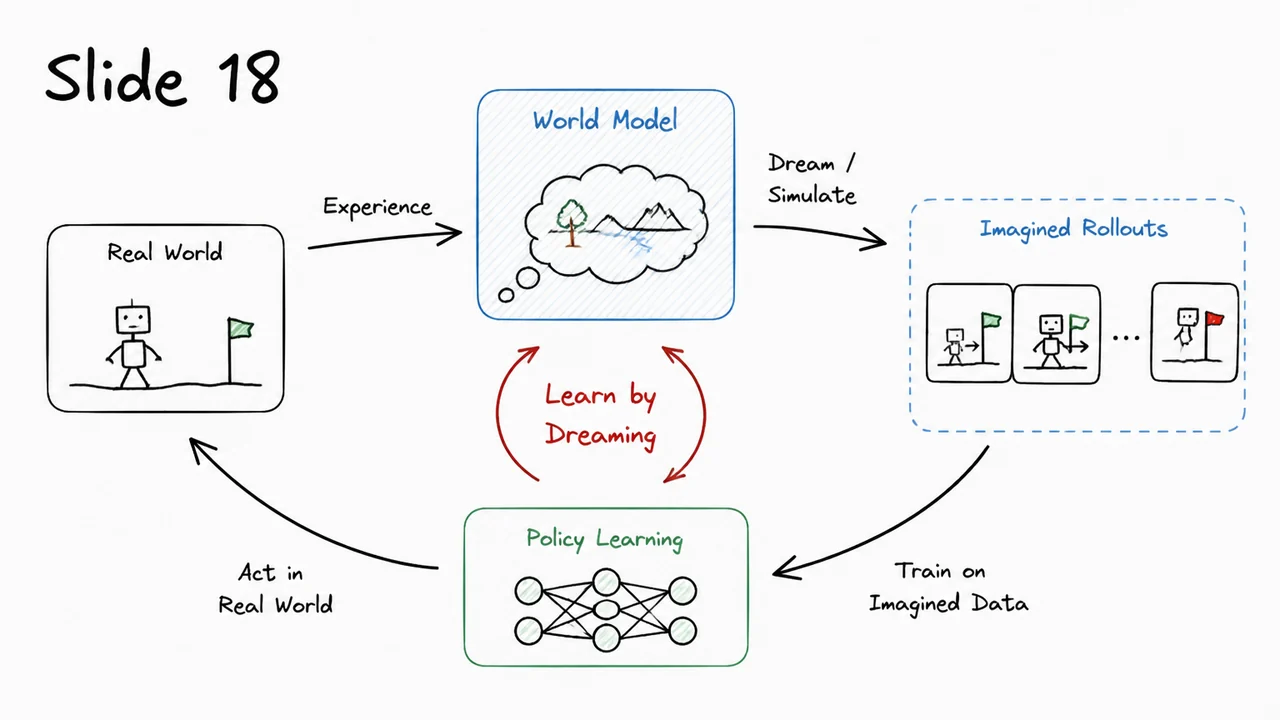
Model-free reinforcement learning has produced stunning results across games, robotics, and control tasks, but it carries a steep price: sample efficiency. A deep Q-network or policy gradient agent must interact with the environment millions of times, observing raw high-dimensional sensor readings, computing noisy reward signals, and slowly adjusting a massive neural network to map pixels to actions. Most of those interactions are spent re-learning basic physical facts about the world—how objects move, how collisions resolve, how the agent’s own actions change what it sees next. If the agent could instead build a compressed, predictive model of its environment, it could learn to act by “dreaming” inside that model rather than by repeatedly sampling the real world. This is the central insight behind World Models.
At a high level, a world model decomposes the RL problem into three trainable components, each addressing a distinct challenge. First, a Variational Autoencoder (VAE) compresses high-dimensional observations (e.g., 64×64 RGB frames) into a compact latent representation . Second, a recurrent dynamics model—often a Mixture Density Network combined with an RNN (MDN-RNN)—learns to predict the next latent state given the current latent and action . Finally, a lightweight controller maps a latent state (or a history of latents) directly to an action, and it is trained entirely inside the learned dream: the environment provided by the VAE and MDN-RNN together. Because the dream runs on compact tensors, training the controller becomes cheap enough that even black-box optimizers like Evolution Strategies (ES) become practical.
The VAE encodes the observation into a stochastic latent code by outputting the parameters of a Gaussian distribution, then sampling . The decoder reconstructs the observation, and the loss combines a pixel-wise reconstruction term with a KL divergence regularizer that keeps the latent distribution close to a prior (usually a standard Gaussian). This forces the latent space to be smooth, continuous, and information-dense—properties that the dynamics model will later exploit. Crucially, the VAE is trained once on a dataset of random or early-rollout observations and then frozen; the dream uses only the encoder (and optionally the decoder for visualization). The latent vectors are often 32- or 64-dimensional, a drastic reduction from the original pixel space.
With a fixed VAE, the MDN-RNN learns the environment’s transition dynamics in latent space. At each timestep, it receives the concatenation of and , and its RNN cell outputs the parameters of a Gaussian mixture model over the next latent vector . The mixture allows the model to capture multi-modal uncertainty—for instance, an agent approaching an intersection could turn left or right, leading to two distinct future scenes. The training objective is the negative log-likelihood of the observed latent sequence under the predicted mixture distribution. Because the latents are much lower-dimensional than images, the RNN can be small and its predictions are fast to compute, which is essential when the controller later asks for millions of simulated steps inside the dream.
The controller, typically a single-layer linear model or a tiny neural network, maps the current latent (and possibly the RNN’s hidden state) directly to an action. Why ES rather than backpropagation? The dream is a non-differentiable environment: the MDN-RNN outputs a probability distribution from which the next latent is sampled, and the VAE’s encoder may have stochastic elements. Computing meaningful gradients through many sampled timesteps is messy, while ES simply queries the controller’s parameters with small random perturbations, evaluates the total reward over a fixed horizon inside the dream, and adjusts the parameters in the direction of higher-performing perturbations. This derivative-free optimization sidesteps the credit-assignment complications and can be parallelized across many CPU cores, each running its own dream episode. The resulting controller is remarkably compact; in the original CarRacing experiments, a linear controller with fewer than 900 parameters sufficed to drive competitively.
Putting it all together, the training pipeline works in three phases:
This decoupling brings three enormous benefits. The world model learns once and can be reused for many tasks or reward functions. The agent can train for long horizons without ever touching a slow simulator or real robot. And because the controller sees only compressed latents, it is dramatically smaller and faster than end-to-end vision-based policies.
The visual below distills this architecture into a single flowing diagram. On the left, raw video frames enter the VAE’s encoder, which compresses them into compact latent vectors . Those latents, together with actions, feed into the MDN-RNN, whose recurrent core captures temporal dependencies and whose mixture density output models stochastic next states. The controller then lives entirely inside the dream loop: at each step it receives a latent state (and possibly the hidden state of the RNN) and emits an action that is passed back into the MDN-RNN, generating a new imagined latent. A reward predictor—often a simple linear head on the RNN’s hidden state—estimates the future reward, completing the closed dream environment. The entire cycle is repeated hundreds of steps, and evolution strategies evaluate many such dream rollouts to find a compact policy. The hand-drawn arrows and modular blocks emphasize that the three components are trained separately and then composed, turning the problem of learning from high-dimensional pixels into a problem of optimal control in a low-dimensional, learnable simulator.
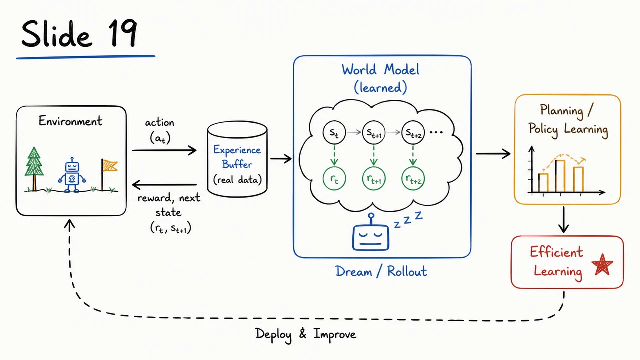
World Models take an unusual turn in their final component: they sidestep the standard reinforcement learning toolbox and instead train the agent’s policy with evolution strategies (ES). After compressing high-dimensional observations into a compact latent code and learning a predictive model that forecasts the next latent state and reward, we can now let the agent “live” entirely inside this learned dream. The controller—often just a small linear model or a shallow neural network—maps the current latent state and the RNN’s hidden state to an action . Training it means finding parameters that maximize the expected cumulative reward over dream rollouts. But why not simply apply a model-free RL algorithm, or backpropagate through the differentiable dynamics model? The answer reveals a key insight about the efficiency and robustness of the entire World Models pipeline.
Model-free deep RL algorithms, even when they manage to learn effective behaviors, tend to be horrifically sample-inefficient. They often require thousands or millions of environment interactions just to discover a reasonable policy, because they must simultaneously explore the environment, estimate value functions or policy gradients from sparse rewards, and deal with temporal credit assignment. In a learned world model, the agent can generate unlimited synthetic experience for free, but that doesn't automatically solve the credit assignment problem. Gradient-based approaches such as backpropagation through time (BPTT) can theoretically exploit the fact that the MDN-RNN is a differentiable model (or at least its mean predictions are), but BPTT over hundreds of dream steps can suffer from exploding or vanishing gradients, and the inherent randomness of the Gaussian mixture transitions makes exact gradients w.r.t. the reward sum noisy and often intractable. Moreover, the controller does not need to be remotely differentiable: evolution strategies treat the policy as a black box, requiring only the scalar fitness (total reward) as feedback. This decoupling grants enormous flexibility.
Evolution strategies operate on a remarkably simple principle: instead of computing the gradient of the objective analytically, they approximate it by sampling a small population of randomly perturbed parameter vectors and measuring how much the fitness (total reward) changes. Concretely, for a population of size , we sample perturbation vectors and form candidate parameters . Each candidate is run through a full dream rollout—starting from an initial latent state and hidden state , repeatedly querying the controller for actions and stepping the MDN-RNN forward—until a terminal condition is met, yielding a total reward . The ES gradient estimator is then a weighted sum:
This formula has an intuitive interpretation: perturbations that lead to above-average rewards get “pulled” in the positive direction, while those leading to poor rewards are effectively pushed away, because the sum weights each direction by the fitness achieved. Mathematically, this is an unbiased estimate of the gradient of a Gaussian-smoothed version of the objective, and it works even when the reward function is non-differentiable or noisy.
After computing the approximate gradient, the central parameter vector is updated with a learning rate :
This entire process is one generation. The algorithm then repeats for generations, each time sampling a fresh set of perturbations from the current . Notice that every candidate evaluation is independent and can be parallelized across multiple CPU cores or machines—dream rollouts are pure computation, requiring no interaction with the real environment. This parallelism is one of the main practical strengths of ES inside a learned world model: it can turn what would be a wall-clock nightmare for model-free RL into a few seconds of distributed dreaming.
There is a subtle but crucial detail about the dream’s stochasticity. The MDN-RNN, as a mixture density network, does not output a single deterministic next latent state; it predicts a Gaussian mixture distribution from which is sampled. This means two rollouts with identical parameters can different results, so the fitness is itself a random variable. The ES gradient estimator remains unbiased (with respect to the smoothed objective) as long as the perturbations are independent, but a larger population size may be needed to reduce variance when the dream is highly stochastic. In practice, World Models often use a population size of a few hundred, and a surprisingly compact controller—sometimes just a linear policy—can still learn remarkably sophisticated driving behaviors in environments like CarRacing.
The pseudocode in the accompanying visual captures this entire training loop in a compact block, making the abstract equations concrete. The outer loop iterates over generations, the inner loop evaluates the population, and the final lines perform the gradient estimate and parameter update. The highlighted equations for and the update step are displayed as central anchored formulas, while the note below the box clarifies that MDN_RNN_step draws from the predicted mixture and returns the immediate reward. The hand-drawn aesthetic, with line numbers and subtle amber highlights, draws the eye precisely to the gradient computation—the core innovation that frees the controller from the shackles of backpropagation and model-free credit assignment.
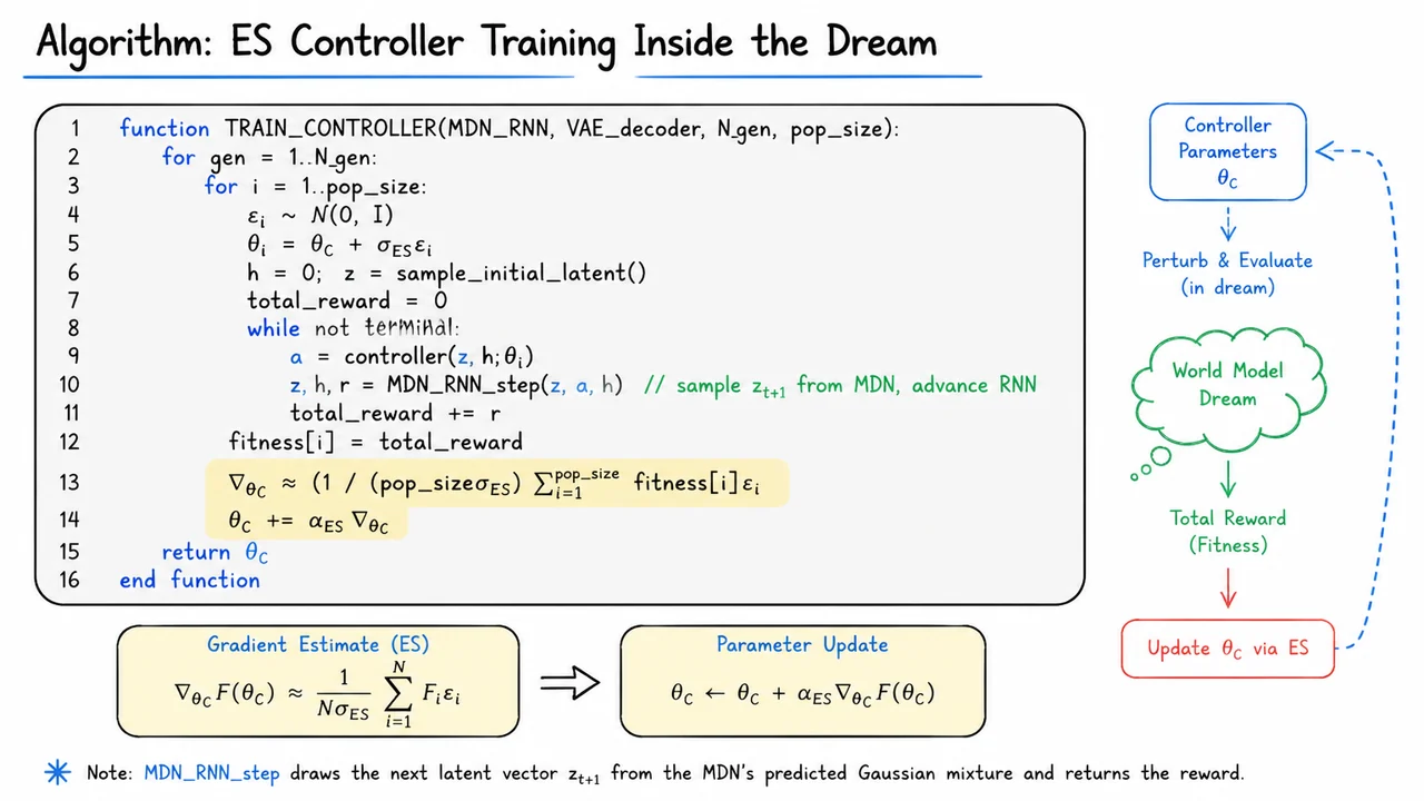
Throughout the previous section, we zoomed in on the mechanics of training a compact linear controller entirely inside the “dream” generated by the world model. Evolution strategies proved to be a surprisingly effective—and embarrassingly parallel—way to discover a policy that maximizes the imagined cumulative reward, without ever touching real environment roll‑offs for policy updates. But this training loop is only the final stage of a much larger idea. To appreciate why the world models approach marked a turning point in model‑based reinforcement learning, we need to pull back and examine the complete pipeline: a tripartite agent whose visual cortex, memory, and decision‑making module are each trained with separate, focused objectives.
The heart of the architecture is a variational autoencoder (VAE) that compresses high‑dimensional RGB frames into a compact latent code . The VAE is trained purely on static observations, without any notion of time or reward. Its loss combines a pixel‑wise reconstruction term with a KL regulariser that keeps the latent distribution close to a standard Gaussian. This gives us two critical properties: the latent space is smooth and continuous, and we can sample from it to later generate imagined frames. Once the VAE is fixed, we never feed raw pixels to the temporal modules; instead, every future frame is represented by its latent vector.
Next comes the mixture‑density recurrent neural network (MDN‑RNN), which learns to model the environment’s dynamics over time in this compressed space. Rather than predicting a single deterministic next state, the MDN‑RNN outputs the parameters of a Gaussian mixture model for the next latent and for the reward . Training minimizes the negative log‑likelihood of the actual next latent and reward under the predicted mixture. During the dreaming phase, the RNN’s deterministic hidden state is updated using the sampled and action , and then the next latent is drawn from the mixture. This stochastic imagination is essential for capturing the unpredictable aspects of a complex environment, such as the random track generation in CarRacing.
The third component, the controller, is a small neural network (or even a linear model) that maps the concatenated representation to an action . Critically, the controller is trained entirely inside the imagined roll‑outs produced by the MDN‑RNN. By fixing the VAE and the world model, the agent can simulate thousands of parallel dreams, evaluating each candidate policy’s average dream reward. Evolution strategies (ES) perturb the controller’s parameters, run dream episodes, and move the mean towards higher‑reward perturbations—all without back‑propagating through time or interacting with the real environment. This separation of representation learning, dynamics learning, and policy improvement yields a remarkably sample‑efficient system: the VAE and MDN‑RNN are trained once on a static dataset of agent experience, and the controller can be refined extensively inside the dream with zero additional environment steps.
Empirical results on the CarRacing‑v0 benchmark vividly demonstrated the power of this separation. The world‑model agent achieved a super‑human score while using only a fraction of the environment interactions required by state‑of‑the‑art model‑free methods. However, the experiments also exposed several failure modes that motivated later work. The VAE, while effective at compressing frames, sometimes blurs out crucial details (like a sharp turn or a close obstacle) because it optimizes pixel‑wise likelihood, which is agnostic to the downstream control task. The MDN‑RNN’s predictions drift over long horizons, and errors compound, causing the controller to exploit dream inconsistencies that do not exist in reality. Moreover, training the three modules in strict sequence—first VAE, then MDN‑RNN, then controller—prevents any mutual adaptation and can lead to sub‑optimal latent representations for the specific goal at hand.
These shortcomings spurred a wave of extensions that integrate representation, dynamics, and policy learning more tightly. Dreamer (Hafner et al., 2019) learns a latent dynamics model that is trained jointly with an actor‑critic agent in the latent imagination, using pixel reconstruction only as an auxiliary signal and back‑propagating value gradients through imagined trajectories. This allows the world model to adapt its representations to the needs of the policy. MuZero takes a different tack: it completely discards explicit reconstruction and instead learns a hidden‑state representation and a dynamics function that are trained end‑to‑end solely from reward, value, and policy predictions. MuZero’s use of Monte‑Carlo tree search inside its learned model achieves superhuman performance in Atari, Go, and chess, demonstrating that a world model can be entirely task‑driven.
The visual below synthesizes the full World Models pipeline and its most influential descendants. At the center, you see the original three‑module flow: high‑dimensional observations are compressed by the VAE into , then fed with actions into the MDN‑RNN, which predicts future latents and rewards while maintaining a hidden state . The compact controller uses and to choose actions, and it is optimized inside the dream via ES. Surrounding this core are branches that illustrate how Dreamer and MuZero alter the recipe—Dreamer jointly optimizes the latent dynamics and the policy using value gradients, while MuZero replaces pixel reconstruction with reward/value/policy predictions and adds tree search. The diagram serves as a quick mental map of the conceptual leap from dreaming with a frozen model to fully integrated model‑based reasoning, reminding us that the original World Models blueprint was not an end point but the ignition of a rich research programme.
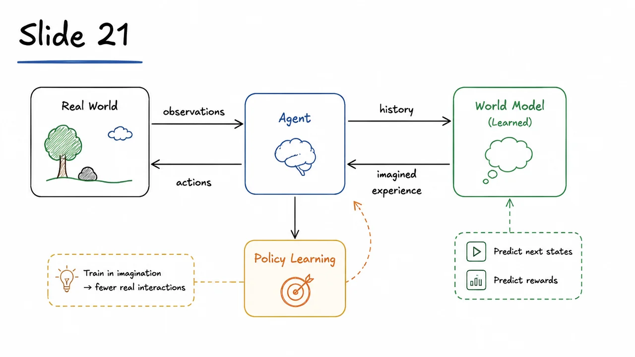
The most striking limitation of modern deep reinforcement learning isn’t a lack of clever algorithms—it’s the staggering number of environment interactions needed to master even simple tasks. A model‑free policy gradient method can require millions of frames to reach human‑level performance on an Atari game or a driving simulator. Each frame corresponds to a real step in an environment, and in robotics or other physical domains that cost is measured in time, money, and safety. This inefficiency betrays a deeper problem: the agent is learning only from a reward signal that arrives after a long, noisy sequence of actions, with no internal model of how the world responds to its choices. Humans, by contrast, build rich mental models that let us imagine the consequences of our actions without ever leaving our chair.
World models reframe the RL problem by giving the agent the ability to dream—to simulate future trajectories inside its own compressed representation of the environment. Instead of demanding millions of expensive real‑world samples, we first teach the agent a compact, predictive picture of its observations and dynamics. Then we train a compact policy entirely within that internal dream, occasionally checking whether the policy still works when deployed to the real world. The philosophy is disarmingly simple: if the model is good enough, dreaming is almost as good as doing. This shift can reduce the required environment interactions by over an order of magnitude while still producing capable behavior.
The classic world‑models architecture, proposed by Ha & Schmidhuber (2018), has three components that are trained sequentially. First, a variational autoencoder (VAE) compresses high‑dimensional observations—such as pixel frames from a car‑racing game—into a low‑dimensional latent vector that retains the essential perceptual information. The VAE is trained on random rollouts to maximize the evidence lower bound (ELBO), balancing reconstruction fidelity with a KL‑divergence regularizer that keeps the latent distribution close to a unit Gaussian. By doing this, the agent learns a disentangled, compact code that discards irrelevant pixel‑level noise while preserving the position of the car, road boundaries, and other salient features.
Second, a mixture‑density recurrent network (MDN‑RNN) learns to model the temporal evolution of these latent states. Given the current latent vector and the action selected by the agent, the RNN produces the parameters of a Gaussian mixture model that captures the distribution over the next latent state . Crucially, this allows the model to be stochastic: it can represent multi‑modal futures (e.g., the car could skid left or right on a slippery turn) and propagate uncertainty across time. The MDN‑RNN is trained by maximizing the log‑likelihood of observed latent sequences, so it learns a predictive world dynamics simulator that runs entirely in latent space.
The third component is a controller—often a small, linear or one‑layer neural network—that maps the latent state and the RNN’s hidden state to an action . Because the world model already handles perception and planning, the controller can be extremely lightweight. Instead of backpropagating through the dynamics model (which would be expensive and prone to compounding errors), the controller’s weights are optimised using evolution strategies (ES). ES perturbs the weight vector, runs the agent inside the dream environment, and uses the total reward of a simulation as a fitness score to update the population mean. This black‑box approach neatly sidesteps the need to compute gradients through the RNN and VAE, and it can efficiently explore policy space using parallel rollouts in the cheap dream world.
A natural concern is whether a policy trained purely in a learned dream will ever work in reality. The CarRacing benchmark provides an elegant testbed. After training the VAE and MDN‑RNN on a dataset of random driving, the controller is evolved inside the dream—never seeing a single real game frame during training. When the evolved policy is finally deployed to the actual game, it drives competently along the track, sometimes even discovering smooth drifting behaviors that were never explicitly taught. This dream‑to‑reality transfer demonstrates that a sufficiently accurate latent dynamics model can substitute for the real environment during the intensive phase of policy search.
Of course, the approach is not magical; it comes with a set of failure modes and spins off several powerful extensions. If the VAE’s latent space discards task‑relevant details, the dream becomes impoverished and the policy overfits to a world that doesn’t match reality. The MDN‑RNN can suffer from compounding prediction errors over long rollouts, causing the dreamed trajectories to diverge into unrealistic states. Subsequent work like Dreamer and MuZero addresses these issues by integrating planning directly into latent space, learning a world model and a policy end‑to‑end with imagined rollouts and value estimation, and even by using the model to plan ahead inside a Monte Carlo tree search. These advances blur the line between model‑based and model‑free RL and demonstrate that dreaming can be made robust enough for complex, high‑dimensional tasks.
The visual below distills the entire architecture into a clean, three‑stage pipeline. On the left, raw pixel frames are encoded by the VAE into a compact latent vector . The central module, the MDN‑RNN, takes this latent state together with the previous action and outputs a distribution over the next latent state, effectively stepping the dream forward in time. Finally, the small controller, whose weights are evolved rather than backpropagated, receives the current latent state and hidden state and emits the next action. This diagram doesn’t just summarise the flow of data; it makes the separation of concerns immediately obvious: perception, dynamics, and action are cleanly partitioned, which is precisely what enables the sample efficiency and modularity that make world models so compelling.
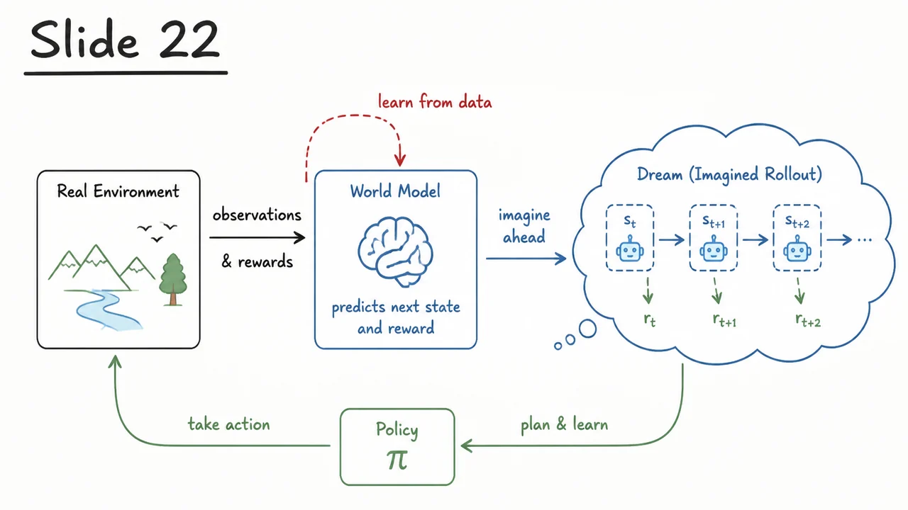
If a reinforcement learning agent can learn to act by dreaming inside a world model trained solely on random exploratory data, then an enormous practical bottleneck dissolves: the need for millions of task-specific interactions with a real environment. The World Models architecture tests this hypothesis in a visually rich continuous control domain, CarRacing‑v0, where the agent must steer a car around a track using only pixel observations. The results are striking: a compact policy trained entirely in hallucination transfers zero‑shot to the real environment and outperforms a heavily optimized model‑free baseline while consuming two orders of magnitude fewer real steps. This section unpacks that experiment and its dream‑to‑reality transfer.
The CarRacing environment demands from the agent raw 96×96 pixel frames and outputs continuous steering, acceleration, and brake commands. A standard model‑free approach such as an actor‑critic agent (A3C) requires over 100 million real steps to reach a score of roughly 600, slowly improving from scratch through trial and error. World Models takes a radically different path: it first learns a compact, latent generative model of the visual dynamics using completely random rollouts—no reward signal, no directed exploration—and then trains a controller entirely inside the resulting dream. The three‑stage pipeline (VAE, MDN‑RNN, controller) that was described in the previous section is exactly what makes this possible.
Only 10 000 random rollouts are collected, amounting to about 10 million real environment steps. The variational autoencoder (VAE) compresses each observation into a low‑dimensional latent vector , and the mixture‑density recurrent network (MDN‑RNN) learns to predict the next latent state together with a distribution over future rewards, all conditioned on the current latent state and its own hidden state . After this phase, the real environment is set aside. The world model now acts as a fully self‑contained simulator: given an initial latent encoding and an action, the MDN‑RNN advances its hidden state and generates the next perceived latent state, effectively dreaming an infinite stream of possible futures.
Inside this dream, a simple linear controller is optimized using evolution strategies (ES). The controller sees only the concatenated latent and recurrent state, producing an action, and ES evaluates entire imagined episodes—earning rewards entirely from the dreamt reward predictions—to iteratively update the weight matrix and bias . Because the latent space is small and the policy is linear, the search is fast and sample‑efficient without any backpropagation through time. No real environment feedback is used; the entire learning of the control policy happens exclusively within the hallucinated rollouts.
Once the dream‑trained policy converges, it is deployed in the real CarRacing environment in a zero‑shot fashion. Real pixel frames are encoded via the VAE encoder , the MDN‑RNN maintains its hidden state as it runs forward, and the controller maps the combined directly to actions. There is no fine‑tuning, no adaptation—the agent simply acts using the policy it acquired while dreaming. Remarkably, this transfer works reliably, achieving a mean score of 906 ± 21 over 100 trials, while the A3C baseline plateaus around 600 after more than ten times the real‑world experience.
| Method | Real Environment Steps | Mean Score (100 trials) |
|---|---|---|
| World Models (V+M+C) | 10 M (random data) | 906 ± 21 |
| A3C (continuous) | >100 M | ≈ 600 |
This table distills the core argument: sample efficiency and final performance need not be in tension when a world model can convert random experience into a rich, reusable forward simulator. The controller is never exposed to the real task during training, yet it surpasses an agent that spent over 100 million steps specifically practicing the driving task. The reason is the dream’s fidelity—even though the latent predictions are imperfect, they preserve enough structure about track boundaries, speed, and steering dynamics that an evolution strategy can discover robust behaviors.
The visual below encapsulates these findings in a compact comparison. A bar chart places the two methods side by side, with the model‑free A3C bar reaching roughly 600 and annotated with “>100 M real steps,” while the World Models bar climbs to 906 with a narrow uncertainty whisker and the label “10 M real steps (random data).” This immediate contrast reinforces the 10× reduction in real experience and the substantial performance margin. Just as telling is the small inset showing a sequence of four decoded latent frames—hallucinated grayscale car images—generated entirely by the dreaming MDN‑RNN. The world model’s predictions, though blurred and slightly distorted, clearly depict the road and car position, giving a qualitative sense of the dream fidelity that enables the controller to learn. Together, the chart and the dream frames make it plain: dreaming is not merely a metaphor; it is a viable, highly sample‑efficient training regime for continuous control from pixels.
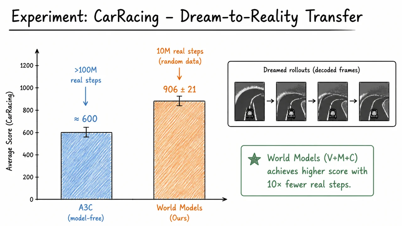
While the CarRacing experiments demonstrated a full dream-to-reality transfer with a compact controller, the VizDoom scenario sharpens the story in two directions: it shows just how little real data a world model can need, and it exposes exactly where the compressed visual pipeline breaks. In the basic VizDoom take‑cover shooting task, the agent sees first‑person 64×64×3 RGB frames and receives a reward for each enemy it kills. The world model must learn to reconstruct these frames, to predict how the latent state evolves under actions, and to support a policy that aims center‑of‑screen and fires. What makes the result striking is that the entire real‑world interaction budget is roughly 1 000 steps – a tiny fraction of the millions of frames a model‑free baseline like A3C typically consumes.
The world model follows the same three‑component recipe as before, scaled to the new observation space. A convolutional VAE compresses each 64×64×3 frame into a compact latent vector . The encoder is trained to minimise the usual reconstruction loss plus a KL‑divergence penalty, forcing to capture the essential structure of the scene while smoothing out irrelevant detail. After the VAE is trained on frames collected from random rollouts (those same ∼1 000 steps), an MDN‑RNN is taught to model the stochastic dynamics by predicting the parameters of a Gaussian mixture distribution over the next latent state. Here denotes the RNN’s hidden state, which provides a memory of previous observations and actions. The key is that the MDN‑RNN never sees the raw pixels; it only ever encounters the compressed latents and the discrete actions . This decoupling lets the dynamics model be both compact and fast when running forward in the agent’s imagination.
Finally, a linear controller maps the concatenation of the current latent and hidden state directly to motor commands (turn left/right, shoot, etc.). Because the controller contains only a few hundred parameters, it can be efficiently optimised with evolution strategies (ES) entirely inside the dream. At each generation, the algorithm samples perturbation vectors and evaluates the total reward obtained by rolling out the perturbed policy in the imagined environment. The parameter update follows the standard ES gradient estimator:
Because every rollout is a fast, batched forward pass through the RNN and the linear policy, the dream can run at hundreds of frames per second, enabling ES to evaluate thousands of candidate policies per second. This raw throughput translates a handful of real interactions into an optimisation loop that feels almost instantaneous compared with online RL.
The empirical payoff is remarkable. With only the initial 1 000 real steps used to train the VAE and the MDN‑RNN, the linear controller evolves inside the dream to achieve average scores that are competitive with an A3C agent trained on millions of real environment steps. In other words, the world model extracts so much structure from the limited real frames that dreaming alone suffices to learn a competent shooting behaviour. The speed advantage is not just an implementation detail; it is what makes the ES loop practical, since a single real step would otherwise be far too expensive to evaluate thousands of perturbations. This efficiency gain is one of the central promises of world‑model‑based RL: separate the slow, data‑intensive learning of perception and dynamics from the rapid, compute‑intensive policy search.
However, the VizDoom experiment also exposes a fragility that is easy to overlook when scores are reported in a static environment. The VAE encodes a specific visual distribution seen during training. If the environment changes – for example, if the wall textures are altered after deployment – the encoder produces latent vectors that do not faithfully represent the true state. Because the MDN‑RNN was never exposed to these novel latents, its predictions drift, and the policy receives misleading inputs. The result is a catastrophic drop in performance, often total inaction or random wandering. The visual compression that made dreaming cheap suddenly becomes a liability when the sensory statistics are no longer stationary.
The accompanying visual condenses these findings into two panels that mirror the contrast between remarkable efficiency and distributional brittleness. On the left, a log‑scale learning curve plots average episode score against the number of real environment steps. A solid “World Models (dream only)” curve rises sharply after only a few hundred real frames and soon rivals a dashed “A3C (real steps)” line that requires millions of interactions to reach similar performance. A vertical dashed line at 1 000 real steps annotates the tiny data budget used by the world model. On the right, side‑by‑side images show an original VizDoom frame with default wall textures and a modified frame where the walls have a strikingly different appearance. Below each frame, the VAE’s reconstruction reveals the damage: the reconstruction of the original texture is clean, while the altered texture collapses into a blurry, distorted mess – the visual manifestation of a collapsed policy. The figure makes tangible the lesson that compressed world models can dream efficiently, but they dream only of the world they have seen.
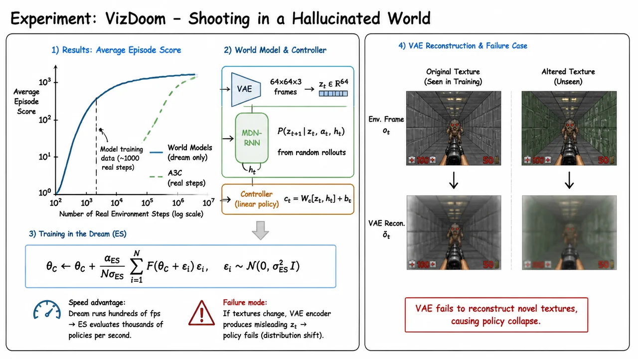
The VizDoom experiment we just examined is a compelling proof of concept: an agent trained entirely inside its own generative model can perform meaningful tasks when that model is reconnected to a real environment. That experiment hinted at a more general recipe, one that the World Models paper develops into a surprisingly simple yet powerful pipeline for solving high-dimensional reinforcement learning tasks, most notably the CarRacing environment. Understanding this pipeline from end to end—how a variational autoencoder, a recurrent stochastic dynamics model, and a linear controller fit together—reveals both the elegance of the approach and the failure modes that later work like Dreamer and MuZero would systematically address.
The starting point is the observation that model‑free RL spends an enormous number of environment interactions just to form a compact, reusable representation of the visual world. A human driver does not need to re‑learn the physics of pixel‑level motion every time they approach a turn; they have an internal model of how the scene will evolve. The World Models pipeline externalises this intuition in three stages. First, a Variational Autoencoder (VAE) compresses each high‑dimensional observation frame into a low‑dimensional latent vector . The VAE is trained by maximising the evidence lower bound: where a small can be used to balance reconstruction fidelity against latent regularity. This yields an encoder that maps raw pixels to a compressed code and a decoder that can rebuild the image when needed—though, crucially, the decoder is only used for inspection; the agent itself never sees the reconstructions during policy learning.
Next, a Mixture Density Network combined with a recurrent neural network (MDN‑RNN) models the temporal evolution of these latent states. At each time step, the MDN‑RNN takes the current latent and its hidden state and outputs the parameters of a Gaussian mixture model over the next latent state and an estimate of the reward —and optionally whether the episode terminates. Training minimises the negative log‑likelihood of the observed sequences of latents and rewards: Because the RNN maintains a deterministic hidden state that summarises the past, the mixture over the next latent state captures the residual stochasticity of the environment—a reflection of things the agent cannot perfectly predict, such as the behaviour of other cars or the precise texture of the roadside. Once trained, this model can be rolled forward in a closed loop, generating an endless stream of hallucinated latent trajectories and rewards, a process the authors call dreaming.
The final piece is the controller, which maps the latent and the MDN‑RNN’s hidden state directly to an action . The original World Models paper uses an elementary linear model: The simplicity is deliberate: it forces the world model to organise the latent space and recurrent dynamics in a way that makes the control problem almost linearly separable. To train this controller without requiring differentiability all the way back through the RNN and VAE—and to avoid the fragile credit assignment of back‑prop through time—the paper employs Evolution Strategies (ES), specifically CMA‑ES. A population of controller parameter vectors is sampled, each is evaluated by running many episodes inside the dream environment, and the cumulative reward guides the search. This decouples the world‑model training (supervised, stable) from the policy optimisation (gradient‑free, robust to non‑smooth reward landscapes), and the entire controller training can be done purely in hallucination, needing zero additional real‑environment steps.
The CarRacing benchmark became the canonical test of this procedure. After collecting around 10,000 random rollouts, the VAE and MDN‑RNN were trained offline. Then ES optimised the linear controller for hundreds of generations, each evaluating an agent entirely on dreamed latent trajectories. The result was remarkable: a compact linear policy that steered smoothly, stayed on the road, and even learned to accelerate out of turns, achieving a score competitive with model‑free algorithms that required orders of magnitude more real interactions. However, several failure modes crept in. The VAE’s reconstructions were often blurry, sometimes smearing out fine details like distant obstacles or the exact shape of the kerb; the RNN’s predictions accumulated error over long rollouts, causing the dream to drift away from the real environment’s dynamics; and the linear controller, while surprisingly capable, sometimes failed to represent nuanced behaviours needed for complex corners or recovery from mistakes. When the dream was poor, the real‑world transfer suffered.
These limitations spurred a generation of successors. Dreamer (Hafner et al., 2020) replaces the VAE and MDN‑RNN with a Recurrent State‑Space Model (RSSM) that learns a factored latent representation—combining deterministic and stochastic components—purely from sequences, and then trains an actor‑critic agent by back‑propagating value gradients through the imagined latent trajectories. It never reconstructs images, instead using a contrastive or predictive loss in latent space, which yields sharper world models and more effective behaviour learning. MuZero (Schrittwieser et al., 2020) pushes the idea further: it learns a dynamics model that predicts future values, policies, and rewards directly, without any reconstruction objective or latent uncertainty model. Combined with Monte Carlo tree search, MuZero masters Atari, Go, chess, and shogi from the same architecture, showing that dreaming can be made even more abstract while achieving superhuman performance.
The visual summary below distills the original World Models training pipeline into a single diagrammatic glance. The VAE encoder compresses real frames into latent vectors, the MDN‑RNN learns to roll forward these latents while predicting rewards, and the compact linear controller, trained purely in the dream via evolution strategies, maps the joint latent‑and‑hidden state directly to actions. Arrows capture the flow of information during training and deployment, and the separation into a world‑model phase (supervised) and a dream‑policy phase (ES) is made explicit. This skeleton reveals the core insight—that a well‑structured world model can abstract perception and dynamics so cleanly that even the simplest policy optimisation becomes powerful—while also hinting at the cracks that Dreamer and MuZero would later seal.
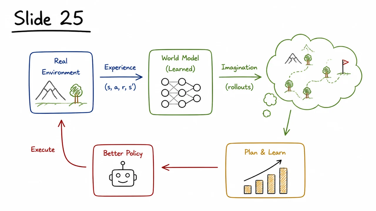
Model-free reinforcement learning algorithms can master complex tasks, but they often demand millions of interactions with the environment – a luxury that physical systems, high-fidelity simulators, or even impatient researchers rarely afford. Each real-world step requires collecting an observation, selecting an action, and waiting for the next state and reward. The bulk of this computational budget is spent on learning a value function or a policy that directly maps raw, high-dimensional observations to actions without explicitly modeling the environment’s mechanics. If we could instead compress the important dynamics into a compact, learnable simulator, the agent might spend less time crashing and more time imagining.
That is the central insight of World Models: let the agent dream. The core architecture separates the perception, the future-prediction, and the decision-making into three explicitly trained components. First, a Variational Autoencoder (VAE) squashes rich sensory inputs (like game frames) into a low-dimensional latent code . Second, a Mixture Density Network combined with an RNN (MDN-RNN) learns the stochastic dynamics inside this compressed dream space. Finally, a compact controller (often a linear policy or tiny feedforward network) uses and the RNN’s hidden state to output actions. Because the world model hallucinates entire future trajectories, the controller can be optimized entirely in the dream, dramatically reducing the number of expensive environment interactions.
The VAE is trained first on a fixed dataset of real observations. The objective is the standard evidence lower bound (ELBO), here often written with a factor that balances reconstruction fidelity against latent compression:
The encoder maps image to a distribution over latent codes, the decoder attempts to reconstruct the original, and the KL term pushes the learned posterior toward a prior (typically a standard Gaussian). A well-tuned prevents the latent space from collapsing while preserving enough detail to later recover the state information needed for control. Once the VAE is fixed, every real observation can be transformed into a deterministic latent vector , creating a concise trajectory of codes for the next training stage.
The MDN-RNN models the environment’s dynamics as a stochastic function. At each timestep, an RNN cell ingests the previous latent , action , and its own hidden state to output the parameters of a Gaussian mixture distribution over the next latent . Its loss is the negative log-likelihood of the actual next latent under this mixture:
The mixture captures multi-modality and uncertainty – a critical property when the environment contains ambiguous transitions or the VAE’s latent representation is slightly blurry. Training the MDN-RNN on sequences of latent vectors collected by an initial random policy yields a fast, differentiable dream-simulator that can roll forward thousands of imagined timesteps in a fraction of a second.
With the world model in place, training a controller becomes a straightforward black-box optimization. The controller receives the current latent and the RNN hidden state , and it outputs an action . Because the whole pipeline (VAE encoder + MDN-RNN + controller) is differentiable in the forward pass but not necessarily end-to-end, the original work used Evolution Strategies (ES) , specifically CMA-ES, to maximize the cumulative reward accumulated inside imagined rollouts. ES perturbs the controller’s parameter vector, evaluates each perturbation’s dream-episode return, and iteratively shifts the parameter distribution toward higher returns. No backpropagation through the world model is required, which sidesteps issues like vanishing gradients through long imagined horizons and makes the approach robust to the MDN-RNN’s stochastic sampling.
On the CarRacing-v0 benchmark, a small linear controller trained purely inside the dream achieved a score competitive with top model-free algorithms, while using orders of magnitude less real-world data. The agent could even be fine-tuned by occasionally switching back to the real environment, correcting the world model’s cumulative hallucinations. However, the approach has identifiable failure modes. If the VAE compresses too aggressively, crucial dynamic information is lost and the imagined rewards become unreliable. If the world model is trained on an insufficient or homogeneous dataset, it can easily overfit to a narrow set of trajectories, causing the controller to exploit imagined loopholes that vanish when exposed to reality. Extensions like Dreamer learn a world model and a policy jointly via backpropagation through imagined latent rollouts, while MuZero drops reconstruction altogether and learns a value-equivalent model purely for planning – each offering a distinct trade-off between sample efficiency, computational cost, and generality.
The diagram that accompanies this section sketches the full training loop as a visual mnemonic. It places the VAE, MDN-RNN, and controller in a circular flow, showing how raw pixels are converted to latent states, how those states feed both the controller and the temporal dynamics, and how the expected return signal drives the evolutionary optimizer. Key equations – the VAE’s ELBO, the MDN’s mixture log-likelihood, and the ES population-based objective – are rendered prominently to remind the reader where the heavy mathematical lifting occurs. Seeing the architecture at a glance helps solidify the mental bridge between the theoretical derivation and the concrete pipeline that enabled a neural network to dream its way to competent driving.
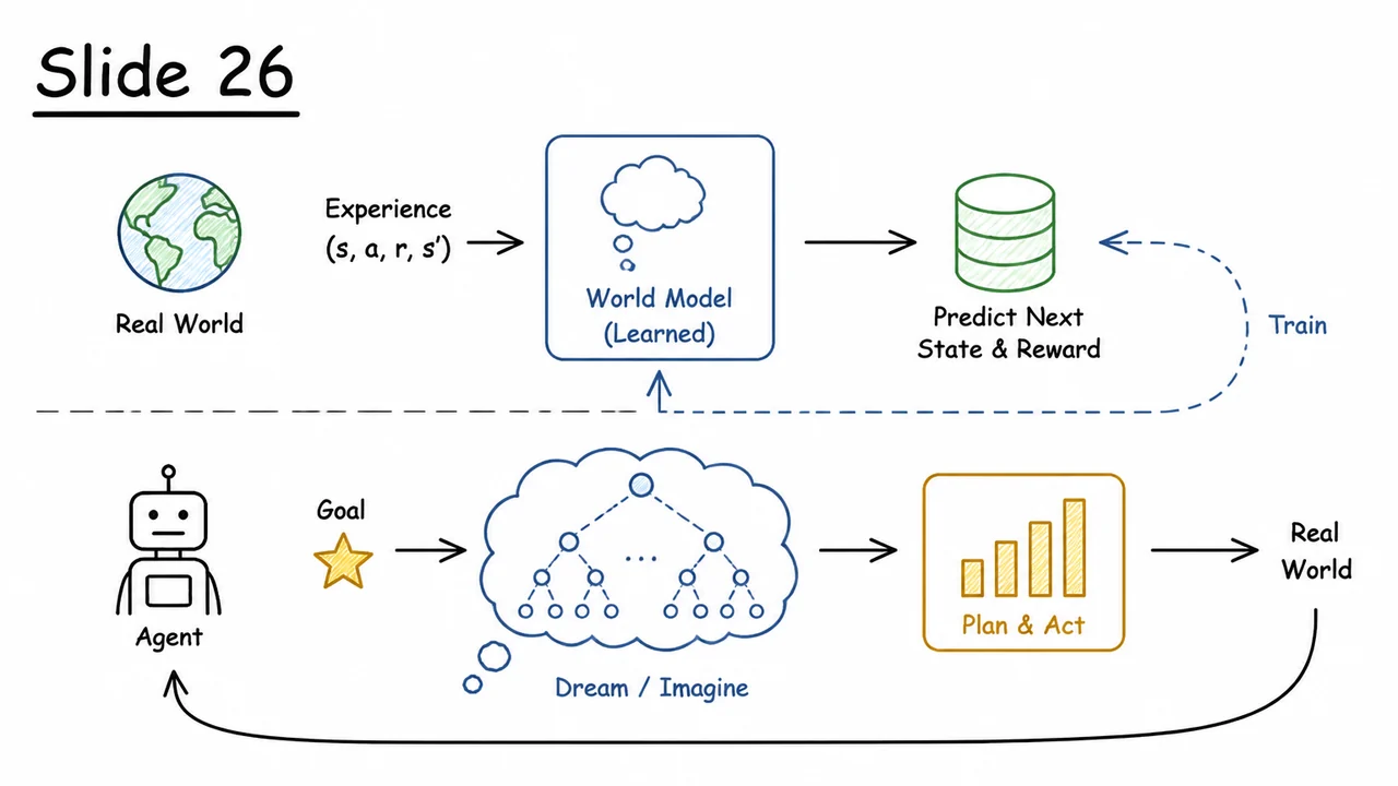
In the preceding sections, we walked through the full World Models pipeline, from the self-supervised compression of high-dimensional pixel observations down to the evolution-guided optimization of a compact controller. We saw that model-free reinforcement learning can be painfully sample-inefficient because it treats every raw frame as an independent data point, ignoring the underlying structure that could be reused across time. A world model attacks this problem head-on by learning to simulate the environment inside an agent’s “imagination,” so that the agent can practice thousands of virtual rollouts without ever touching a real simulator or a physical robot. The resulting architecture can be understood as three cooperating modules, each with a clear responsibility, a distinct loss function, and its own source of training data.
The first module is the variational autoencoder (VAE), which compresses each high-dimensional observation into a compact latent vector . Its encoder produces a distribution ; during training we sample from this distribution and reconstruct the observation through a decoder , but at test time we use the deterministic mean . The VAE is trained on a random collection of frames, independent of any action. The objective balances reconstruction fidelity against a prior-matching regularizer:
where typically . The hyperparameter controls the trade-off between sharp reconstructions and a smooth, structured latent space that the dynamics model can later navigate.
The second module is the mixture-density network recurrent neural network (MDN‑RNN), which learns to predict the next latent state given the current latent , action , and the RNN’s hidden state . Instead of a deterministic point estimate, the MDN‑RNN outputs the parameters of a Gaussian mixture model over the next latent vector. This stochasticity is essential: real environments are often non-deterministic, and even a perfect latent representation can contain irreducible uncertainty. The loss is the negative log-likelihood of the observed next latent sequence:
Training uses sequences of latent vectors obtained by first running the VAE encoder on recorded episodes, together with the actions that were taken. Importantly, the MDN‑RNN never sees raw pixels; it lives entirely in the learned latent space, which makes its training fast and its “dreamed” rollouts computationally cheap.
The third module is the controller, a small feed-forward or linear network that maps the concatenation of the current latent code and the RNN’s hidden state to a compact action vector . This controller is not trained by backpropagation through time on real rewards; instead, we treat it as an individual in a population optimized by evolution strategies (ES). In each generation, we sample perturbations of the controller’s parameters, let those perturbed agents run dream rollouts using the frozen VAE and MDN‑RNN, and evaluate their cumulative reward. The gradient estimate is then used to update the mean parameter vector:
This decoupling is profound: the representation is learned offline from raw pixels; dynamics are learned offline from latent trajectories; and the policy is learned completely inside the model’s “dream,” without any further interaction with the real environment. The result is a dramatic leap in sample efficiency.
At deployment time, the full loop is straightforward: encode the real observation to via the VAE encoder, feed the pair to the controller to obtain the next action , step the real environment, and simultaneously update the MDN‑RNN’s hidden state with the transition. Because the core computations—latent encoding, RNN forward pass, and controller forward pass—are all lightweight, the agent can run in real time, even on modest hardware.
Takeaways from this blueprint are worth highlighting.
The visual below consolidates these relationships into a clean quarter-column table. The Component column labels each module, while Output identifies its typical inference-time product. The Loss / Objective column presents the core mathematical form in the notation we’ve used throughout the lecture, and the Training Data column reminds us that each component lives on a different slice of the overall data pipeline. By absorbing these four rows—VAE, MDN‑RNN, Controller, and the integrated deployment loop—you can recover the entire World Models framework at a glance. The table does not replace the deeper derivations, but it serves as an essential cheat-sheet, making the theoretical scaffolding immediately accessible when you revisit the method or plan your own implementation. In that sense, it transforms a potentially sprawling set of equations into a single unified picture of how world models learn to dream, and why that dreaming makes reinforcement learning dramatically more efficient.
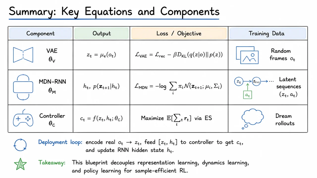
The journey through World Models has shown us that dreaming is not just a poetic metaphor—it is a computationally grounded strategy for overcoming the crippling sample inefficiency of model-free reinforcement learning. By systematically compressing raw high-dimensional observations into a compact latent code, learning a stochastic dynamics model over those codes, and then training a tiny controller entirely inside the self-generated dream, an agent can master complex continuous control tasks from pixels with orders of magnitude fewer environment interactions. Yet as satisfying as the full pipeline is when it works, the empirical successes on the CarRacing benchmark also illuminate subtle failure modes and open questions that have driven a wave of follow-up research.
At the heart of the World Models architecture lies a careful separation of representation, dynamics, and control. The variational autoencoder (VAE) learns to map each 64×64 RGB frame to a low-dimensional Gaussian latent vector and a reconstruction , trained to minimize the evidence lower bound:
A stronger pushes the posterior toward the unit Gaussian prior, encouraging a smoother latent manifold at the cost of reconstruction fidelity—a tension that becomes critical when small visual features, like the precise angle of a car’s front wheels, carry enormous control significance. After pre-training the VAE on random rollouts, the high-dimensional pixel space collapses into a compact code, and the agent no longer needs to reason about raw images again.
The MDN-RNN then models the temporal evolution of this latent space. Given the current latent and its own hidden state , it predicts a Gaussian mixture distribution over the next latent :
Training minimizes the negative log-likelihood of the actual next latent under this mixture, thereby learning a rich, multi-modal transition model that captures the inherent stochasticity of the environment—including the random perturbations and non-deterministic behaviours that are abundant in driving simulators. The hidden state acts as a recurrent memory, encoding the history needed to disambiguate partially observed situations.
With a perfectly pre-trained VAE and a well-fitted MDN-RNN, the dream world becomes a surrogate for reality. Training the controller now reduces to an optimization over a tiny parameter vector (often a linear layer or a single-hidden-layer network) that maps to an action . Because the transition model is differentiable, one could imagine backpropagating through imagined rollouts. However, the original World Models recipe uses evolution strategies (ES), a gradient-free black-box optimizer that adds isotropic Gaussian noise to , evaluates rollout returns, and moves the mean parameter toward higher-scoring perturbations. This choice neatly sidesteps the difficulty of credit assignment through an RNN over long horizons and works surprisingly well, albeit with high variance and modest sample complexity of its own.
On the CarRacing task, this recipe yields an agent that learns to navigate a winding track after only about 1,000 episodes of interaction—a tiny fraction of what conventional model-free algorithms require. The majority of the training happens entirely inside the dream, where the agent can experience thousands of imagined trajectories without a single new frame from the real simulator. This is the dream in action: the agent refines its controller in a fast, cheap, and safe internal world, occasionally checking its performance against reality to correct for any drift between the dream and the true dynamics.
However, CarRacing also exposes the brittleness of the approach. If the VAE’s latent representation discards subtle but crucial information (e.g., the precise curvature of a tight bend not well represented in the random rollout data), the controller can never recover because it simply does not have access to the necessary state. The MDN-RNN, while effective, is not infallible: small compounding errors in the latent predictions can lead to hallucinated situations that the controller overfits to, causing catastrophic failure when deployed back in the real environment. Moreover, training with ES becomes inefficient for larger policy networks or when the landscape of controller parameters is highly multimodal.
These limitations motivated the development of Dreamer and MuZero, which push the world-modeling paradigm further. Dreamer dispenses with the evolution strategies controller and instead learns an actor-critic agent purely inside the latent imagination, using imagined value estimates and policy gradients that flow through the recurrent state space model. This tighter coupling between the world model and the agent eliminates the need for a separate black-box optimizer and results in richer, more stable learning. MuZero takes a complementary path: it never reconstructs observations at all, instead learning a model that directly predicts future rewards, values, and policies. By abandoning pixel-level reconstruction, MuZero focuses representation capacity on quantities that matter for decision-making, achieving superhuman performance on Atari, chess, and Go with a unified architecture.
The accompanying diagram (Slide 28) captures this arc in a single visual abstraction. At its core, it shows the three canonical modules of the World Models pipeline—the VAE, the MDN-RNN, and the tiny controller—connected by arrows that signify the flow from raw pixels to actions through compressed dreams. Around it, sparse annotations mark the empirical triumph on CarRacing and the branching extensions represented by Dreamer and MuZero. The hand-drawn aesthetic strips away every unnecessary detail, leaving only the conceptual skeleton: compress, dream, act, and—crucially—remember that the dream must evolve when it begins to mislead.
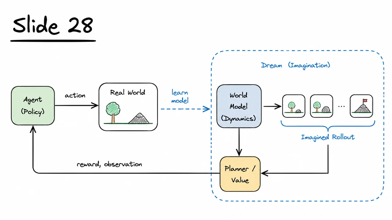
Imagine watching a reinforcement learning agent master an Atari game. After tens of millions of frantic frames — button presses, missed shots, pixel-level explosions — it eventually plays better than most humans. That’s the success story we hear about model‑free deep RL: a single network learns directly from raw pixels and rewards, turning a black‑box environment into a policy that acts. But behind the celebration lurks a sobering number. The canonical DQN (Deep Q‑Network) required ~200 million environment frames to surpass human‑level performance on a suite of Atari games. At 60 frames per second, that equates to roughly 38 days of continuous play. The agent does not share any of this experience across tasks; each new game forces the agent to start from scratch, burning another 200 million interactions just to rediscover the mechanics of paddles, bullets, or gravity.
This brute‑force requirement exposes the central weakness of model‑free RL: it treats the environment as a complete unknown and relies solely on trial‑and‑error to assemble a strategy. The agent’s mind has no internal representation of how the world behaves — no understanding that pushing right will move a paddle to the right, that a ball bouncing off a wall will reverse its trajectory, or that a specific enemy pattern repeats every few seconds. All such structural knowledge must be re‑extracted from raw data every time, leading to catastrophic sample inefficiency.
Contrast this with a human player. Give a person a new Atari game she has never seen, and within minutes — perhaps dozens to a few hundred actions — she grasps the objective, learns the basic controls, and starts achieving non‑trivial scores. She does not need to die ten thousand times to figure out that touching a monster is bad; a few observations and a quick mental model of cause and effect suffice. This ability to generalize from a handful of examples is often called one‑shot or few‑shot adaptation, and it is a hallmark of biological intelligence. The human brain constructs a compact internal simulator of the game’s dynamics, allowing her to plan tentative moves, predict outcomes, and transfer concepts like “avoid moving obstacles” or “collect shiny objects” instantly.
In reinforcement learning, we quantify this discrepancy with sample efficiency: the number of environmental interactions required to reach a target performance threshold. For many real‑world applications — robotics, autonomous driving, medical treatment design — collecting millions of trials is prohibitively expensive or dangerous. A robot cannot keep falling down thousands of times just to learn to stand. Therefore, the gulf between human‑level sample efficiency and model‑free RL’s hunger for data motivates a fundamental shift in how we build agents. The core insight is that an agent equipped with a learned model of its world can drastically reduce the interactions needed, because it can rehearse, plan, and “dream” inside its own simulator instead of always querying the real environment.
The problem with model‑free RL is not just the sheer volume of data; it’s the lack of transfer. Without an internal dynamics model, each new task demands massive re‑exploration, even if it shares underlying physics with a previously mastered task. The agent cannot say, “This game looks like the last one but with different colors; I’ll reuse my mental model of gravity and collision.” Every pattern must be rediscovered. A learned world model, on the other hand, captures the invariant causal structure of the environment, enabling rapid adaptation and, as we will see later, allowing the agent to compress experiences, generate imagined rollouts, and train a compact policy entirely within its own mind.
The visual below distills this contrast into a single glance. On the left, it draws a schematic of the model‑free loop: a labeled box for a Deep Q‑Network outputs an action into an opaque black‑box “Environment (Atari)”, which returns the next observation and a scalar reward . A stark counter reads “Frames: 200M,” and inside the agent’s box there is no internal structure beyond a generic “policy/value” node — a blind mapping from pixels to actions. On the right, the diagram shows a human figure beside a screen displaying a new, unfamiliar game; a thought bubble captures the rapid adaptation: “≈ 5 min adaptation.” The blue‑on‑red color scheme visually pits the slow, data‑guzzling model‑free approach against the fast, model‑rich human mind, making the argument for world models self‑evident.
This side‑by‑side layout immediately communicates why we need to move beyond model‑free methods. It hints at the solution: if we could replace the black‑box environment with a learned internal simulator, the agent could practice inside its own head and escape the tyranny of 200‑million‑frame trial‑and‑error. The rest of this lecture will show exactly how to build, train, and use such a dream‑capable world model.
The brute‑force approach of model‑free RL — learning a policy or value function entirely from live, high‑fidelity interaction — is extremely wasteful. Even the most sample‑efficient algorithms often require hundreds of thousands or millions of real environment steps to achieve competent behavior. This is not merely an engineering inconvenience; it fundamentally restricts reinforcement learning to domains where data is cheap or simulation is already perfect. The natural antidote is to give the agent the ability to build its own predictive simulator of the world. That shift, from experiencing to predicting, is the heart of model‑based reinforcement learning.
In model‑based RL, the agent learns an approximate world model of the environment’s dynamics. Rather than treating every transition as a black‑box surprise, the agent maintains two learned functions:
These approximations are trained on the same real interaction data the agent collects, but once they are reasonably accurate, they unlock a completely different mode of operation. The agent can now plan by unrolling its model many steps ahead, exploring imagined trajectories that never touch the true environment. Policy training can be carried out entirely inside this synthetic world, using virtually unlimited dream rollouts.
The sample efficiency advantage is stark. A single real transition can be used to train the model, and thereafter the model can generate thousands of simulated successor transitions at zero additional cost in real interactions. This decouples the agent’s learning from the environment’s interaction budget. Even crude early models can provide useful synthetic data that accelerates exploration or stabilizes policy updates. It is not an overstatement to say that model‑based methods trade real‑world samples for computation, a currency that modern hardware supplies in abundance.
Yet this elegant solution introduces a critical and insidious risk: model bias. Every transition model is an imperfect approximation of the true dynamics. When the agent plans or trains on imagined rollouts, small errors in a single‑step prediction compound multiplicatively over the rollout horizon. After a handful of imagined steps, the synthetic observations can drift into regions of state space that are either physically impossible or never encountered during real interaction. The policy, trained relentlessly on these flawed fantasies, learns to exploit the inaccuracies of the model rather than mastering the actual task. In the worst case, the agent discovers a policy that scores perfectly in the learned simulator but fails completely in reality. Controlling this compounding error is the central challenge of model‑based RL, and it is a theme that will recur in every section that follows.
The rest of this lecture takes model‑based RL into the high‑dimensional visual domain. Instead of trying to predict raw pixels directly — a task that is both computationally prohibitive and prone to catastrophic error accumulation — we will learn a compressed, latent world model. This enables a practical pipeline where a generative model (VAE) distills images into low‑dimensional features, a recurrent network (MDN‑RNN) models the stochastic dynamics of the latent state, and a compact controller learns to act within that imagined latent space. But before we dive into that architecture, it is worth pausing to visualize the qualitative difference between model‑free and model‑based loops.
The accompanying diagram makes the contrast immediately tangible. On the left, the familiar Model‑Free Loop shows an agent that interacts directly with a gray, opaque environment: actions are emitted, observations and rewards are received, and all learning must occur within that closed loop. The right panel — the Model‑Based Dream — introduces a blue World Model block that sits between the agent and the environment. The model first digests real transitions to learn and ; then a dashed Dream Rollout loop takes over. Instead of querying the real environment, the model re‑feeds its own predicted next observation (along with actions) into itself, generating an unlimited stream of synthetic data. The green Agent (Policy) block can now be trained using these dream trajectories, completely decoupled from the grey real world. The dashed blue arrow loop is the visual essence of the idea: learning to dream as a replacement for constantly asking reality for one more expensive step. This architectural split — real data for model training, synthetic data for policy training — is what makes sample efficiency possible, while the accumulating error in the dashed loop is the silent threat we must now learn to contain.
Having established that model-based reinforcement learning can plan with a learned simulator, a natural question arises: can we directly apply these ideas to environments with high-dimensional observations, like raw pixels from a racing game? In theory, yes – we could train a transition model that predicts the next frame of pixels. In practice, raw pixel prediction is both computationally expensive and unreliable: small errors accumulate, the model often blurs details or produces implausible hallucinations, and planning through such a flawed model quickly diverges. The Dream Hypothesis, introduced by Ha and Schmidhuber (2018), elegantly sidesteps this problem by separating perception and dynamics from the decision-making policy, and training the latter entirely inside a learned dream.
The core insight is to decompose the agent into a large, pre-trainable World Model and a compact Controller. The world model’s job is to compress high-dimensional observations into compact, meaningful latent representations and to learn the stochastic dynamics that govern transitions between these latent states. The controller, on the other hand, is a small, focused network that takes latent features (and possibly some recurrence) as input and outputs actions – it never sees a raw pixel. Crucially, the controller is trained exclusively inside the world model’s imagination, not by interacting with the real environment. This architecture shifts the heavy computational burden to an offline pre-training phase, where the world model learns to dream plausible futures from unlabeled experience, while the controller remains lean and can be optimized efficiently with only simulated rollouts.
Two components form the World Model. The first is a Variational Autoencoder (VAE) that maps each high-dimensional observation (e.g., a screen frame) to a low-dimensional latent code . The VAE is trained to reconstruct the original observation, encouraging to capture essential structure while discarding irrelevant pixel-level noise. The second component is a Mixture Density Network combined with a Recurrent Neural Network (MDN-RNN). This network takes the current latent state , the action , and an internal hidden state that summarizes the history, and outputs the parameters of a Gaussian mixture distribution over the next latent state and reward:
The MDN-RNN thus captures the stochastic dynamics and intrinsic uncertainty of the environment in the compact latent space. Because the VAE decoder is still available, the world model can – if desired – render a dream observation:
However, the controller does not need to see these pixel reconstructions; it only relies on the latent codes and rewards.
Pre-training of the world model is remarkably flexible. The VAE and MDN-RNN can be trained on unlabeled random rollouts, for example from a random agent or even from a human demonstrator, without any reward maximization in mind. This means we can collect a dataset of transitions purely for the purpose of learning to imagine, and the world model learns to hallucinate plausible environment dynamics independent of any specific task. Once trained, the world model can generate an endless stream of “dreamed” rollouts: starting from an initial latent state and hidden state , the model repeatedly samples and conditioned on the current action. These dreamed trajectories contain all the information the controller needs: latent states and rewards.
Training the controller inside the dream then becomes a black-box optimization problem. Because the controller operates on a low-dimensional latent input and the dream dynamics are differentiable in principle, one could use gradient-based methods. The original World Models paper, however, employed Evolution Strategies (CMA-ES) to optimize the weights of a compact linear policy directly for cumulative dreamed reward, completely circumventing the need to backpropagate through time or through the world model. This separation allows the controller to be extremely small, sometimes containing only a few hundred parameters, and yet achieve competitive performance when deployed in the real environment.
A remarkable demonstration of the dream hypothesis comes from the CarRacing environment. After pre-training the world model on random rollouts, an agent was trained entirely inside the dream, evaluating thousands of simulated episodes without ever seeing a real frame during the controller’s training. When transferred to the real game, this purely dreamed-up policy achieved competitive lap times, validating that the hallucinated environment was sufficiently realistic. The visual below juxtaposes a real frame from CarRacing on the left with a dream-generated frame on the right, connected by an arrow labeled “Dream”. The dream image, though slightly blurry, retains the structure of the winding road, the red car, and the surrounding grass – enough for a controller to learn effective steering and acceleration. A caption reinforces the key claim: the agent trained entirely inside the dream never sees the real environment during training. This image serves as both a conceptual summary and a piece of empirical evidence that dreaming can replace real interaction for policy learning, provided the world model is capable of faithful reconstruction and dynamics modeling. In the following sections, we will formalize the objective functions for the VAE, the MDN-RNN, and the controller, and examine how later frameworks like Dreamer and MuZero built upon this dream hypothesis.
The leap from dreaming to a rigorous problem statement requires us to ground the conversation in the formal language of reinforcement learning. In model‑free deep RL, an agent learns a policy that directly maps high‑dimensional observations to actions by sampling millions of environment transitions. This is profoundly sample‑inefficient: every pixel of every frame is processed essentially as raw data, and no internal model of the world ever emerges. The agent cannot mentally simulate “what would happen if” without actually executing the action in the real environment. The dream hypothesis (Ha and Schmidhuber, 2018) proposes a deceptively simple alternative: learn a compressed generative model of the environment, then train a compact policy entirely inside that learned dream. To make this precise, we need a shared notation and a clear decomposition of the learning pipeline.
We treat the environment as a partially observable Markov decision process (POMDP) with high‑dimensional observations. At each discrete time step , the agent receives an observation – for instance, an RGB frame from a video game – and must select an action . The environment then returns a scalar reward and transitions to the next observation . The true underlying state of the environment (the exact physics, object positions, velocities) is not directly visible; the agent sees only the pixel matrix. The objective, as in standard RL, is to maximize the expected cumulative discounted reward from the start to a terminal time :
where is the discount factor. When is a high‑dimensional sensory stream, directly optimizing via model‑free methods like policy gradients or Q‑learning demands an enormous number of real interactions because the policy must implicitly learn a perception system, a state representation, and a value function all at once.
The World Models blueprint circumvents this by factorizing the problem into three learned modules, each with its own parameter set and training schedule. The first module, a vision encoder (typically a variational auto‑encoder, VAE), maps the raw observation to a compact latent vector . This step discards irrelevant detail while preserving the information needed to predict future frames. The VAE is trained offline on a dataset of collected frames, learning parameters that define both the encoder and the decoder (the decoder is used only to verify reconstruction quality and is not part of the dreaming loop).
The second module is a memory‑based dynamics model. Because the environment is partially observable, the latent vector alone may not contain enough information to predict the future. The model therefore maintains a recurrent hidden state that summarises the entire history . The dynamics model, parametrised by , is a Mixture Density Network combined with an RNN (MDN‑RNN). At each step it takes the previous hidden state , the current latent , and the action to produce the new hidden state, a prediction of the next latent , and a prediction of the reward :
The MDN component outputs a Gaussian mixture distribution over , capturing the stochasticity of real‑world transitions and making the dreamed rollouts more robust. The reward prediction is typically a single scalar head. Training the dynamics model requires sequences of collected by running a random policy or the current controller in the real environment; the MDN‑RNN is then optimised by maximum likelihood.
The third module is the controller, parametrised by . It is a simple policy – in the original work, often just a linear model – that maps the concatenation of the latent state and the memory state directly to the action: . Crucially, the controller is not trained on real environment trajectories. Instead, it is optimised entirely inside the learned dream: the world model (VAE + MDN‑RNN) is frozen, and the controller is tasked with maximising the cumulative dreamt reward. Because the world model is fully differentiable only with respect to the controller’s inputs, evolution strategies (e.g., CMA‑ES) or other black‑box optimisation methods are used to update without requiring backpropagation through the whole model.
This three‑way decomposition – for perception, for dynamics and memory, for behaviour – is the conceptual engine behind the approach. It separates representation learning from forward prediction and from decision making, allowing each component to be trained with a method suited to its role. The VAE learns a compressed space, the MDN‑RNN learns to roll out and evaluate imagined trajectories, and the controller learns a task‑specific policy without ever seeing a real pixel again after the initial data‑gathering phase. By dreaming, the agent can simulate thousands of episodes per second, radically reducing sample complexity.
The visual that accompanies this section distills the full problem formulation into a single, glanceable architecture. It begins with a narrow box representing the raw POMDP loop – the flow of , , and – and places the central objective prominently below it. Then, in a horizontal row, three colour‑coded modules appear: a blue encoder compressing into ; a green memory‑dynamics block taking , , and to produce , , and ; and an orange controller mapping to the next action. Beneath each module, the corresponding parameter symbols , , and are shown, reinforcing that the world model is not one monolithic network but a carefully composed ensemble. This diagrammatic summary makes the abstract notation concrete: the reader can see at a glance how perception, imagination, and action are welded together into a system that learns to dream before it learns to act.
The previous section framed reinforcement learning as a sequential decision problem—an agent interacting with an environment to maximize long‑term reward—and established the notation for observations, actions, states, and trajectories. In principle, we could solve such problems with model‑free algorithms that directly map pixels to actions through deep networks, and indeed spectacular results have been achieved this way. Yet anyone who has trained a DQN or PPO agent on a visually rich environment knows the pain: millions of environment steps, painfully slow wall‑clock times, and fragile policies that collapse when the reward signal becomes sparse or deceptive. The root cause is sample inefficiency. Model‑free methods treat the world as a black‑box oracle that must be queried for every single scrap of experience, and they rarely share that experience across tasks or can re‑use the underlying dynamics for anything else.
The world models approach turns this on its head. Instead of discarding the environment after each interaction, we learn a compressed, predictive model of it. The idea is elegant: the agent first builds an internal “dream simulator” of the environment’s dynamics in a compact latent space, and then trains its policy almost entirely inside that dream. The real environment is still needed, but only occasionally, to ground the dream in reality. In this way, we replace expensive physical interaction with cheap, parallelizable simulated rollouts—while preserving the essential causal structure of the problem.
To see how this is possible, consider what an agent truly needs from a high‑dimensional observation like a game frame. A 96×96×3 image contains over 27,000 numbers, but the information that matters for decision‑making—the position of the car, the curve ahead, the velocity—likely lives on a manifold of much lower dimension. If we can learn a mapping that compresses each raw observation into a small latent vector which faithfully captures the task‑relevant state, we can then model the environment’s dynamics using only these latent codes. Formally, we want a generative model that captures and a recognition model (encoder) that approximates ; that is precisely what a Variational Auto‑Encoder provides.
But compression alone is not enough. We also need to know how evolves in response to actions. If we attempted to model the transition with a deterministic function, we would quickly be disappointed: the real world, and even many simulated environments, contain stochastic elements (e.g. random track textures, friction variability, or noisy actuation). The next latent state is better described by a mixture of Gaussians, whose parameters depend on the current latent state, the action, and also on a hidden memory state that accumulates information over time. An MDN‑RNN (Mixture Density Network combined with a recurrent neural network) fits this role naturally: the RNN maintains a deterministic hidden state that integrates past experience, and at each step the MDN head outputs the parameters of a Gaussian mixture that models the distribution of and possibly the reward . The model is trained by maximizing the likelihood of real trajectories observed so far.
With the VAE compressing observations and the MDN‑RNN predicting future latent encodings, we have the core of a world model. The third component is a compact controller that maps the concatenation directly to an action . Because the latent representation is small and the dynamics model is differentiable (or can be treated as a black‑box simulator), we can train the controller without back‑propagating through the visual encoder. The original Ha and Schmidhuber paper used evolution strategies (ES) for this final step: they perturb the controller’s weight vector, run many imagined rollouts inside the world model, and keep perturbations that lead to higher total dreamt reward. That strategy is simple, parallelizes across CPU cores, and avoids credit‑assignment issues that often plague long imagined trajectories.
This separation into three trainable modules—a visual encoder, a latent‑space dynamics model, and a controller—is what gives the world model its power and its name. Once the VAE and MDN‑RNN have been trained on a modest set of real transitions, the agent can dream: it starts from the latent encoding of a true frame and then, for hundreds of steps, feeds its own predicted back to the RNN, collecting simulated rewards, all without ever rendering a pixel or touching the real environment. Training the controller inside this dream is not only faster; it also decouples the policy search from the slow, serial process of real‑world interaction.
The visual below captures this entire pipeline in one coherent diagram. It shows the three modules—VAE, MDN‑RNN, and controller—connected by arrows that trace the flow of information. On the left, a high‑dimensional observation passes through the VAE encoder to become a compact latent . That latent, together with the previous hidden state and action , feeds into the MDN‑RNN, which updates its hidden state to and predicts the parameters of a mixture distribution over the next latent state and, optionally, the reward. The controller takes the concatenation and outputs the next action . A dashed loop indicates the “dream” mode: the model can run autonomously by replacing the real with a sample from the MDN‑RNN’s predicted distribution, enabling long simulated rollouts. Hand‑drawn annotations and muted colors—blue for the VAE, amber for the MDN‑RNN, green for the controller—help the reader instantly separate responsibilities while seeing how they cooperate to form the full world model.
Reinforcement learning agents that operate directly on raw sensory inputs—pixels from a game frame, for example—face a punishing sample inefficiency. Learning a value function or a policy from high-dimensional observations without any prior structure can require millions of environment steps, most of which are spent rediscovering the same basic visual features. The World Models framework attacks this problem by decomposing the agent into a large world model that learns a compressed, predictive representation of the environment, and a compact controller that acts within that learned representation. The heavy lifting is done by the world model, which is trained offline and can even “dream” simulated experience, relieving the controller from having to reconstruct the world from scratch every time it makes a decision.
The first pillar of this world model is a vision module whose job is brutally simple: take a high-dimensional observation (say, a 64×64 RGB frame) and compress it into a low-dimensional latent vector that preserves only the information relevant to solving the task. If this compression works well, then all downstream learning—predicting future latents, training the policy—happens in a space that is orders of magnitude smaller and where geometric relationships are much easier to model. The chosen tool is a Variational Autoencoder (VAE), which provides a principled probabilistic framework for learning such a compact latent code.
A VAE models the generative process that produces observations from latent codes, together with an approximate posterior that acts as an encoder. In the World Models implementation, both the encoder and decoder are neural networks parameterized by . The encoder outputs the parameters of a diagonal Gaussian distribution over the latent variable: Sampling from this distribution via the reparameterization trick yields a stochastic that can be passed through the decoder to reconstruct the observation. The choice of a stochastic encoding is essential: it provides a natural way to inject noise and uncertainty, and it regularizes the latent space so that nearby points decode to visually similar frames, which in turn helps the next component—the dynamics model—operate smoothly.
To train the VAE, we maximize the Evidence Lower Bound (ELBO) on the log-likelihood of the observed data, but with a crucial modification—a scalar that scales the KL divergence term: The first term is the reconstruction log-likelihood; for pixel data it is often a Gaussian likelihood with fixed variance (equivalent to an L2 loss) or a Bernoulli likelihood (binary cross-entropy). The second term pulls the approximate posterior toward the prior . When we recover the standard VAE; larger values of push the model toward a -VAE that encourages disentangled factors in the latent space, and smaller values trade off reconstruction fidelity for a weaker prior penalty. In the World Models paper, is tuned to balance latent capacity against reconstruction quality, though the primary aim is still to get a compact, usable representation for the dynamics model rather than perfectly disentangled features.
Importantly, the VAE is trained once on a dataset of observations collected by a random agent interacting with the environment, and then its weights are frozen. The encoder becomes a fixed perceptual module; every subsequent step of world-model learning or controller optimization simply calls the encoder to produce from the current . This design choice has profound implications. On the positive side, it decouples representation learning from policy learning, making training far more efficient—the controller never has to worry about high-dimensional vision. On the negative side, the VAE’s world representation is only as good as the random data it has seen. If the random rollouts never visit parts of the state space that a good policy would later require, the representation will have blind spots. Realigning the world model later or updating the VAE online are natural extensions to address this.
What goes into the latent ? The VAE is encouraged to discard pixel-level details that are irrelevant for control—like background textures, sky gradients, or tiny fluctuations—while retaining crucial spatial structure: the position of the car, road boundaries, obstacles, and their relative velocities. Because the VAE is probabilistic, the latent itself becomes a compact, smooth summary that already starts to abstract away the raw sensory stream. The visual that follows consolidates this whole pipeline: it shows the encoder mapping to a mean and variance, the sampling step to obtain , and the decoder reconstructing . The central display equation for the ELBO encapsulates the training objective, and the parameter is highlighted to remind us that its weight controls the trade‑off between faithful reconstruction and a well‑shaped latent prior. With the VAE in place, we can now turn to the second component—a dynamics model that learns to predict the next latent state given and the action —and begin to “dream” in this compressed space.
Having compressed each high-dimensional frame into a compact latent representation with the VAE, we now face a deeper challenge: the environment doesn’t just deliver a static picture—it evolves in response to actions, often in stochastic ways. Model-free RL learns this evolution implicitly through value functions or policy gradients, but it requires an immense number of environment interactions because it must rediscover the consequences of actions from scratch every few updates. The World Models architecture addresses this by learning an explicit dynamics model in the latent space that can be used to simulate trajectories without ever rendering pixels. This is where the Memory Module, the MDN-RNN, becomes essential.
At its core, the MDN-RNN is a recurrent neural network that takes the current latent state and action , along with its own previous hidden state , and produces a new hidden state . That hidden state serves two purposes: it acts as a compressed memory of the episode history so far, and it parameterizes a predictive distribution over the next latent state . The recurrence is crucial because the true future of an environment depends not just on the current observation and action but on unobserved aspects like velocity, momentum, or hidden intentions of other agents—information that can only be accumulated over time. The RNN (typically an LSTM or GRU) ingests the concatenation of and , along with , and outputs , which becomes the internal belief state for the next step.
What makes the MDN-RNN special is that it does not output a single deterministic prediction for . Instead, it models the environment’s stochasticity with a mixture density—a weighted sum of Gaussian distributions whose parameters are functions of the hidden state. The output layer transforms into three sets of vectors: the mixing coefficients , the means , and (typically diagonal) covariance matrices for each of mixture components. Then the probability density of the actual next latent state is given by
The softmax over the ensures these weights sum to one, while the means and variances give location and spread of each component. This construction is a natural choice for world models because many real-world transitions are multi-modal: from the same state and action, several distinct futures might be possible. For example, when the agent drives a car toward an intersection, the next state could be a left turn or a right turn, not a smooth average of both. A single Gaussian would place its mass in the middle, predicting an impossible blend; the mixture can assign separate peaks to each plausible outcome.
Training the MDN-RNN is a straightforward supervised learning problem: we collect a large dataset of trajectories by running a random or preliminary policy in the environment, encode every frame with the frozen VAE to obtain the sequence of latent vectors , and then optimize the network parameters to maximize the likelihood of each actual next latent state given the history. This translates into minimizing the negative log-likelihood over all time steps:
Notice that the targets are the VAE’s compressed representations—real vectors, not discrete tokens—so the mixture density deals with continuous latents. Because the VAE itself is stochastic, the latents already carry some noise, and the MDN learns to absorb that uncertainty into its predictions. A common practical choice is to use diagonal covariances , which keeps the number of parameters manageable and makes the log-density calculation efficient, while the multiple components still capture complex shapes through overlap.
An important subtlety is that the RNN and the mixture-density heads are trained jointly end-to-end. The hidden state is not just a summary of past observations; it is shaped by the learning signal that flows back from the prediction errors on future latent states. This means the network learns to extract exactly the temporal features that are useful for forecasting, often discovering dynamics-related invariants like velocity or acceleration without any explicit supervision. Once trained, the MDN-RNN can simulate in latent space: at each step, we sample a from the predicted mixture, feed it back as the next input together with the action, and continue the dream.
The visual below consolidates this architecture into a single flowing diagram. On the left, three incoming signals— (the current VAE latent, colored orange), (action, blue), and the recurrent hidden state (gray)—enter a central LSTM/RNN block, which outputs the updated . From that hidden vector, three parallel fully connected layers branch out: a softmax layer producing the mixture weights , a linear layer producing the component means , and another layer producing the (diagonal) log-variances . These three groups of parameters feed into a rounded box labeled “Gaussian Mixture Model ”, from which an arrow points to the predicted next latent . Beneath the diagram, a concise caption reminds us that the whole module is trained by minimizing the negative log-likelihood of the actual VAE latent from recorded rollouts. The diagram matches exactly the step-by-step computation we’ve just described, making the interplay between recurrence, mixture modeling, and training signal immediately apparent.
Having designed an RNN that can forecast future latent states, we hit a more fundamental question: how do we get from raw pixels to the compact, information-dense representations that the dynamics model needs? World Models answers this with a variational autoencoder (VAE), a generative model trained to compress high-dimensional observations into a low-dimensional latent space while retaining enough detail to reconstruct the original frame. The VAE’s objective is not a simple reconstruction loss but a principled lower bound on the log-marginal likelihood of the data, a derivation that sits at the heart of modern latent-variable modeling.
We begin by writing the marginal likelihood of an observation under a latent variable model with prior and likelihood . Dropping the time index for clarity, the log-marginal is
The integral over the latent space is generally intractable—we cannot enumerate all configurations for a high-dimensional image. The standard trick is to introduce an approximate posterior distribution , often called the encoder, and use it to rewrite the log-likelihood. By adding and subtracting the KL divergence between and the true posterior , we obtain
Since the KL divergence from the approximate to the true posterior is always non‑negative, dropping it yields a lower bound—the Evidence Lower Bound (ELBO):
This inequality crystallizes the VAE’s learning problem. The first term, the expected log-likelihood under the encoder’s samples, pushes the decoder to faithfully reconstruct the observation—for images, it boils down to per‑pixel Gaussian log-likelihood (MSE) or Bernoulli cross‑entropy. The second term, the KL divergence between the encoder’s output distribution and the prior , acts as a regularizer that pulls the latent representations toward a simple distribution, typically a standard Gaussian. The bound is tight exactly when equals the true posterior, so optimizing the ELBO encourages both accurate reconstruction and a well-structured latent space.
In practice, we often use a -VAE, where a coefficient scales the KL term:
When we recover the standard ELBO. Increasing enforces a stronger bottleneck, which can improve disentanglement of latent factors at the cost of reconstruction fidelity. For World Models, a moderate helps keep the latent codes compact and stationary, an ideal substrate for the MDN‑RNN to model over time.
A huge practical advantage of the VAE objective is that the KL term has a simple closed form under Gaussian assumptions. We choose the prior and let the encoder output the mean and variance for each dimension of a diagonal‑covariance posterior . Then the KL divergence becomes
This formula is purely arithmetic, so the loss is differentiable and cheap to compute. The reconstruction term is approximated by drawing one or more samples and using the reparameterization trick to backpropagate through the sampling step. The entire VAE is then trained end‑to‑end on a corpus of randomly collected frames from the environment—no reward signal needed.
The resulting latent vectors are low‑dimensional, continuous, and relatively smooth, which is exactly what the MDN‑RNN expects. Because the VAE is trained to maximise the ELBO, the latent space naturally captures the essential visual content while discarding irrelevant pixel‑level noise. This compression is what makes it possible to run the dynamics model thousands of steps ahead in a simulated dream, generating imagined trajectories that are both realistic and computationally cheap.
The visual below condenses these ideas into a clean reference. At the top, it shows the intractable marginal likelihood integral, emphasizing why a direct approach fails. A centered box then displays the core ELBO inequality: reconstruction expectation minus the KL penalty. Just beneath that, the -VAE loss is written out, underscoring the capacity‑control lever. Finally, the closed‑form KL divergence is given as a summation over dimensions, providing a ready‑to‑implement formula for the Gaussian case. In one glance, the diagram captures the mathematical flow from intractable marginal to trainable objective—a compact cheat sheet for the VAE component of World Models.
After mastering the VAE that squeezes high‑dimensional pixel frames into compact latent vectors, we face the next question: how does the world actually move from one state to the next? A static autoencoder gives us a useful alphabet, but efficient reinforcement learning requires a compressed forward model that can predict future latent states and rewards without looking at the raw sensory stream every time. This is precisely where the World Models architecture introduces its second component: a dynamics model trained entirely in the latent space of the VAE, typically realised as a Mixture Density Network combined with a recurrent neural network (MDN‑RNN).
The intuition is straightforward. An uncompressed environment frame (say, a image of a car racing track) contains far more detail than we need for planning. The VAE’s encoder already collapses this into a compact stochastic code . If we now observe a sequence of frames , we can compress each frame into a posterior sample and then train a recurrent network to predict the next latent state and the immediate reward given the history of previous latents and actions. Crucially, the MDN‑RNN does not output a single crisp prediction; it outputs a full probability distribution over the next latent vector. Since the latent space is itself stochastic (the VAE’s sampling step injects noise), a multimodal or heteroscedastic distribution is often needed. A Gaussian mixture model gives the network the flexibility to capture several plausible futures – for example, the car might continue straight or begin to swerve on a curve.
The training loss for the MDN‑RNN is simply the negative log‑likelihood of the observed next latent vector under the predicted mixture density, summed over time:
where is the RNN’s hidden state summarising previous latents and actions, are the mixing coefficients, and the network outputs all parameters of the Gaussians. A parallel head can predict the reward with a simple squared error or cross‑entropy loss if rewards are discretised. Because the dynamics model only sees the compressed latents and a continuous‑action input (e.g., steering and acceleration), it is orders of magnitude smaller than a pixel‑space predictor and can be rolled out for thousands of imagined steps in mere milliseconds.
Once the VAE and the MDN‑RNN are in place, we effectively possess a dream simulator: we can feed it an initial latent state and a sequence of actions, and it will hallucinate a chain of latent states and rewards. This dream world becomes the exclusive training ground for the controller – a small policy network that maps a latent state (and optionally the RNN hidden state ) directly to an action vector. Because the world model is fully differentiable or at least queryable at high speed, we can bypass traditional backpropagation‑through‑time limitations and instead use evolutionary optimisation, such as CMA‑ES (Covariance Matrix Adaptation Evolution Strategy), to search for controller weights that maximise the cumulative dream reward over many pseudo‑episodes.
The overall training pipeline thus consists of three stages that are repeated iteratively:
This decoupling is the core efficiency gain: the RL agent learns to imagine millions of steps per second, while only interacting with the true environment to occasionally update its world model. As a result, World Models achieved competitive scores on the CarRacing‑v0 benchmark using fewer than 1000 real episodes, a fraction of what model‑free methods require. The real genius is that the policy is never directly exposed to the original high‑dimensional observation; it lives entirely in the compact, abstract space learned by the VAE.
The visual below (or on the companion slide) consolidates this complete loop. It shows the three neural components – VAE encoder, MDN‑RNN, and controller – as hand‑sketched boxes arranged in a cycle: real frames enter the VAE to produce latents, the latents feed the MDN‑RNN which predicts future latents and rewards in a dream loop, and the controller receives latents from either the real world or the dream to output actions. Arrows indicate the flow of information and the distinct training signals (reconstruction loss for the VAE, next‑latent likelihood for the MDN‑RNN, and cumulative reward for the controller). By presenting the pipeline as a single diagrammatic snapshot rather than three separate slide bullets, the visual helps the learner instantly grasp how compression, dynamics, and policy co‑evolve in the World Models framework – a perfect summary before we turn to empirical results, failure modes, and the extensions that grew into Dreamer and MuZero.
Model-free reinforcement learning—where an agent learns a policy or value function directly from raw interaction with an environment—has produced remarkable results on tasks from board games to robotic control. Yet its appetite for data is staggering. An agent that learns to play Atari games from pixels may require tens of millions of frames; a simulated robot learning to walk can consume days of compute. This sample inefficiency stems from a fundamental reliance on trial-and-error in the high-dimensional, noisy space of sensor readings. Every new environment demands the agent to relearn even simple regularities—like the fact that objects persist when they leave the frame—from scratch through a deluge of episodes. The promise of world models is to break this dependency by giving the agent an internal, compressed imagination it can use to simulate experience, dramatically cutting the number of real interactions needed.
The core idea is simple and beautifully recursive: if we can learn a model that predicts how the world behaves given an action, then the agent can “dream” plausible futures and plan or train a policy inside its own mind. In the seminal World Models paper by Ha and Schmidhuber, this is achieved with three cooperating components: a Variational Autoencoder (VAE) that compresses high-dimensional observations (e.g., game frames) into a compact latent vector, a Mixture Density Network combined with a Recurrent Neural Network (MDN-RNN) that models the stochastic dynamics of the latent state over time, and a compact controller that maps the latent state and the RNN’s hidden state to actions. The controller is kept deliberately small—often a linear model or a shallow neural net—so that it can be trained efficiently, even with black-box optimization methods like Evolution Strategies (ES). The magic is that once the VAE and MDN-RNN are trained, the controller can be optimized entirely inside the learned “dream” world, requiring zero additional real experience.
Let’s unpack the compression step. When observations are high-dimensional, like 64×64 RGB images, it is hopeless to model raw pixel dynamics with enough fidelity to roll out realistic simulations. The VAE solves this by learning a probabilistic mapping from the observation space to a low-dimensional latent space that captures the essence of the scene. A VAE consists of an encoder network that outputs the parameters of a distribution (usually a diagonal Gaussian) and a decoder network that reconstructs the observation from a sample of that distribution . Training minimizes a loss with two antagonistic terms: a reconstruction loss that encourages faithful decoding, and a KL divergence that forces the latent distribution to be close to a simple prior —typically . This yields the evidence lower bound (ELBO):
where balances compression fidelity. By setting (a β-VAE), the model is pushed to learn more disentangled, robust latent representations that later benefit the dynamics model. In the CarRacing environment, this compresses an image into a vector of merely 32 or 64 numbers, preserving the track layout, car orientation, and relevant visual cues while discarding irrelevant pixel-level noise.
With a compact latent space in hand, the next challenge is capturing how the environment evolves. A deterministic model would be fragile because many real-world (and even simulated) dynamics are unpredictable: for instance, a car’s behavior on a curve may depend on subtle friction or random perturbations. The MDN-RNN addresses this by predicting a distribution over the next latent state given the current latent , the RNN’s hidden state , and the action . More precisely, the network outputs the parameters of a mixture of Gaussians—weights , means , and standard deviations —so that the conditional density is
The MDN-RNN is trained to maximize the log-likelihood of the observed sequence of latent states (produced by the frozen VAE encoder) given the actions. Additionally, it predicts the immediate reward from the same hidden representation, using a mean-squared error loss. This multi-task objective encourages the hidden state to accumulate information about the history that is useful for both state transition and reward prediction.
The stochasticity modelled by the mixture of Gaussians turns out to be crucial: it allows the agent to dream varied, plausible futures rather than a single deterministic hallucination, which in turn produces a controller that is robust to the sorts of surprises the real environment might throw at it.
Finally, the controller. Given that the VAE and MDN-RNN are pre-trained on rollouts from a random policy (or gradually improved upon), the controller learns to act purely inside the dream. It receives the latent state and the RNN hidden state and outputs the action . Because the input space is small and the dynamics are already captured by the RNN, the controller can be tiny—a single linear layer with a activation, for instance. Training this controller using Evolution Strategies (ES) is elegantly sample-efficient within the dream: we simply sample perturbations of the weight vector, run hallucinated rollouts with the MDN-RNN, and keep the weights that maximize cumulative reward. No backpropagation through time is required, and the method is trivially parallelizable. The result is an agent that can solve complex tasks like CarRacing with orders of magnitude fewer real environment steps compared to model-free baselines.
The visual below brings these three components together into a coherent pipeline. High-dimensional observations are funneled through the VAE’s encoder into a tiny latent code ; the MDN-RNN takes that code alongside its own hidden state and the action to predict the next and the reward; the controller, seeing only and , produces the next action. The entire loop—encode, predict, act—runs either on real frames or on dreamed ones, with the dashed boundary indicating the “world model” that isolates the agent from the expensive real environment. It shows how compression and learned stochastic dynamics become the engine of efficient reinforcement learning, a template that later works like Dreamer and MuZero would refine and extend. Keep this architecture in mind as we now dive into the specific VAE compression on CarRacing.
The previous section established the VAE as a principled way to learn a compact latent representation of high-dimensional observations. Now we see exactly how that abstraction earns its keep in the CarRacing-v0 domain, where every raw frame is a tensor—12,288 pixel values—that arrives at 60 Hz. If we naively fed those frames into a dynamics model, the sheer dimensionality would be prohibitively sample-inefficient, and much of the signal (grass textures, cloud patterns, minute colour fluctuations) carries no information about controlling the car. The first component of the World Models architecture therefore trains a -VAE as an information bottleneck that crushes this high-dimensional stream into a 32‑dimensional latent vector , discarding everything that does not help reconstruct the dominant scene structure.
Training the VAE does not require expert demonstrations or even a partially trained policy; it is performed entirely on random rollouts—frames collected by an agent taking uniformly sampled steering, acceleration, and brake actions. This is a critical design choice: the VAE never sees optimal driving, so it cannot accidentally encode a prior about “good” trajectories. Instead, it learns to represent the visual manifold of the environment itself, purely from the statistics of the image distribution. The loss function is the standard -VAE objective with :
The first term is the reconstruction log-likelihood—how well the decoder can recover the original frame from the sampled latent code. The second term is the KL divergence between the encoder’s distribution and a standard Gaussian prior, which acts as a regularizer that pushes the latent representation toward a smooth, continuous latent space. With (the classic VAE), this penalty is just strong enough to prevent the model from memorizing fine textures and pixel noise; the optimal solution balances accurate reconstruction of macroscopic geometry against a compact, well‑organized latent manifold.
The effect of this trade‑off becomes immediately visible in the reconstructions. When the VAE is asked to encode and decode a frame, the output is blurry: high‑frequency details like the rippling grass, the dithering of the sky gradient, and the tiny speckles of road texture are smoothed away. Yet the essence of the scene remains sharp: the road boundaries, the position of the horizon, the silhouette of the car, and the upcoming curves are all faithfully preserved. This is not a failure of the model but precisely the intended behaviour—the model has learned that those high‑frequency niceties are irrelevant for predicting itself under random jitter, and so the latent code devotes its limited 32 dimensions to capturing only the task‑relevant structure. In information‑theoretic terms, the VAE discards the “noise” that would otherwise drown the dynamics model in irrelevant variance.
Why is this blurring a feature, not a bug? The RNN that will learn the environment’s dynamics (the MDN‑RNN) now operates on vectors of 32 numbers instead of 12,288. Reducing the dimension by a factor of nearly 400 makes the prediction task dramatically easier, requiring orders of magnitude less data to converge. Moreover, the information bottleneck acts as an implicit denoising step: the dynamics model never sees the raw pixels, so it cannot inadvertently latch onto spurious correlations between, say, a particular cloud pattern and a future reward. The policy, which is later trained on imagined rollouts inside the latent space, thus inherits a representation that is both compact and robust—it focuses on the road geometry and the car’s position, not on cosmetic detail.
The accompanying diagram brings these concepts together in a single, glanceable composition. It pairs original frames from CarRacing with their VAE reconstructions, arranged so that the eye can directly compare the crisp textures of the source with the deliberately softened output. A double‑headed arrow connecting the two rows makes the encoding–decoding pipeline explicit, labelled with the latent dimension to emphasise the drastic compression. Alongside this visual evidence, concise bullet points summarise the core insight: the VAE strips away high‑frequency grass and sky textures while retaining the road, car, and horizon—the “essence” that matters for control—and the subsequent MDN‑RNN will predict only this compact 32‑dimensional state, not the original 12,288 pixels. The highlighted takeaway reinforces that the reconstruction blur is a deliberate design choice, not an imperfection. This clear visual and textual synthesis crystallises why the vision module is the critical first step that makes efficient dreaming and policy learning possible.
After seeing how a VAE can compress each CarRacing frame into a compact 32‑dimensional latent vector while preserving the critical visual structure, the natural next question is: what do we do with these codes? The VAE alone turns a complex high‑dimensional observation stream into a sequence of lightweight vectors . That is a powerful pre‑processing step, but it does not yet tell the agent how the environment will respond to its actions. To plan, learn, or even just imagine counterfactuals, the agent needs a predictive model of the environment’s dynamics—and ideally one that operates entirely in the learned latent space.
This is where the world model architecture departs from both pure model‑free reinforcement learning and from VAE‑style representation learning. Model‑free RL accumulates real environment interactions to improve a policy or value function, often requiring millions of frames before reaching competent behaviour. A world model, in contrast, attempts to learn a simulator of the environment from a modest amount of experience and then use that simulator to generate cheap, on‑demand training data. The crucial insight is that if the latent codes truly capture the essence of each observation, then learning to predict from , the action , and any relevant history should be far more tractable than learning to predict full pixel frames. The agent can then “dream” sequences of latent states, train a compact policy inside this dream, and transfer that policy back to the real environment with dramatically fewer real‑world samples.
The VAE provides the mapping via a learned encoder and decoder, but it does not capture temporal structure or action‑conditioned transitions. Two consecutive frames of a racing game might look almost identical as far as the VAE’s reconstruction loss is concerned, but the subtle shift in road curvature or the appearance of an obstacle is exactly the information a control policy needs. Therefore, a second component must be introduced: a recurrent neural network that models the stochastic transition , where is the RNN’s hidden state summarising all past latents and actions. Because real environments are rarely deterministic—cars may skid, obstacles appear randomly, or wind pushes objects—the model must output a distribution over the next latent state, not a single point estimate. The solution adopted in World Models is the MDN‑RNN, a mixture density network whose recurrent cell outputs the parameters of a Gaussian mixture.
The MDN‑RNN conceptually sits between the VAE’s encoder and the agent’s controller. During a forward dream, it takes the current latent and the action chosen by the policy, updates its hidden state, and spits out a mixture distribution from which we can sample . The process repeats, generating entire imagined rollouts. Because the RNN operates on small latent vectors rather than raw images, a long dream of hundreds of steps is computationally light—orders of magnitude cheaper than running the actual game engine. Moreover, the stochasticity modeled by the mixture of Gaussians allows the agent to experience varied outcomes during imagination, which can make the learned policy more robust.
The visual below consolidates this two‑stage architecture. A raw video frame is passed through the VAE encoder, producing the latent code . That vector is then fed, together with the previous action (or a zero vector at the first step), into the MDN‑RNN, which updates its memory and predicts the distribution for the next latent state. The controller, often a simple linear policy that also sees and the RNN’s hidden state, produces the next action . The diagram’s arrows make explicit that the world model is decoupled from the policy training loop: the VAE and MDN‑RNN can be trained once on past experience, after which the controller is evolved or trained entirely inside the dream. This is the conceptual heart of “learning to dream for efficient RL.”
With the pipeline fully laid out, the next task is to formalise how the MDN-RNN is trained. That will take us through the mixture density likelihood, the role of the temperature parameter in controlling dream stochasticity, and why the RNN’s hidden state must carry a long enough memory to make the latent dynamics approximately Markovian.
In the previous section we compressed high-dimensional observations into compact latent vectors using a variational autoencoder. That compression is invaluable, but on its own it does nothing to model how the environment evolves. Reinforcement learning agents need to anticipate future states—not just to act optimally, but to plan, imagine, and learn efficiently. The observation at time is a single frame; the agent’s action then transitions the world into a new state, which manifests as a new observation encoded as . If we can learn a predictive model directly in latent space, we sidestep the need to generate raw pixels frame-by-frame during imagination, dramatically reducing computational cost and enabling the agent to “dream” entire trajectories.
This is precisely the role of the second core component in the World Models architecture: a Mixture Density Network combined with a recurrent neural network (MDN‑RNN). The challenge is that realistic environments rarely follow simple deterministic rules. Even when conditioned on the same action and recent history, the future latent state can branch in multiple ways—think of a car approaching an intersection where the road might curve left or right, or an enemy in a game choosing among several possible moves. A single diagonal Gaussian predictive distribution would blur these outcomes into an unusable average. Instead, the MDN‑RNN outputs a full mixture of Gaussians, enabling it to represent multimodal uncertainty explicitly.
The backbone of this module is a recurrent network, typically an LSTM, which maintains an internal hidden state that summarizes the entire sequence of past latents and actions up to time . At each step the LSTM receives a concatenated vector along with its previous hidden state , and it produces an updated hidden state:
This formulation makes a rich, context-dependent representation. From we can parameterize a predictive distribution over the next latent . But rather than a single Gaussian, the MDN introduces a set of component distributions, each with its own mean and diagonal covariance, and a learned mixing weight that decides how likely each component is given the history.
The mathematics of this mixture is neat and expressive. The mixing coefficients are obtained by passing through a linear layer followed by a softmax, ensuring they sum to one:
Each component’s mean comes from its own linear transformation . To keep variances positive, we output log-standard-deviations and then exponentiate and square to form diagonal covariance matrices:
The full conditional density of given the history (summarized by ) is then
Here each term in the sum represents a plausible mode of the future—for example, one Gaussian component might concentrate around the latent code for a left-turn scenario, another around a right-turn. The mixing weights, being functions of the entire history, allow the model to increase the probability of the component that matches the actual observed outcome, adapting online as more evidence accumulates.
Why go to this trouble? A single diagonal Gaussian would force the model to cover all possible futures with one mean and one variance per latent dimension, which would either underestimate risk or average away important structure. The mixture model, by contrast, can split its probability mass. This is especially powerful in reinforcement learning because the agent can later sample diverse dreams from and plan accordingly. The MDN‑RNN also optionally outputs a predicted reward , making it a self-contained dynamics and reward predictor that can run entirely in latent space without ever rendering a pixel.
The visual below captures the entire flow in a compact schematic. On the left, the concatenated vector enters an LSTM block with a recurrent loop from the previous hidden state , producing . From there, three parallel heads branch horizontally: one applies a softmax to yield the mixing coefficients , another produces the component means via linear outputs, and the third exponentiates to give the standard deviations, from which diagonal covariances are assembled. All these parameters feed into a single mixture density node, which computes the rich multimodal distribution . An optional dashed path shows a reward prediction head, reminding us that the same compressed history can also estimate immediate rewards. The diagram’s hand-drawn aesthetic and distinct colors for each head make it immediately clear how the deterministic LSTM memory enables a stochastic, structured imagination of the future.
The previous section equipped the memory module with the expressive machinery of a mixture density network, enabling the RNN to emit a whole ensemble of Gaussian hypotheses for the next latent state. But predicting a rich distribution is only half the story; we must now define a training signal that will coax those hypotheses into alignment with the sequences of latent codes we actually observe. For a generative world model, the most principled signal is maximum likelihood: we want the MDN-RNN to assign high probability to the actual vectors that occur in recorded trajectories.
Concretely, at every time step the model receives the RNN’s hidden state , which summarizes the interaction history up to that moment, and as output it produces the mixing coefficients , the means , and the covariance matrices for . From these we construct the predicted distribution The log‑likelihood of a single transition is then the logarithm of this mixture evaluated at the observed next latent . To turn this into a loss for the RNN parameters , we simply minimize the negative log‑likelihood averaged over all transitions in our dataset:
In practice we approximate the expectation with an empirical average over a minibatch of sampled transitions, giving where the superscript indicates quantities computed for the ‑th sample. This objective directly encourages the mixture to place substantial probability mass where future latent vectors actually land, and through back‑propagation the RNN learns hidden representations that make the stochastic dynamics predictable.
Implementing this loss naïvely, however, is a recipe for numerical disaster. The mixture components can have very different scales: one Gaussian might assign an extremely low density to a given while another assigns a relatively high one. Summing these exponential quantities in original space often leads to underflow or overflow. The standard remedy is the log‑sum‑exp trick. First compute the log‑densities for each component, which avoids evaluating the exponential of a large quadratic form directly. Let . Then the log of the mixture can be stably computed as
Subtracting the maximum before exponentiation guarantees that the largest exponent is zero and all others are non‑positive, keeping the sum within a safe range. The final expression is then negated to obtain the loss contribution for that sample. Modern deep learning libraries offer functions like torch.logsumexp that implement this pattern, making the stable computation straightforward.
Optionally, the MDN-RNN can be augmented with a reward prediction head that outputs a scalar . In that case, a mean‑squared‑error term is added to the loss, with a suitable weighting, and gradients flow jointly through the RNN and all output heads (π, μ, Σ, and r). This multi‑task setup encourages the hidden state to capture information that is useful for both predicting future latents and anticipating imminent rewards, which directly benefits downstream policy learning.
The visual for this slide, titled “MDN Loss: Negative Log‑Likelihood of Next Latent”, condenses the entire training logic into a clean, hand‑drawn diagram. It begins with a brief recap of the mixture density, then stacks two highlighted boxes: the first shows the predictive distribution , and the second contains the negative log‑likelihood loss in large display math. A distinct call‑out for the numerical stability identity appears below, and a small note at the bottom reminds us of the optional reward MSE term. This layout mirrors the steps a practitioner follows: from model output to loss definition to stable implementation—a sequence that becomes second nature when training world models efficiently.
In the previous section we decomposed the negative log‑likelihood that a mixture density network (MDN) must minimize when predicting the next latent state . That loss, , captures how well the Gaussian mixture explains the true transition. But writing the loss is one thing; integrating it into a complete training loop for the recurrent memory module demands careful orchestration. The RNN that emits the mixture parameters must be taught to compress past observations and actions into a hidden state from which plausible futures can be drawn, all while respecting the temporal structure of the environment. That is where a structured training algorithm becomes essential.
The training pipeline for the MDN‑RNN, often called the memory module of the World Models architecture, operates entirely in the compact latent space provided by a pretrained VAE. This decoupling is deliberate: the VAE is frozen, so the RNN never sees raw pixels and therefore can focus exclusively on learning the dynamics of the compressed representation. The procedure can be divided into three distinct phases: encoding all available experience into latent vectors, constructing a dataset of transition tuples, and finally training the recurrent model with teacher forcing. Each phase contains subtleties that affect stability and final prediction quality.
First, every observation collected across all training episodes is passed through the VAE’s encoder, but only its mean vector is retained as the deterministic latent . Sampling from the encoder’s distribution would inject noise into the training targets, making it harder for the RNN to learn a clean dynamics model. This choice reflects a pragmatic compromise: during imagination (rollouts from the RNN), we will later sample from the MDN’s own output distribution to reintroduce stochasticity, so we do not need the VAE’s variance at training time. The resulting latent sequences are aligned with the original action sequence and any terminal flags. If an episode ends at time , the transition from is simply discarded to avoid predicting across episode boundaries—a small but crucial housekeeping step that prevents the RNN from learning spurious continuations.
From these latent trajectories, a flat dataset of transitions is assembled: each entry is a tuple . Here is the action taken between the two latent states. The dataset may contain millions of such tuples, yet it represents a fixed memory of the agent’s past experience. This is the raw material that will be replayed epoch after epoch to train the dynamics model. Some implementations also store the immediate reward obtained alongside so that an auxiliary reward prediction head can be trained jointly, but the MDN‑RNN’s core task is to model state transitions.
The actual training loop then unrolls the RNN over contiguous sequences sampled from this dataset, using teacher forcing. That means at each time step the input to the RNN is the ground‑truth latent concatenated with the action , never a previously predicted . This stabilises learning because the model always conditions on correct context when computing the next output. Without teacher forcing, a single erroneous prediction early in the sequence would corrupt all later steps, creating a highly noisy learning signal. The hidden state is updated recurrently: , and from the output layers produce the mixture parameters . The MDN negative log‑likelihood of the true next state is then accumulated across the sequence, and gradients flow back through time to update all RNN and output parameters .
Notice the deliberate constraint placed on the Gaussian components: the covariance of each is diagonal, . This reduces the parameter count from to per mixture component and prevents the MDN from overfitting to the latent dimensions it deems easiest to predict, which would hurt generalisation when the RNN later runs in an autoregressive “dream” mode. It also keeps the loss computationally cheap, as the log‑likelihood of a diagonal Gaussian factorises into independent terms. The algorithm loops over the full dataset for epochs, by which time the model learns a rich stochastic transition function that can generate plausible future latents even when conditioned on its own earlier predictions, despite having been trained only with teacher forcing. This mild train‑test mismatch is empirically harmless because a well‑trained one‑step model tends to remain coherent over multiple autoregressive steps, especially in the low‑dimensional latent space of the VAE.
The accompanying diagram consolidates the entire procedure into a compact pseudocode block. It visually separates the three phases—encode, dataset, train—with indentation and high‑contrast comments, making the algorithm immediately scannable. The function signature TRAIN_MDN_RNN(pretrained_encoder, episodes, E_MDN) is emphasised, and inside the training loop the MDN loss equation appears prominently, connecting back to the earlier mathematical derivation. Below the code box, two terse bullet points remind the reader of the crucial design choices: teacher forcing and the diagonal covariance restriction. Used as a lecture companion, this pseudocode serves not as a line‑by‑line implementation manual but as a high‑level map of the three‑stage process, freeing the mind to reason about what happens when the trained RNN later begins to dream.
Once the MDN‑RNN has been trained to predict latent transitions from sequences of observations, a natural question arises: what does it actually think the future might look like? Moving beyond loss curves and latent-space statistics, we can directly visualize the model’s beliefs by sampling its predictive distribution and decoding the results back into image space. These inspections reveal whether the network successfully captures the irreducible uncertainty that a reinforcement learning agent will later need to plan around.
The heart of the memory module is a mixture density network that models a multimodal conditional likelihood over the next latent state . Concretely, given the current latent code , the action (for example, a steering angle in CarRacing), and the recurrent hidden state that summarises the past, the MDN‑RNN produces a distribution:
Here is the number of mixture components (commonly ), are the mixing coefficients, and each component is an isotropic Gaussian with mean and shared variance (scaled by the identity matrix ). This decomposition is not merely a convenient parameterisation; it reflects the model’s hypothesis that several distinctly different next states could be consistent with the same past experience and chosen action. A single Gaussian would force the prediction to collapse onto a single blurred average, erasing the very alternatives that a controller must learn to handle.
Why should such multimodality matter? Consider a driving scenario where the road forks, or where the car’s tyre grip varies randomly from moment to moment. A deterministic world model would secretly pick one outcome and commit the agent to an overconfident policy that breaks catastrophically when the real world diverges. In contrast, a multimodal distribution preserves multiple plausible futures, each of which can be explored during planning. The mixing coefficients represent the model’s estimated probability that the environment will in fact evolve into each mode, while the per‑component means capture the structural differences among the alternatives – for instance, a leftward curve versus a rightward curve when the road branches.
To turn these abstract latent predictions into something interpretable, we can sample the dream. For a single given context , we draw several independent realisations from the mixture and pass each through the VAE decoder to obtain imagined next‑frame observations. The decoder acts as a learned inverse of the compression process, mapping probabilistic latent points back to the high‑dimensional image space where we can visually assess the quality of the dream. Repeating this a handful of times exposes the range of behaviours the model considers probable under its own uncertainty.
What do these samples look like in practice? When we inspect a particular moment in a CarRacing episode, the actual current observation shows a road curving ahead. The driver takes an action, and the true next frame shows the car having moved slightly to follow a leftward bend. But the MDN‑RNN’s sampled futures from that same instant reveal a richer picture: some dreamt frames display the car entering a sharp left turn, others show a rightward curve, and a few stay nearly straight. This variation is not a sign of failure; it is exactly what we hoped the model would learn – the inherent stochasticity of the driving environment. Road forks, lateral drift, and momentary uncertainty about the car’s dynamics all naturally lead to a multimodal predictive distribution, and the model faithfully reproduces them without any explicit labels about road topology.
The visual that accompanies this explanation (a side‑by‑side comparison of the real observation, the real next frame, and five distinct dreamt samples) serves as an important validation checkpoint. It confirms that the MDN‑RNN has not just memorised a single high‑likelihood outcome but has genuinely internalised the multimodal uncertainty of the environment. The actual frames, typically outlined in a sober blue, anchor the comparison, while the dreamt frames – often shown with a contrasting border – make the spread of alternatives immediately tangible. Subtle cues such as small mean‑vector sketches or bar charts for the mixing weights can further clarify how the five Gaussian components distribute their probability mass across latent space.
Such visualisations are more than anecdotal illustrations; they build confidence that the controller, which will later be optimised entirely within the world model’s hallucinated rollouts, is exposed to a faithful and diverse distribution of future scenarios. If the model were to routinely miss plausible branches, the resulting policy would be brittle and unable to recover from surprises. The fact that a single input state can produce such qualitatively different dream outcomes underscores a key insight of the World Models approach: learning to dream means learning a generative model that acknowledges the world’s true stochasticity, and that is precisely what gives the agent the capacity to plan robustly. In the next stage, we will see how evolution strategies can train a compact policy directly inside this multimodal dream world, capitalising on the richness of the imagined futures.
Having learned to compress observations into latent codes and to model the stochastic evolution of those codes with an MDN-RNN, we now possess a compact, generative world model that can be run forward in time without any interaction with the real environment. The dream engine is ready. What remains is to train an agent that can exploit this simulator to learn a policy. In the original World Models architecture, the controller—the piece that actually selects actions—is intentionally kept extremely simple: a single linear layer that maps the concatenation of the current latent state and the RNN’s hidden state to an action vector,
The controller has only a few hundred parameters, which at first glance seems too impoverished to solve a complex continuous-control task like CarRacing. Yet the central insight is that the world model already distills the environment’s dynamics and visual complexity; the controller merely has to learn a reactive mapping onto actions that maximises cumulative reward inside that model. This shifts the learning problem from high-dimensional pixel-based RL to low-dimensional latent-space optimisation, where a small linear policy can be surprisingly effective.
Training a controller inside a learned latent world model presents a different set of challenges from standard model-free RL. The dream environment is fully differentiable in principle (the VAE decoder is not used during dreaming, only the encoder and the MDN-RNN), so one might attempt to backpropagate a policy-gradient signal through time. In practice, however, the stochasticity introduced by the MDN’s sampling, the possibility of compounding errors over long imagined rollouts, and the desire to keep the controller small and easy to parallelise led the authors to adopt a black‑box optimisation technique: evolution strategies (ES). ES estimates the gradient of the expected cumulative reward with respect to the controller parameters by evaluating a population of perturbed parameter vectors, without ever requiring backpropagation through the RNN.
Concretely, we maintain a mean parameter vector (all weights and biases of the linear controller, flattened). In each generation we sample a batch of perturbation vectors . For each perturbed candidate we perform a full rollout inside the dream—starting from a realistic initial latent state, feeding the controller’s actions into the MDN-RNN, and accumulating the VAE-encoded rewards (or a reward predictor if available). The resulting cumulative reward serves as the fitness of that candidate. The gradient estimate is then the reward-weighted average of the perturbation directions:
We update the mean: (or use a more sophisticated optimiser like CMA-ES for better exploration). Because each dream rollout is cheap—no rendering, no real-time physics, just fast neural network evaluations—we can afford hundreds or thousands of parallel fitness evaluations, making ES highly competitive.
This approach elegantly circumvents the credit assignment problem that plagues reinforcement learning over long time horizons. The controller is never explicitly told which actions were good; it only sees a scalar score for the entire episode. ES converts the problem into a stochastic search over the parameter space, naturally handling the stochasticity of the MDN and the non-stationarity that arises from the evolving latent dynamics. Moreover, the ability to reset the dream to any starting state and to run many rollouts in parallel with different random seeds dilutes the impact of unlucky samples and allows the optimisation to rapidly converge to a policy that generalises to the real environment without any further fine‑tuning.
The visual below (Slide 17) distills this pipeline into a single glance. It depicts the flow from observation to latent code, the MDN‑RNN’s role as the stochastic transition model, and the compact linear controller that takes as input. Arrows wrap the ES loop around the dream rollouts, showing how a population of parameter perturbations is evaluated and how the fitness scores feed back to update the mean controller. This diagram is not merely an illustration; it is a structural summary of the World Models training phase, capturing the clean separation between representation learning (VAE), dynamics learning (MDN‑RNN), and behaviour learning (ES‑trained controller). Once you internalise that separation, the surprising efficiency of “learning to dream” becomes an intuitive design pattern rather than a trick.
If you have spent any time training reinforcement learning agents on tasks that demand raw visual perception—say, steering a car in a top‑down racing game or navigating a procedurally generated maze—you will have felt the tension between sample efficiency and engineering convenience. Model‑free algorithms such as PPO, SAC, or DQN are remarkably general: they need almost no prior knowledge about the environment and can, in principle, discover sophisticated policies from pixels alone. Yet this generality exacts a steep price. To extract a meaningful signal from a high‑dimensional video stream, a model‑free agent often requires tens or even hundreds of millions of interactive steps, each one a full forward pass through a deep convolutional network and a careful credit‑assignment step. The bulk of these steps is spent rediscovering the same low‑level regularities—edges, textures, object boundaries—that could have been learned once and re‑used. This brute‑force approach makes model‑free RL exorbitantly expensive for real‑world or long‑horizon problems, and it gives the agent no explicit ability to plan, imagine, or anticipate the consequences of its actions.
World models offer a radically different path. Instead of learning a policy directly from observations, we first learn a compressed, predictive internal model of the environment itself, and then train a compact controller entirely inside that learned dream. The idea traces back to the predictive processing theories of the brain and echoes the classic “model‑based” thread in RL, but the key development of the World Models architecture is how to tightly co‑design a generative observation compressor, a stochastic forward model, and a minimalist policy so that the entire system can be trained with modest computation and a few thousand real environment frames. The pipeline decomposes into three modules: a Variational Autoencoder (VAE) that projects high‑dimensional frames into a dense latent code, a Mixture Density Network combined with a Recurrent Neural Network (MDN‑RNN) that learns the transition dynamics over those latent codes, and a compact controller that maps the RNN’s internal state to actions. Training the controller can even be done with gradient‑free evolution strategies (ES), completely sidestepping the need to backpropagate through the world model’s time‑unrolled predictions.
The VAE serves as the observation compressor. Given a sequence of raw images , we ask the encoder to produce a stochastic latent representation that is both low‑dimensional and sufficiently informative to reconstruct the frame accurately. The VAE objective balances a reconstruction loss (e.g., mean squared error over pixels) against a KL divergence term that pulls the approximate posterior toward a prior , typically a standard Gaussian. This forces the latent space to be smooth and compact, discarding pixel‑level noise while preserving the essential spatial and kinematic structure. In the CarRacing benchmark, for example, a 64‑dimensional latent vector can capture the position of the car, road curvature, and nearby obstacles, reducing a pixel frame by several orders of magnitude without losing the task‑relevant information.
Once we have a compact code, the MDN‑RNN learns to roll forward in that latent space. The RNN’s hidden state summarizes the history of past and actions , and its output is a Gaussian mixture model over the next latent vector . Why a mixture, and why not a deterministic point prediction? Real environments are stochastic—an agent’s actions may have slightly different outcomes due to physics noise, partial observability, or aliasing in the latent space. By predicting a full probability distribution, the MDN‑RNN captures this uncertainty explicitly; during dream rollouts, we can sample realistic future paths, and the controller becomes robust to the variability it will encounter later. The mixture parameters (means, variances, mixture weights) are trained to maximize the log‑likelihood of the observed under the RNN’s output distribution, typically with full gradient descent through the RNN unrolled for a few steps. Crucially, the VAE and the MDN‑RNN can be trained on a dataset of trajectories collected by a random or a naive policy—no high‑reward behavior is required at this stage. The world model is simply learning the “physics” of the environment.
With a dream generator in hand, the final step is to train a controller that produces actions given the RNN’s hidden state h_nor the latent vector—the network sees only the two‑dimensional latent code and the RNN’s memory, not the raw pixels. Because the world model is already doing the heavy lifting of compression and prediction, the controller can be remarkably small: often a single linear layer, or a tiny multi‑layer perceptron with a few dozen parameters. This minimal parameterization is not just an aesthetic choice; it makes the controller amenable to gradient‑free optimisation methods like **evolution strategies**, where we perturb the weights, evaluate the perturbed controllers over many imagined trajectories, and sum the rewards to estimate a natural gradient. Evolution strategies avoid the need for value functions, advantage estimates, or policy gradients computed over long, noisy horizons, and they naturally handle the non‑differentiability of the reward signal. Inside the dream, we can run thousands of parallel rollouts quickly, exploring a huge space of policies without ever querying the real environment. The synergy is what makes the approach so sample‑efficient. The VAE and MDN‑RNN may need only a few thousand real observations to become a passable simulator, and after that the controller’s entire search takes place “in the model’s head.” The CarRacing experiments in the original World Models paper (Ha & Schmidhuber, 2018) demonstrate a controller trained completely inside the dream achieving a score that surpasses a PPO baseline trained for many more environment steps. The dream’s fidelity does not need to be perfect; small modeling errors often act as a benign form of domain randomization, making the controller more robust when transferred back to the real environment. However, the dream also introduces a classic model‑bias risk: if the world model systematically misrepresents dangerous states or over‑simplifies dynamics, an evolution‑optimised policy can “overfit” to those inaccuracies and fail catastrophically upon deployment. Later work like Dreamer and MuZero refinement mitigate this by rolling out multiple imagined trajectories with repeated world‑model updates and by incorporating value learning, but the core insight—decoupling representation learning, dynamics learning, and policy search—remains. The visual below encapsulates the complete training pipeline in a single, glanceable diagram. It shows the three‑stage flow from raw pixel frames through the VAE bottleneck to a compact latent \(z_t; the MDN‑RNN that receives and an action , updates its hidden state , and emits a predictive distribution for ; and the compact controller that maps to the next action. Arrows indicate where evolutionary pressure is applied: the controller’s weights are optimised by ES using the cumulative reward from many dream rollouts, while the VAE and MDN‑RNN are pre‑trained on stored experience. The sketchy, hand‑drawn aesthetic reinforces the simplicity of the architecture—each module is a clean geometric block connected by a few carefully placed arrows. The diagram is not a dense schematic but an invitation to see the whole process as a composition of three clear, independently trainable functions, each solving a well‑defined subproblem. It turns what might feel like a sprawling system into a mental blueprint you can hold in your head.
Model-free reinforcement learning has produced stunning results across games, robotics, and control tasks, but it carries a steep price: sample efficiency. A deep Q-network or policy gradient agent must interact with the environment millions of times, observing raw high-dimensional sensor readings, computing noisy reward signals, and slowly adjusting a massive neural network to map pixels to actions. Most of those interactions are spent re-learning basic physical facts about the world—how objects move, how collisions resolve, how the agent’s own actions change what it sees next. If the agent could instead build a compressed, predictive model of its environment, it could learn to act by “dreaming” inside that model rather than by repeatedly sampling the real world. This is the central insight behind World Models.
At a high level, a world model decomposes the RL problem into three trainable components, each addressing a distinct challenge. First, a Variational Autoencoder (VAE) compresses high-dimensional observations (e.g., 64×64 RGB frames) into a compact latent representation . Second, a recurrent dynamics model—often a Mixture Density Network combined with an RNN (MDN-RNN)—learns to predict the next latent state given the current latent and action . Finally, a lightweight controller maps a latent state (or a history of latents) directly to an action, and it is trained entirely inside the learned dream: the environment provided by the VAE and MDN-RNN together. Because the dream runs on compact tensors, training the controller becomes cheap enough that even black-box optimizers like Evolution Strategies (ES) become practical.
The VAE encodes the observation into a stochastic latent code by outputting the parameters of a Gaussian distribution, then sampling . The decoder reconstructs the observation, and the loss combines a pixel-wise reconstruction term with a KL divergence regularizer that keeps the latent distribution close to a prior (usually a standard Gaussian). This forces the latent space to be smooth, continuous, and information-dense—properties that the dynamics model will later exploit. Crucially, the VAE is trained once on a dataset of random or early-rollout observations and then frozen; the dream uses only the encoder (and optionally the decoder for visualization). The latent vectors are often 32- or 64-dimensional, a drastic reduction from the original pixel space.
With a fixed VAE, the MDN-RNN learns the environment’s transition dynamics in latent space. At each timestep, it receives the concatenation of and , and its RNN cell outputs the parameters of a Gaussian mixture model over the next latent vector . The mixture allows the model to capture multi-modal uncertainty—for instance, an agent approaching an intersection could turn left or right, leading to two distinct future scenes. The training objective is the negative log-likelihood of the observed latent sequence under the predicted mixture distribution. Because the latents are much lower-dimensional than images, the RNN can be small and its predictions are fast to compute, which is essential when the controller later asks for millions of simulated steps inside the dream.
The controller, typically a single-layer linear model or a tiny neural network, maps the current latent (and possibly the RNN’s hidden state) directly to an action. Why ES rather than backpropagation? The dream is a non-differentiable environment: the MDN-RNN outputs a probability distribution from which the next latent is sampled, and the VAE’s encoder may have stochastic elements. Computing meaningful gradients through many sampled timesteps is messy, while ES simply queries the controller’s parameters with small random perturbations, evaluates the total reward over a fixed horizon inside the dream, and adjusts the parameters in the direction of higher-performing perturbations. This derivative-free optimization sidesteps the credit-assignment complications and can be parallelized across many CPU cores, each running its own dream episode. The resulting controller is remarkably compact; in the original CarRacing experiments, a linear controller with fewer than 900 parameters sufficed to drive competitively.
Putting it all together, the training pipeline works in three phases:
This decoupling brings three enormous benefits. The world model learns once and can be reused for many tasks or reward functions. The agent can train for long horizons without ever touching a slow simulator or real robot. And because the controller sees only compressed latents, it is dramatically smaller and faster than end-to-end vision-based policies.
The visual below distills this architecture into a single flowing diagram. On the left, raw video frames enter the VAE’s encoder, which compresses them into compact latent vectors . Those latents, together with actions, feed into the MDN-RNN, whose recurrent core captures temporal dependencies and whose mixture density output models stochastic next states. The controller then lives entirely inside the dream loop: at each step it receives a latent state (and possibly the hidden state of the RNN) and emits an action that is passed back into the MDN-RNN, generating a new imagined latent. A reward predictor—often a simple linear head on the RNN’s hidden state—estimates the future reward, completing the closed dream environment. The entire cycle is repeated hundreds of steps, and evolution strategies evaluate many such dream rollouts to find a compact policy. The hand-drawn arrows and modular blocks emphasize that the three components are trained separately and then composed, turning the problem of learning from high-dimensional pixels into a problem of optimal control in a low-dimensional, learnable simulator.
World Models take an unusual turn in their final component: they sidestep the standard reinforcement learning toolbox and instead train the agent’s policy with evolution strategies (ES). After compressing high-dimensional observations into a compact latent code and learning a predictive model that forecasts the next latent state and reward, we can now let the agent “live” entirely inside this learned dream. The controller—often just a small linear model or a shallow neural network—maps the current latent state and the RNN’s hidden state to an action . Training it means finding parameters that maximize the expected cumulative reward over dream rollouts. But why not simply apply a model-free RL algorithm, or backpropagate through the differentiable dynamics model? The answer reveals a key insight about the efficiency and robustness of the entire World Models pipeline.
Model-free deep RL algorithms, even when they manage to learn effective behaviors, tend to be horrifically sample-inefficient. They often require thousands or millions of environment interactions just to discover a reasonable policy, because they must simultaneously explore the environment, estimate value functions or policy gradients from sparse rewards, and deal with temporal credit assignment. In a learned world model, the agent can generate unlimited synthetic experience for free, but that doesn't automatically solve the credit assignment problem. Gradient-based approaches such as backpropagation through time (BPTT) can theoretically exploit the fact that the MDN-RNN is a differentiable model (or at least its mean predictions are), but BPTT over hundreds of dream steps can suffer from exploding or vanishing gradients, and the inherent randomness of the Gaussian mixture transitions makes exact gradients w.r.t. the reward sum noisy and often intractable. Moreover, the controller does not need to be remotely differentiable: evolution strategies treat the policy as a black box, requiring only the scalar fitness (total reward) as feedback. This decoupling grants enormous flexibility.
Evolution strategies operate on a remarkably simple principle: instead of computing the gradient of the objective analytically, they approximate it by sampling a small population of randomly perturbed parameter vectors and measuring how much the fitness (total reward) changes. Concretely, for a population of size , we sample perturbation vectors and form candidate parameters . Each candidate is run through a full dream rollout—starting from an initial latent state and hidden state , repeatedly querying the controller for actions and stepping the MDN-RNN forward—until a terminal condition is met, yielding a total reward . The ES gradient estimator is then a weighted sum:
This formula has an intuitive interpretation: perturbations that lead to above-average rewards get “pulled” in the positive direction, while those leading to poor rewards are effectively pushed away, because the sum weights each direction by the fitness achieved. Mathematically, this is an unbiased estimate of the gradient of a Gaussian-smoothed version of the objective, and it works even when the reward function is non-differentiable or noisy.
After computing the approximate gradient, the central parameter vector is updated with a learning rate :
This entire process is one generation. The algorithm then repeats for generations, each time sampling a fresh set of perturbations from the current . Notice that every candidate evaluation is independent and can be parallelized across multiple CPU cores or machines—dream rollouts are pure computation, requiring no interaction with the real environment. This parallelism is one of the main practical strengths of ES inside a learned world model: it can turn what would be a wall-clock nightmare for model-free RL into a few seconds of distributed dreaming.
There is a subtle but crucial detail about the dream’s stochasticity. The MDN-RNN, as a mixture density network, does not output a single deterministic next latent state; it predicts a Gaussian mixture distribution from which is sampled. This means two rollouts with identical parameters can different results, so the fitness is itself a random variable. The ES gradient estimator remains unbiased (with respect to the smoothed objective) as long as the perturbations are independent, but a larger population size may be needed to reduce variance when the dream is highly stochastic. In practice, World Models often use a population size of a few hundred, and a surprisingly compact controller—sometimes just a linear policy—can still learn remarkably sophisticated driving behaviors in environments like CarRacing.
The pseudocode in the accompanying visual captures this entire training loop in a compact block, making the abstract equations concrete. The outer loop iterates over generations, the inner loop evaluates the population, and the final lines perform the gradient estimate and parameter update. The highlighted equations for and the update step are displayed as central anchored formulas, while the note below the box clarifies that MDN_RNN_step draws from the predicted mixture and returns the immediate reward. The hand-drawn aesthetic, with line numbers and subtle amber highlights, draws the eye precisely to the gradient computation—the core innovation that frees the controller from the shackles of backpropagation and model-free credit assignment.
Throughout the previous section, we zoomed in on the mechanics of training a compact linear controller entirely inside the “dream” generated by the world model. Evolution strategies proved to be a surprisingly effective—and embarrassingly parallel—way to discover a policy that maximizes the imagined cumulative reward, without ever touching real environment roll‑offs for policy updates. But this training loop is only the final stage of a much larger idea. To appreciate why the world models approach marked a turning point in model‑based reinforcement learning, we need to pull back and examine the complete pipeline: a tripartite agent whose visual cortex, memory, and decision‑making module are each trained with separate, focused objectives.
The heart of the architecture is a variational autoencoder (VAE) that compresses high‑dimensional RGB frames into a compact latent code . The VAE is trained purely on static observations, without any notion of time or reward. Its loss combines a pixel‑wise reconstruction term with a KL regulariser that keeps the latent distribution close to a standard Gaussian. This gives us two critical properties: the latent space is smooth and continuous, and we can sample from it to later generate imagined frames. Once the VAE is fixed, we never feed raw pixels to the temporal modules; instead, every future frame is represented by its latent vector.
Next comes the mixture‑density recurrent neural network (MDN‑RNN), which learns to model the environment’s dynamics over time in this compressed space. Rather than predicting a single deterministic next state, the MDN‑RNN outputs the parameters of a Gaussian mixture model for the next latent and for the reward . Training minimizes the negative log‑likelihood of the actual next latent and reward under the predicted mixture. During the dreaming phase, the RNN’s deterministic hidden state is updated using the sampled and action , and then the next latent is drawn from the mixture. This stochastic imagination is essential for capturing the unpredictable aspects of a complex environment, such as the random track generation in CarRacing.
The third component, the controller, is a small neural network (or even a linear model) that maps the concatenated representation to an action . Critically, the controller is trained entirely inside the imagined roll‑outs produced by the MDN‑RNN. By fixing the VAE and the world model, the agent can simulate thousands of parallel dreams, evaluating each candidate policy’s average dream reward. Evolution strategies (ES) perturb the controller’s parameters, run dream episodes, and move the mean towards higher‑reward perturbations—all without back‑propagating through time or interacting with the real environment. This separation of representation learning, dynamics learning, and policy improvement yields a remarkably sample‑efficient system: the VAE and MDN‑RNN are trained once on a static dataset of agent experience, and the controller can be refined extensively inside the dream with zero additional environment steps.
Empirical results on the CarRacing‑v0 benchmark vividly demonstrated the power of this separation. The world‑model agent achieved a super‑human score while using only a fraction of the environment interactions required by state‑of‑the‑art model‑free methods. However, the experiments also exposed several failure modes that motivated later work. The VAE, while effective at compressing frames, sometimes blurs out crucial details (like a sharp turn or a close obstacle) because it optimizes pixel‑wise likelihood, which is agnostic to the downstream control task. The MDN‑RNN’s predictions drift over long horizons, and errors compound, causing the controller to exploit dream inconsistencies that do not exist in reality. Moreover, training the three modules in strict sequence—first VAE, then MDN‑RNN, then controller—prevents any mutual adaptation and can lead to sub‑optimal latent representations for the specific goal at hand.
These shortcomings spurred a wave of extensions that integrate representation, dynamics, and policy learning more tightly. Dreamer (Hafner et al., 2019) learns a latent dynamics model that is trained jointly with an actor‑critic agent in the latent imagination, using pixel reconstruction only as an auxiliary signal and back‑propagating value gradients through imagined trajectories. This allows the world model to adapt its representations to the needs of the policy. MuZero takes a different tack: it completely discards explicit reconstruction and instead learns a hidden‑state representation and a dynamics function that are trained end‑to‑end solely from reward, value, and policy predictions. MuZero’s use of Monte‑Carlo tree search inside its learned model achieves superhuman performance in Atari, Go, and chess, demonstrating that a world model can be entirely task‑driven.
The visual below synthesizes the full World Models pipeline and its most influential descendants. At the center, you see the original three‑module flow: high‑dimensional observations are compressed by the VAE into , then fed with actions into the MDN‑RNN, which predicts future latents and rewards while maintaining a hidden state . The compact controller uses and to choose actions, and it is optimized inside the dream via ES. Surrounding this core are branches that illustrate how Dreamer and MuZero alter the recipe—Dreamer jointly optimizes the latent dynamics and the policy using value gradients, while MuZero replaces pixel reconstruction with reward/value/policy predictions and adds tree search. The diagram serves as a quick mental map of the conceptual leap from dreaming with a frozen model to fully integrated model‑based reasoning, reminding us that the original World Models blueprint was not an end point but the ignition of a rich research programme.
The most striking limitation of modern deep reinforcement learning isn’t a lack of clever algorithms—it’s the staggering number of environment interactions needed to master even simple tasks. A model‑free policy gradient method can require millions of frames to reach human‑level performance on an Atari game or a driving simulator. Each frame corresponds to a real step in an environment, and in robotics or other physical domains that cost is measured in time, money, and safety. This inefficiency betrays a deeper problem: the agent is learning only from a reward signal that arrives after a long, noisy sequence of actions, with no internal model of how the world responds to its choices. Humans, by contrast, build rich mental models that let us imagine the consequences of our actions without ever leaving our chair.
World models reframe the RL problem by giving the agent the ability to dream—to simulate future trajectories inside its own compressed representation of the environment. Instead of demanding millions of expensive real‑world samples, we first teach the agent a compact, predictive picture of its observations and dynamics. Then we train a compact policy entirely within that internal dream, occasionally checking whether the policy still works when deployed to the real world. The philosophy is disarmingly simple: if the model is good enough, dreaming is almost as good as doing. This shift can reduce the required environment interactions by over an order of magnitude while still producing capable behavior.
The classic world‑models architecture, proposed by Ha & Schmidhuber (2018), has three components that are trained sequentially. First, a variational autoencoder (VAE) compresses high‑dimensional observations—such as pixel frames from a car‑racing game—into a low‑dimensional latent vector that retains the essential perceptual information. The VAE is trained on random rollouts to maximize the evidence lower bound (ELBO), balancing reconstruction fidelity with a KL‑divergence regularizer that keeps the latent distribution close to a unit Gaussian. By doing this, the agent learns a disentangled, compact code that discards irrelevant pixel‑level noise while preserving the position of the car, road boundaries, and other salient features.
Second, a mixture‑density recurrent network (MDN‑RNN) learns to model the temporal evolution of these latent states. Given the current latent vector and the action selected by the agent, the RNN produces the parameters of a Gaussian mixture model that captures the distribution over the next latent state . Crucially, this allows the model to be stochastic: it can represent multi‑modal futures (e.g., the car could skid left or right on a slippery turn) and propagate uncertainty across time. The MDN‑RNN is trained by maximizing the log‑likelihood of observed latent sequences, so it learns a predictive world dynamics simulator that runs entirely in latent space.
The third component is a controller—often a small, linear or one‑layer neural network—that maps the latent state and the RNN’s hidden state to an action . Because the world model already handles perception and planning, the controller can be extremely lightweight. Instead of backpropagating through the dynamics model (which would be expensive and prone to compounding errors), the controller’s weights are optimised using evolution strategies (ES). ES perturbs the weight vector, runs the agent inside the dream environment, and uses the total reward of a simulation as a fitness score to update the population mean. This black‑box approach neatly sidesteps the need to compute gradients through the RNN and VAE, and it can efficiently explore policy space using parallel rollouts in the cheap dream world.
A natural concern is whether a policy trained purely in a learned dream will ever work in reality. The CarRacing benchmark provides an elegant testbed. After training the VAE and MDN‑RNN on a dataset of random driving, the controller is evolved inside the dream—never seeing a single real game frame during training. When the evolved policy is finally deployed to the actual game, it drives competently along the track, sometimes even discovering smooth drifting behaviors that were never explicitly taught. This dream‑to‑reality transfer demonstrates that a sufficiently accurate latent dynamics model can substitute for the real environment during the intensive phase of policy search.
Of course, the approach is not magical; it comes with a set of failure modes and spins off several powerful extensions. If the VAE’s latent space discards task‑relevant details, the dream becomes impoverished and the policy overfits to a world that doesn’t match reality. The MDN‑RNN can suffer from compounding prediction errors over long rollouts, causing the dreamed trajectories to diverge into unrealistic states. Subsequent work like Dreamer and MuZero addresses these issues by integrating planning directly into latent space, learning a world model and a policy end‑to‑end with imagined rollouts and value estimation, and even by using the model to plan ahead inside a Monte Carlo tree search. These advances blur the line between model‑based and model‑free RL and demonstrate that dreaming can be made robust enough for complex, high‑dimensional tasks.
The visual below distills the entire architecture into a clean, three‑stage pipeline. On the left, raw pixel frames are encoded by the VAE into a compact latent vector . The central module, the MDN‑RNN, takes this latent state together with the previous action and outputs a distribution over the next latent state, effectively stepping the dream forward in time. Finally, the small controller, whose weights are evolved rather than backpropagated, receives the current latent state and hidden state and emits the next action. This diagram doesn’t just summarise the flow of data; it makes the separation of concerns immediately obvious: perception, dynamics, and action are cleanly partitioned, which is precisely what enables the sample efficiency and modularity that make world models so compelling.
If a reinforcement learning agent can learn to act by dreaming inside a world model trained solely on random exploratory data, then an enormous practical bottleneck dissolves: the need for millions of task-specific interactions with a real environment. The World Models architecture tests this hypothesis in a visually rich continuous control domain, CarRacing‑v0, where the agent must steer a car around a track using only pixel observations. The results are striking: a compact policy trained entirely in hallucination transfers zero‑shot to the real environment and outperforms a heavily optimized model‑free baseline while consuming two orders of magnitude fewer real steps. This section unpacks that experiment and its dream‑to‑reality transfer.
The CarRacing environment demands from the agent raw 96×96 pixel frames and outputs continuous steering, acceleration, and brake commands. A standard model‑free approach such as an actor‑critic agent (A3C) requires over 100 million real steps to reach a score of roughly 600, slowly improving from scratch through trial and error. World Models takes a radically different path: it first learns a compact, latent generative model of the visual dynamics using completely random rollouts—no reward signal, no directed exploration—and then trains a controller entirely inside the resulting dream. The three‑stage pipeline (VAE, MDN‑RNN, controller) that was described in the previous section is exactly what makes this possible.
Only 10 000 random rollouts are collected, amounting to about 10 million real environment steps. The variational autoencoder (VAE) compresses each observation into a low‑dimensional latent vector , and the mixture‑density recurrent network (MDN‑RNN) learns to predict the next latent state together with a distribution over future rewards, all conditioned on the current latent state and its own hidden state . After this phase, the real environment is set aside. The world model now acts as a fully self‑contained simulator: given an initial latent encoding and an action, the MDN‑RNN advances its hidden state and generates the next perceived latent state, effectively dreaming an infinite stream of possible futures.
Inside this dream, a simple linear controller is optimized using evolution strategies (ES). The controller sees only the concatenated latent and recurrent state, producing an action, and ES evaluates entire imagined episodes—earning rewards entirely from the dreamt reward predictions—to iteratively update the weight matrix and bias . Because the latent space is small and the policy is linear, the search is fast and sample‑efficient without any backpropagation through time. No real environment feedback is used; the entire learning of the control policy happens exclusively within the hallucinated rollouts.
Once the dream‑trained policy converges, it is deployed in the real CarRacing environment in a zero‑shot fashion. Real pixel frames are encoded via the VAE encoder , the MDN‑RNN maintains its hidden state as it runs forward, and the controller maps the combined directly to actions. There is no fine‑tuning, no adaptation—the agent simply acts using the policy it acquired while dreaming. Remarkably, this transfer works reliably, achieving a mean score of 906 ± 21 over 100 trials, while the A3C baseline plateaus around 600 after more than ten times the real‑world experience.
| Method | Real Environment Steps | Mean Score (100 trials) |
|---|---|---|
| World Models (V+M+C) | 10 M (random data) | 906 ± 21 |
| A3C (continuous) | >100 M | ≈ 600 |
This table distills the core argument: sample efficiency and final performance need not be in tension when a world model can convert random experience into a rich, reusable forward simulator. The controller is never exposed to the real task during training, yet it surpasses an agent that spent over 100 million steps specifically practicing the driving task. The reason is the dream’s fidelity—even though the latent predictions are imperfect, they preserve enough structure about track boundaries, speed, and steering dynamics that an evolution strategy can discover robust behaviors.
The visual below encapsulates these findings in a compact comparison. A bar chart places the two methods side by side, with the model‑free A3C bar reaching roughly 600 and annotated with “>100 M real steps,” while the World Models bar climbs to 906 with a narrow uncertainty whisker and the label “10 M real steps (random data).” This immediate contrast reinforces the 10× reduction in real experience and the substantial performance margin. Just as telling is the small inset showing a sequence of four decoded latent frames—hallucinated grayscale car images—generated entirely by the dreaming MDN‑RNN. The world model’s predictions, though blurred and slightly distorted, clearly depict the road and car position, giving a qualitative sense of the dream fidelity that enables the controller to learn. Together, the chart and the dream frames make it plain: dreaming is not merely a metaphor; it is a viable, highly sample‑efficient training regime for continuous control from pixels.
While the CarRacing experiments demonstrated a full dream-to-reality transfer with a compact controller, the VizDoom scenario sharpens the story in two directions: it shows just how little real data a world model can need, and it exposes exactly where the compressed visual pipeline breaks. In the basic VizDoom take‑cover shooting task, the agent sees first‑person 64×64×3 RGB frames and receives a reward for each enemy it kills. The world model must learn to reconstruct these frames, to predict how the latent state evolves under actions, and to support a policy that aims center‑of‑screen and fires. What makes the result striking is that the entire real‑world interaction budget is roughly 1 000 steps – a tiny fraction of the millions of frames a model‑free baseline like A3C typically consumes.
The world model follows the same three‑component recipe as before, scaled to the new observation space. A convolutional VAE compresses each 64×64×3 frame into a compact latent vector . The encoder is trained to minimise the usual reconstruction loss plus a KL‑divergence penalty, forcing to capture the essential structure of the scene while smoothing out irrelevant detail. After the VAE is trained on frames collected from random rollouts (those same ∼1 000 steps), an MDN‑RNN is taught to model the stochastic dynamics by predicting the parameters of a Gaussian mixture distribution over the next latent state. Here denotes the RNN’s hidden state, which provides a memory of previous observations and actions. The key is that the MDN‑RNN never sees the raw pixels; it only ever encounters the compressed latents and the discrete actions . This decoupling lets the dynamics model be both compact and fast when running forward in the agent’s imagination.
Finally, a linear controller maps the concatenation of the current latent and hidden state directly to motor commands (turn left/right, shoot, etc.). Because the controller contains only a few hundred parameters, it can be efficiently optimised with evolution strategies (ES) entirely inside the dream. At each generation, the algorithm samples perturbation vectors and evaluates the total reward obtained by rolling out the perturbed policy in the imagined environment. The parameter update follows the standard ES gradient estimator:
Because every rollout is a fast, batched forward pass through the RNN and the linear policy, the dream can run at hundreds of frames per second, enabling ES to evaluate thousands of candidate policies per second. This raw throughput translates a handful of real interactions into an optimisation loop that feels almost instantaneous compared with online RL.
The empirical payoff is remarkable. With only the initial 1 000 real steps used to train the VAE and the MDN‑RNN, the linear controller evolves inside the dream to achieve average scores that are competitive with an A3C agent trained on millions of real environment steps. In other words, the world model extracts so much structure from the limited real frames that dreaming alone suffices to learn a competent shooting behaviour. The speed advantage is not just an implementation detail; it is what makes the ES loop practical, since a single real step would otherwise be far too expensive to evaluate thousands of perturbations. This efficiency gain is one of the central promises of world‑model‑based RL: separate the slow, data‑intensive learning of perception and dynamics from the rapid, compute‑intensive policy search.
However, the VizDoom experiment also exposes a fragility that is easy to overlook when scores are reported in a static environment. The VAE encodes a specific visual distribution seen during training. If the environment changes – for example, if the wall textures are altered after deployment – the encoder produces latent vectors that do not faithfully represent the true state. Because the MDN‑RNN was never exposed to these novel latents, its predictions drift, and the policy receives misleading inputs. The result is a catastrophic drop in performance, often total inaction or random wandering. The visual compression that made dreaming cheap suddenly becomes a liability when the sensory statistics are no longer stationary.
The accompanying visual condenses these findings into two panels that mirror the contrast between remarkable efficiency and distributional brittleness. On the left, a log‑scale learning curve plots average episode score against the number of real environment steps. A solid “World Models (dream only)” curve rises sharply after only a few hundred real frames and soon rivals a dashed “A3C (real steps)” line that requires millions of interactions to reach similar performance. A vertical dashed line at 1 000 real steps annotates the tiny data budget used by the world model. On the right, side‑by‑side images show an original VizDoom frame with default wall textures and a modified frame where the walls have a strikingly different appearance. Below each frame, the VAE’s reconstruction reveals the damage: the reconstruction of the original texture is clean, while the altered texture collapses into a blurry, distorted mess – the visual manifestation of a collapsed policy. The figure makes tangible the lesson that compressed world models can dream efficiently, but they dream only of the world they have seen.
The VizDoom experiment we just examined is a compelling proof of concept: an agent trained entirely inside its own generative model can perform meaningful tasks when that model is reconnected to a real environment. That experiment hinted at a more general recipe, one that the World Models paper develops into a surprisingly simple yet powerful pipeline for solving high-dimensional reinforcement learning tasks, most notably the CarRacing environment. Understanding this pipeline from end to end—how a variational autoencoder, a recurrent stochastic dynamics model, and a linear controller fit together—reveals both the elegance of the approach and the failure modes that later work like Dreamer and MuZero would systematically address.
The starting point is the observation that model‑free RL spends an enormous number of environment interactions just to form a compact, reusable representation of the visual world. A human driver does not need to re‑learn the physics of pixel‑level motion every time they approach a turn; they have an internal model of how the scene will evolve. The World Models pipeline externalises this intuition in three stages. First, a Variational Autoencoder (VAE) compresses each high‑dimensional observation frame into a low‑dimensional latent vector . The VAE is trained by maximising the evidence lower bound: where a small can be used to balance reconstruction fidelity against latent regularity. This yields an encoder that maps raw pixels to a compressed code and a decoder that can rebuild the image when needed—though, crucially, the decoder is only used for inspection; the agent itself never sees the reconstructions during policy learning.
Next, a Mixture Density Network combined with a recurrent neural network (MDN‑RNN) models the temporal evolution of these latent states. At each time step, the MDN‑RNN takes the current latent and its hidden state and outputs the parameters of a Gaussian mixture model over the next latent state and an estimate of the reward —and optionally whether the episode terminates. Training minimises the negative log‑likelihood of the observed sequences of latents and rewards: Because the RNN maintains a deterministic hidden state that summarises the past, the mixture over the next latent state captures the residual stochasticity of the environment—a reflection of things the agent cannot perfectly predict, such as the behaviour of other cars or the precise texture of the roadside. Once trained, this model can be rolled forward in a closed loop, generating an endless stream of hallucinated latent trajectories and rewards, a process the authors call dreaming.
The final piece is the controller, which maps the latent and the MDN‑RNN’s hidden state directly to an action . The original World Models paper uses an elementary linear model: The simplicity is deliberate: it forces the world model to organise the latent space and recurrent dynamics in a way that makes the control problem almost linearly separable. To train this controller without requiring differentiability all the way back through the RNN and VAE—and to avoid the fragile credit assignment of back‑prop through time—the paper employs Evolution Strategies (ES), specifically CMA‑ES. A population of controller parameter vectors is sampled, each is evaluated by running many episodes inside the dream environment, and the cumulative reward guides the search. This decouples the world‑model training (supervised, stable) from the policy optimisation (gradient‑free, robust to non‑smooth reward landscapes), and the entire controller training can be done purely in hallucination, needing zero additional real‑environment steps.
The CarRacing benchmark became the canonical test of this procedure. After collecting around 10,000 random rollouts, the VAE and MDN‑RNN were trained offline. Then ES optimised the linear controller for hundreds of generations, each evaluating an agent entirely on dreamed latent trajectories. The result was remarkable: a compact linear policy that steered smoothly, stayed on the road, and even learned to accelerate out of turns, achieving a score competitive with model‑free algorithms that required orders of magnitude more real interactions. However, several failure modes crept in. The VAE’s reconstructions were often blurry, sometimes smearing out fine details like distant obstacles or the exact shape of the kerb; the RNN’s predictions accumulated error over long rollouts, causing the dream to drift away from the real environment’s dynamics; and the linear controller, while surprisingly capable, sometimes failed to represent nuanced behaviours needed for complex corners or recovery from mistakes. When the dream was poor, the real‑world transfer suffered.
These limitations spurred a generation of successors. Dreamer (Hafner et al., 2020) replaces the VAE and MDN‑RNN with a Recurrent State‑Space Model (RSSM) that learns a factored latent representation—combining deterministic and stochastic components—purely from sequences, and then trains an actor‑critic agent by back‑propagating value gradients through the imagined latent trajectories. It never reconstructs images, instead using a contrastive or predictive loss in latent space, which yields sharper world models and more effective behaviour learning. MuZero (Schrittwieser et al., 2020) pushes the idea further: it learns a dynamics model that predicts future values, policies, and rewards directly, without any reconstruction objective or latent uncertainty model. Combined with Monte Carlo tree search, MuZero masters Atari, Go, chess, and shogi from the same architecture, showing that dreaming can be made even more abstract while achieving superhuman performance.
The visual summary below distills the original World Models training pipeline into a single diagrammatic glance. The VAE encoder compresses real frames into latent vectors, the MDN‑RNN learns to roll forward these latents while predicting rewards, and the compact linear controller, trained purely in the dream via evolution strategies, maps the joint latent‑and‑hidden state directly to actions. Arrows capture the flow of information during training and deployment, and the separation into a world‑model phase (supervised) and a dream‑policy phase (ES) is made explicit. This skeleton reveals the core insight—that a well‑structured world model can abstract perception and dynamics so cleanly that even the simplest policy optimisation becomes powerful—while also hinting at the cracks that Dreamer and MuZero would later seal.
Model-free reinforcement learning algorithms can master complex tasks, but they often demand millions of interactions with the environment – a luxury that physical systems, high-fidelity simulators, or even impatient researchers rarely afford. Each real-world step requires collecting an observation, selecting an action, and waiting for the next state and reward. The bulk of this computational budget is spent on learning a value function or a policy that directly maps raw, high-dimensional observations to actions without explicitly modeling the environment’s mechanics. If we could instead compress the important dynamics into a compact, learnable simulator, the agent might spend less time crashing and more time imagining.
That is the central insight of World Models: let the agent dream. The core architecture separates the perception, the future-prediction, and the decision-making into three explicitly trained components. First, a Variational Autoencoder (VAE) squashes rich sensory inputs (like game frames) into a low-dimensional latent code . Second, a Mixture Density Network combined with an RNN (MDN-RNN) learns the stochastic dynamics inside this compressed dream space. Finally, a compact controller (often a linear policy or tiny feedforward network) uses and the RNN’s hidden state to output actions. Because the world model hallucinates entire future trajectories, the controller can be optimized entirely in the dream, dramatically reducing the number of expensive environment interactions.
The VAE is trained first on a fixed dataset of real observations. The objective is the standard evidence lower bound (ELBO), here often written with a factor that balances reconstruction fidelity against latent compression:
The encoder maps image to a distribution over latent codes, the decoder attempts to reconstruct the original, and the KL term pushes the learned posterior toward a prior (typically a standard Gaussian). A well-tuned prevents the latent space from collapsing while preserving enough detail to later recover the state information needed for control. Once the VAE is fixed, every real observation can be transformed into a deterministic latent vector , creating a concise trajectory of codes for the next training stage.
The MDN-RNN models the environment’s dynamics as a stochastic function. At each timestep, an RNN cell ingests the previous latent , action , and its own hidden state to output the parameters of a Gaussian mixture distribution over the next latent . Its loss is the negative log-likelihood of the actual next latent under this mixture:
The mixture captures multi-modality and uncertainty – a critical property when the environment contains ambiguous transitions or the VAE’s latent representation is slightly blurry. Training the MDN-RNN on sequences of latent vectors collected by an initial random policy yields a fast, differentiable dream-simulator that can roll forward thousands of imagined timesteps in a fraction of a second.
With the world model in place, training a controller becomes a straightforward black-box optimization. The controller receives the current latent and the RNN hidden state , and it outputs an action . Because the whole pipeline (VAE encoder + MDN-RNN + controller) is differentiable in the forward pass but not necessarily end-to-end, the original work used Evolution Strategies (ES) , specifically CMA-ES, to maximize the cumulative reward accumulated inside imagined rollouts. ES perturbs the controller’s parameter vector, evaluates each perturbation’s dream-episode return, and iteratively shifts the parameter distribution toward higher returns. No backpropagation through the world model is required, which sidesteps issues like vanishing gradients through long imagined horizons and makes the approach robust to the MDN-RNN’s stochastic sampling.
On the CarRacing-v0 benchmark, a small linear controller trained purely inside the dream achieved a score competitive with top model-free algorithms, while using orders of magnitude less real-world data. The agent could even be fine-tuned by occasionally switching back to the real environment, correcting the world model’s cumulative hallucinations. However, the approach has identifiable failure modes. If the VAE compresses too aggressively, crucial dynamic information is lost and the imagined rewards become unreliable. If the world model is trained on an insufficient or homogeneous dataset, it can easily overfit to a narrow set of trajectories, causing the controller to exploit imagined loopholes that vanish when exposed to reality. Extensions like Dreamer learn a world model and a policy jointly via backpropagation through imagined latent rollouts, while MuZero drops reconstruction altogether and learns a value-equivalent model purely for planning – each offering a distinct trade-off between sample efficiency, computational cost, and generality.
The diagram that accompanies this section sketches the full training loop as a visual mnemonic. It places the VAE, MDN-RNN, and controller in a circular flow, showing how raw pixels are converted to latent states, how those states feed both the controller and the temporal dynamics, and how the expected return signal drives the evolutionary optimizer. Key equations – the VAE’s ELBO, the MDN’s mixture log-likelihood, and the ES population-based objective – are rendered prominently to remind the reader where the heavy mathematical lifting occurs. Seeing the architecture at a glance helps solidify the mental bridge between the theoretical derivation and the concrete pipeline that enabled a neural network to dream its way to competent driving.
In the preceding sections, we walked through the full World Models pipeline, from the self-supervised compression of high-dimensional pixel observations down to the evolution-guided optimization of a compact controller. We saw that model-free reinforcement learning can be painfully sample-inefficient because it treats every raw frame as an independent data point, ignoring the underlying structure that could be reused across time. A world model attacks this problem head-on by learning to simulate the environment inside an agent’s “imagination,” so that the agent can practice thousands of virtual rollouts without ever touching a real simulator or a physical robot. The resulting architecture can be understood as three cooperating modules, each with a clear responsibility, a distinct loss function, and its own source of training data.
The first module is the variational autoencoder (VAE), which compresses each high-dimensional observation into a compact latent vector . Its encoder produces a distribution ; during training we sample from this distribution and reconstruct the observation through a decoder , but at test time we use the deterministic mean . The VAE is trained on a random collection of frames, independent of any action. The objective balances reconstruction fidelity against a prior-matching regularizer:
where typically . The hyperparameter controls the trade-off between sharp reconstructions and a smooth, structured latent space that the dynamics model can later navigate.
The second module is the mixture-density network recurrent neural network (MDN‑RNN), which learns to predict the next latent state given the current latent , action , and the RNN’s hidden state . Instead of a deterministic point estimate, the MDN‑RNN outputs the parameters of a Gaussian mixture model over the next latent vector. This stochasticity is essential: real environments are often non-deterministic, and even a perfect latent representation can contain irreducible uncertainty. The loss is the negative log-likelihood of the observed next latent sequence:
Training uses sequences of latent vectors obtained by first running the VAE encoder on recorded episodes, together with the actions that were taken. Importantly, the MDN‑RNN never sees raw pixels; it lives entirely in the learned latent space, which makes its training fast and its “dreamed” rollouts computationally cheap.
The third module is the controller, a small feed-forward or linear network that maps the concatenation of the current latent code and the RNN’s hidden state to a compact action vector . This controller is not trained by backpropagation through time on real rewards; instead, we treat it as an individual in a population optimized by evolution strategies (ES). In each generation, we sample perturbations of the controller’s parameters, let those perturbed agents run dream rollouts using the frozen VAE and MDN‑RNN, and evaluate their cumulative reward. The gradient estimate is then used to update the mean parameter vector:
This decoupling is profound: the representation is learned offline from raw pixels; dynamics are learned offline from latent trajectories; and the policy is learned completely inside the model’s “dream,” without any further interaction with the real environment. The result is a dramatic leap in sample efficiency.
At deployment time, the full loop is straightforward: encode the real observation to via the VAE encoder, feed the pair to the controller to obtain the next action , step the real environment, and simultaneously update the MDN‑RNN’s hidden state with the transition. Because the core computations—latent encoding, RNN forward pass, and controller forward pass—are all lightweight, the agent can run in real time, even on modest hardware.
Takeaways from this blueprint are worth highlighting.
The visual below consolidates these relationships into a clean quarter-column table. The Component column labels each module, while Output identifies its typical inference-time product. The Loss / Objective column presents the core mathematical form in the notation we’ve used throughout the lecture, and the Training Data column reminds us that each component lives on a different slice of the overall data pipeline. By absorbing these four rows—VAE, MDN‑RNN, Controller, and the integrated deployment loop—you can recover the entire World Models framework at a glance. The table does not replace the deeper derivations, but it serves as an essential cheat-sheet, making the theoretical scaffolding immediately accessible when you revisit the method or plan your own implementation. In that sense, it transforms a potentially sprawling set of equations into a single unified picture of how world models learn to dream, and why that dreaming makes reinforcement learning dramatically more efficient.
The journey through World Models has shown us that dreaming is not just a poetic metaphor—it is a computationally grounded strategy for overcoming the crippling sample inefficiency of model-free reinforcement learning. By systematically compressing raw high-dimensional observations into a compact latent code, learning a stochastic dynamics model over those codes, and then training a tiny controller entirely inside the self-generated dream, an agent can master complex continuous control tasks from pixels with orders of magnitude fewer environment interactions. Yet as satisfying as the full pipeline is when it works, the empirical successes on the CarRacing benchmark also illuminate subtle failure modes and open questions that have driven a wave of follow-up research.
At the heart of the World Models architecture lies a careful separation of representation, dynamics, and control. The variational autoencoder (VAE) learns to map each 64×64 RGB frame to a low-dimensional Gaussian latent vector and a reconstruction , trained to minimize the evidence lower bound:
A stronger pushes the posterior toward the unit Gaussian prior, encouraging a smoother latent manifold at the cost of reconstruction fidelity—a tension that becomes critical when small visual features, like the precise angle of a car’s front wheels, carry enormous control significance. After pre-training the VAE on random rollouts, the high-dimensional pixel space collapses into a compact code, and the agent no longer needs to reason about raw images again.
The MDN-RNN then models the temporal evolution of this latent space. Given the current latent and its own hidden state , it predicts a Gaussian mixture distribution over the next latent :
Training minimizes the negative log-likelihood of the actual next latent under this mixture, thereby learning a rich, multi-modal transition model that captures the inherent stochasticity of the environment—including the random perturbations and non-deterministic behaviours that are abundant in driving simulators. The hidden state acts as a recurrent memory, encoding the history needed to disambiguate partially observed situations.
With a perfectly pre-trained VAE and a well-fitted MDN-RNN, the dream world becomes a surrogate for reality. Training the controller now reduces to an optimization over a tiny parameter vector (often a linear layer or a single-hidden-layer network) that maps to an action . Because the transition model is differentiable, one could imagine backpropagating through imagined rollouts. However, the original World Models recipe uses evolution strategies (ES), a gradient-free black-box optimizer that adds isotropic Gaussian noise to , evaluates rollout returns, and moves the mean parameter toward higher-scoring perturbations. This choice neatly sidesteps the difficulty of credit assignment through an RNN over long horizons and works surprisingly well, albeit with high variance and modest sample complexity of its own.
On the CarRacing task, this recipe yields an agent that learns to navigate a winding track after only about 1,000 episodes of interaction—a tiny fraction of what conventional model-free algorithms require. The majority of the training happens entirely inside the dream, where the agent can experience thousands of imagined trajectories without a single new frame from the real simulator. This is the dream in action: the agent refines its controller in a fast, cheap, and safe internal world, occasionally checking its performance against reality to correct for any drift between the dream and the true dynamics.
However, CarRacing also exposes the brittleness of the approach. If the VAE’s latent representation discards subtle but crucial information (e.g., the precise curvature of a tight bend not well represented in the random rollout data), the controller can never recover because it simply does not have access to the necessary state. The MDN-RNN, while effective, is not infallible: small compounding errors in the latent predictions can lead to hallucinated situations that the controller overfits to, causing catastrophic failure when deployed back in the real environment. Moreover, training with ES becomes inefficient for larger policy networks or when the landscape of controller parameters is highly multimodal.
These limitations motivated the development of Dreamer and MuZero, which push the world-modeling paradigm further. Dreamer dispenses with the evolution strategies controller and instead learns an actor-critic agent purely inside the latent imagination, using imagined value estimates and policy gradients that flow through the recurrent state space model. This tighter coupling between the world model and the agent eliminates the need for a separate black-box optimizer and results in richer, more stable learning. MuZero takes a complementary path: it never reconstructs observations at all, instead learning a model that directly predicts future rewards, values, and policies. By abandoning pixel-level reconstruction, MuZero focuses representation capacity on quantities that matter for decision-making, achieving superhuman performance on Atari, chess, and Go with a unified architecture.
The accompanying diagram (Slide 28) captures this arc in a single visual abstraction. At its core, it shows the three canonical modules of the World Models pipeline—the VAE, the MDN-RNN, and the tiny controller—connected by arrows that signify the flow from raw pixels to actions through compressed dreams. Around it, sparse annotations mark the empirical triumph on CarRacing and the branching extensions represented by Dreamer and MuZero. The hand-drawn aesthetic strips away every unnecessary detail, leaving only the conceptual skeleton: compress, dream, act, and—crucially—remember that the dream must evolve when it begins to mislead.