A robot is about to push a puck across a table. There is a target marked a little farther away, and beyond it, the edge. A gentle push might leave the puck short of the target. A stronger one might send it off the table. The robot could try both and see, except the first attempt changes the situation: someone has to retrieve the puck, reset the arm, and start again. Even a simple task becomes expensive when every question requires a physical experiment.
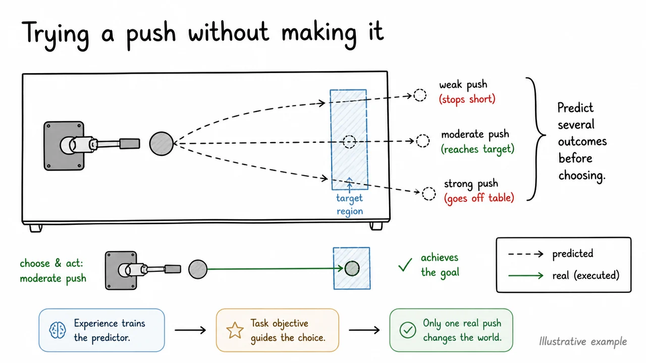
It would be useful to try a push without making it. Given the puck's current position, the robot could predict where a particular command would leave it, compare that outcome with a few alternatives, and execute the most promising one. The prediction needn't reproduce every reflection on the tabletop. It does need to preserve the difference between stopping inside the target and sliding past it. That difference is what the robot is trying to act on.
A learned world model is a way to build such a predictor from experience. The robot observes what happens when it acts, fits a model to those observations, and uses the model to answer new questions about possible actions. Here, “world” can be as small as a puck, a pusher, and the patch of table they occupy. We are trying to model the part of the environment that matters for a decision.
There are two separate pieces of work hidden in that description. Predicting that a push will move the puck ten centimeters doesn't say whether ten centimeters is desirable; the answer depends on where the target is and what else the push might do. The controller—the part of the system that selects commands—therefore needs both a model of consequences and a way to choose among them. Much of the usefulness—and many of the failures—of world models comes from how these two pieces interact.
We'll use this robot as an illustrative example throughout, simplifying it when a smaller calculation makes an idea easier to see. The aim is to understand how experience becomes a prediction, how several predictions become a plan, and how the robot can keep that plan connected to what actually happens. By the end, we will have a small planner we could implement, together with specific reasons to distrust some of its apparently good ideas.
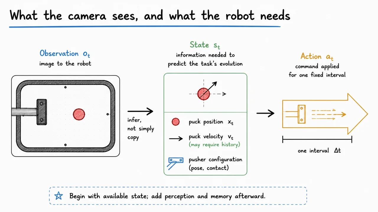
Before predicting what a push will do, we need to decide what information the prediction starts from. The robot's camera supplies an image: pixels showing the puck, the pusher, the target, and the table. We'll call that observation , where labels the current time step. An observation is what the robot receives from its sensors. It may contain details irrelevant to the task while leaving out something essential.
For example, a sharp photograph can locate the puck without telling us whether it is stationary or sliding to the right. That difference matters even if the robot does nothing. A moving puck may continue toward the table's edge; a stationary one may stay where it is. We therefore want a description that includes the information needed to predict what happens next. We will call this description the state, .
For a simplified version of our task, the state could contain the puck's position , its velocity , and the pusher's position and orientation. These quantities describe where the objects are, how the puck is moving, and whether the pusher is placed to make contact. A more detailed task might require other variables, such as a changing surface condition. Choosing a state is a modeling decision: omitted information becomes a problem when it changes the outcomes we need to predict.
The action, , describes what the robot commands over the next fixed interval. It might specify a pusher motion, including its direction and speed. This command is different from the motion the puck ultimately makes. The same motor command can have different effects depending on the starting geometry, so recording only the action would leave the predictor without enough context. The state and action belong together.
For the next few steps, suppose the relevant state is already available. Perhaps a tracking system estimates position and velocity from several camera frames. This lets us work out the prediction problem without simultaneously solving perception. We will return to how the robot infers useful information from images and history. For now, the model's input is a description of the current situation plus a command we are considering.
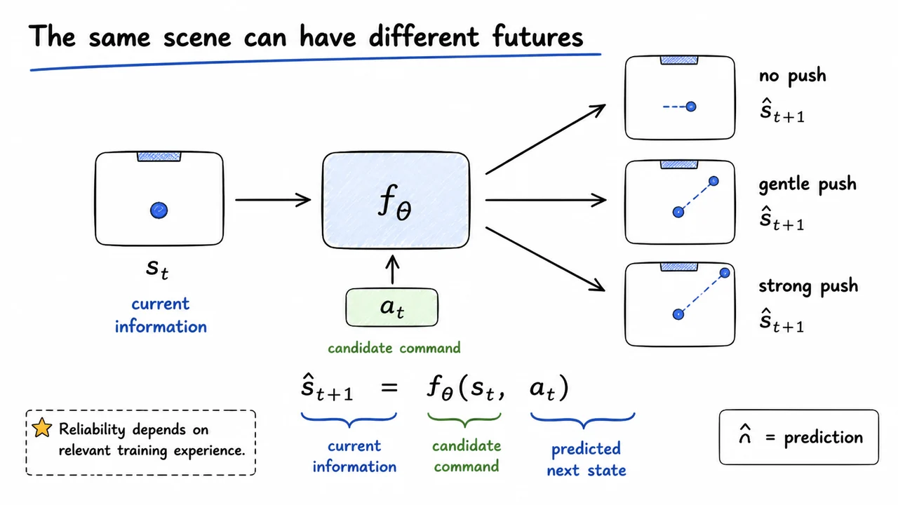
Imagine holding the starting state fixed while changing only the proposed push. With no contact, the puck might remain where it is. With a gentle push, it might stop near the target. With a stronger push, it might pass the target entirely. A predictor useful for planning must give us a way to ask about each of these possibilities. It cannot simply offer one continuation of the scene and leave the action unspecified.
The simplest version takes the current state and a proposed action, then returns a predicted next state:
Here is the learned function, and stands for its adjustable parameters. The hat on marks the output as a prediction. We haven't executed the command or measured its result. We are asking the model what it expects one interval later if we start from and apply .
This is often called an action-conditioned dynamics model. “Dynamics” refers to how the state changes over time; “action-conditioned” tells us that the proposed command is one of the inputs. For the puck, the model might combine its estimated motion with the geometry and strength of the proposed contact. It could learn that a command which moves the puck when the pusher is directly behind it does little when the pusher misses.
A model that predicts plausible video without accepting an action answers a different question. Its continuation might reflect the motions most common in its training data, but we cannot directly use that continuation to compare a gentle push with a strong one. To support this comparison, the predictor must represent how outcomes vary with the intervention we are considering. Providing an action input makes that query possible; it doesn't, by itself, make the answer reliable.
That reliability has to come from experience. If the robot has only seen gentle pushes near the center of the table, a forecast for a hard push near the edge may be little more than an extrapolation. The equation gives us a useful interface—a situation and a command go in, a predicted consequence comes out. Learning determines whether the function behind that interface has earned our confidence.
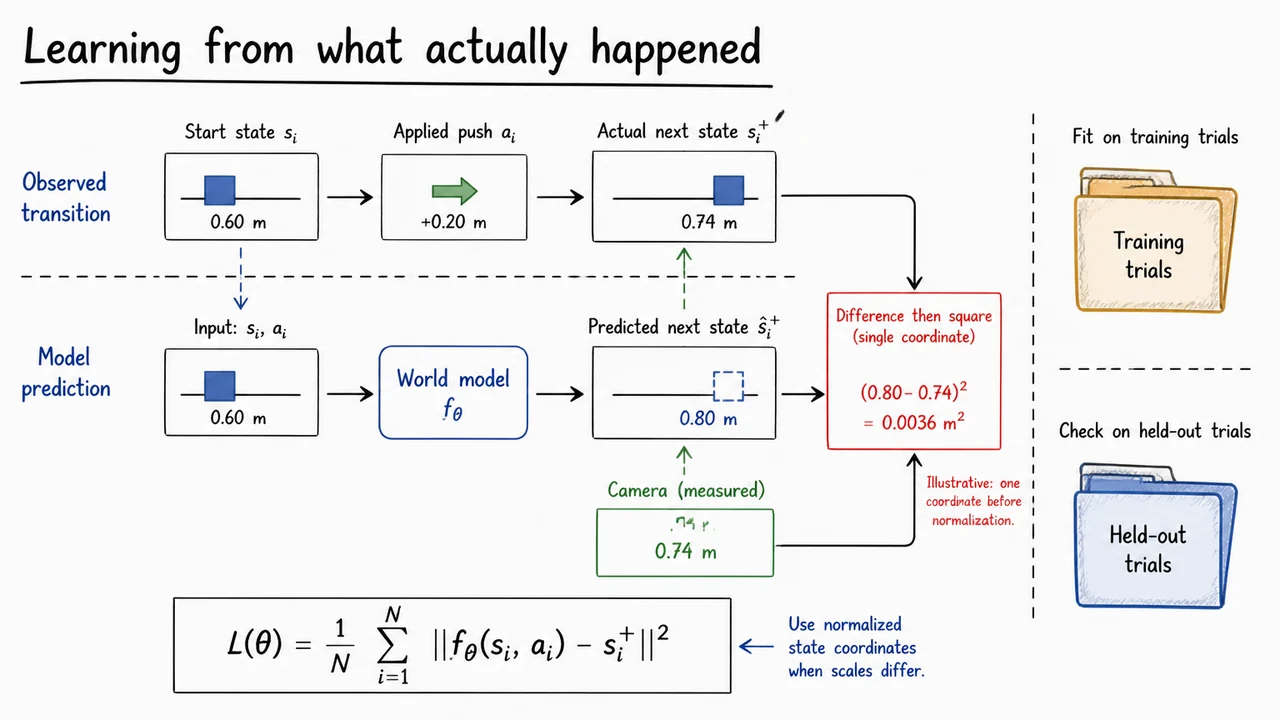
The robot can collect training examples by recording the situation before a push, the command it applied, and the situation afterward. Each example is a transition: . The index identifies an example in the dataset, and the plus sign on means “the observed next state.” It is a target obtained from experience, rather than another output of the model we are training.
For each transition, we feed the first two items into the predictor and compare its answer with the third. Suppose, in an illustrative one-dimensional position calculation, the model predicts that the puck will stop at meters, while the observed position is meters. The position error is meters. Squaring it gives square meters: a nonnegative penalty that is zero only when the two positions agree. These numbers are a toy example, not measurements from a robot experiment.
With a vector state, we can square the error in each coordinate and add those penalties. Averaging across transitions gives a simple training objective:
The expression inside the norm is the predicted state minus the observed target. The squared norm adds the squared coordinate errors; the sum combines examples; dividing by produces an average. Fitting the model means adjusting to reduce this loss. When the state mixes position, velocity, and other quantities, we should choose sensible coordinate scales or weights first. Otherwise, changing the units of one component could change what the model is rewarded for getting right.
A small training loss tells us that the model fits the examples it was shown. We still need to find out whether it predicts new trials. Holding out whole trajectories or independently collected trials is useful here: neighboring frames from the same push can be very similar, so scattering them between training and testing may make the test easier than the eventual deployment problem.
The contents of those trials matter as much as their number. Repeating a gentle push from almost the same position teaches us little about a glancing contact or a puck already moving toward the edge. Data collection therefore shapes the questions the model can answer. It also exposes cases in which our input description is missing something: if apparently identical inputs keep producing incompatible targets, fitting harder may not resolve the underlying ambiguity.
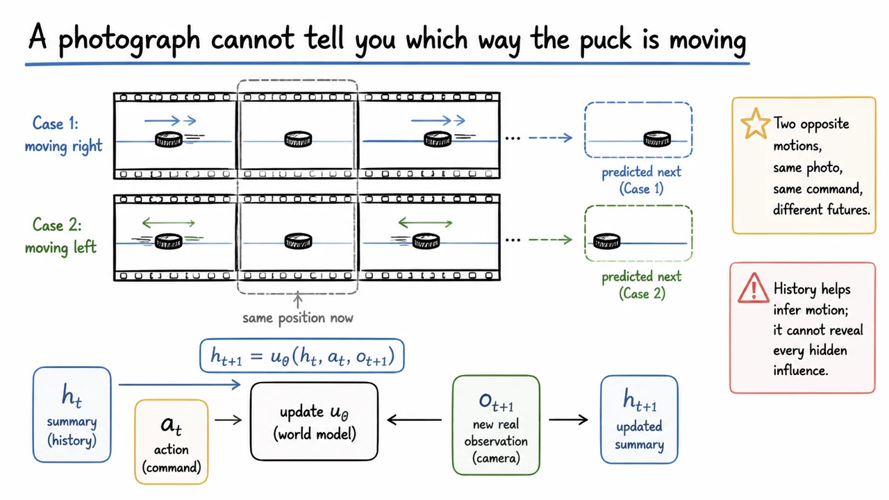
Consider two short videos of the puck. In the first, it slides from left to right; in the second, from right to left. Pause both videos when the puck reaches the same point. The current photographs may be indistinguishable, yet the puck is likely to move in opposite directions if the robot waits for another interval. A predictor given only the present position cannot know which continuation belongs to which trial.
This is a problem with the information supplied to the model. Adding more examples can teach it how common each continuation is, but cannot reveal which hidden situation produced a particular photograph. The missing clue appears in the preceding frames. Comparing positions over time allows the robot to estimate motion and give the predictor a more informative starting point. In control terminology, the camera provides a partial observation of the state.
We don't have to hand the model an ever-growing video at every step. We can maintain a compact summary of the relevant history, denoted . After executing an action and receiving a new camera observation, an update function combines the old summary with that new evidence:
The ordering matters. The robot takes , the environment responds, and the camera supplies . The summary can then be updated to reflect what happened. It might retain an estimate of velocity even when the current frame alone cannot show it. A recurrent neural network, which carries an internal memory from one time step to the next, is one way to learn such an update. An explicitly designed tracking system is another.
History does not make every state variable observable. If two surfaces look identical but have different friction, the robot may need to watch how the puck slides before it can distinguish them. Even then, noisy measurements or brief contact may leave several explanations plausible. Rather than forcing this incomplete information into a single confident forecast, the model can represent several possible outcomes and how much support it assigns to each.
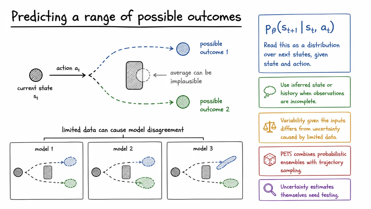
Suppose the same attempted contact sometimes sends the puck slightly left and sometimes slightly right. If we train a predictor to minimize squared error, it is rewarded for returning the average among outcomes associated with the same inputs. That average may be a useful estimate when the possibilities cluster together. It can be misleading when they form separate groups: the average of paths around opposite sides of an obstacle can run straight through the obstacle.
A probabilistic predictor describes a distribution of possible next states instead of returning only one point. We can write it as
Read the vertical bar as “given.” The model assigns probability across possible next states, given the starting state and the action. If the starting situation is only partially observed, the conditioning information should include an inferred state or a history summary. The notation is compact, but the practical question is familiar: which outcomes remain plausible after using the information available to us?
There are different reasons for a forecast to be uncertain. Some variation remains because our measurements omit details of the contact or because the process itself varies at the resolution we model. Other uncertainty reflects a lack of relevant training experience. If the robot has barely tried a particular kind of push, several models may fit its existing data while disagreeing about that push. New experience can help resolve this disagreement, although it may not eliminate variability in the physical outcome.
An ensemble makes this second situation easier to examine by training several predictors and comparing their answers. A probabilistic ensemble can also represent variation within each predictor's forecast. PETS combines uncertainty-aware dynamics models with trajectory sampling: possible model futures are sampled and propagated through the planning calculation. That is one concrete way to avoid treating a single predicted trajectory as the whole story.
For our robot, different futures may imply different choices. A push with an attractive average endpoint could still carry a substantial chance of leaving the table, while a slightly less direct push could keep plausible outcomes farther from the edge. Making that distinction requires both a distribution and an objective that pays attention to the relevant consequences. Neither a probability output nor agreement among several networks proves that the uncertainty estimate is trustworthy. Models trained on similar data can share the same blind spot, so their forecasts need to be checked against outcomes.
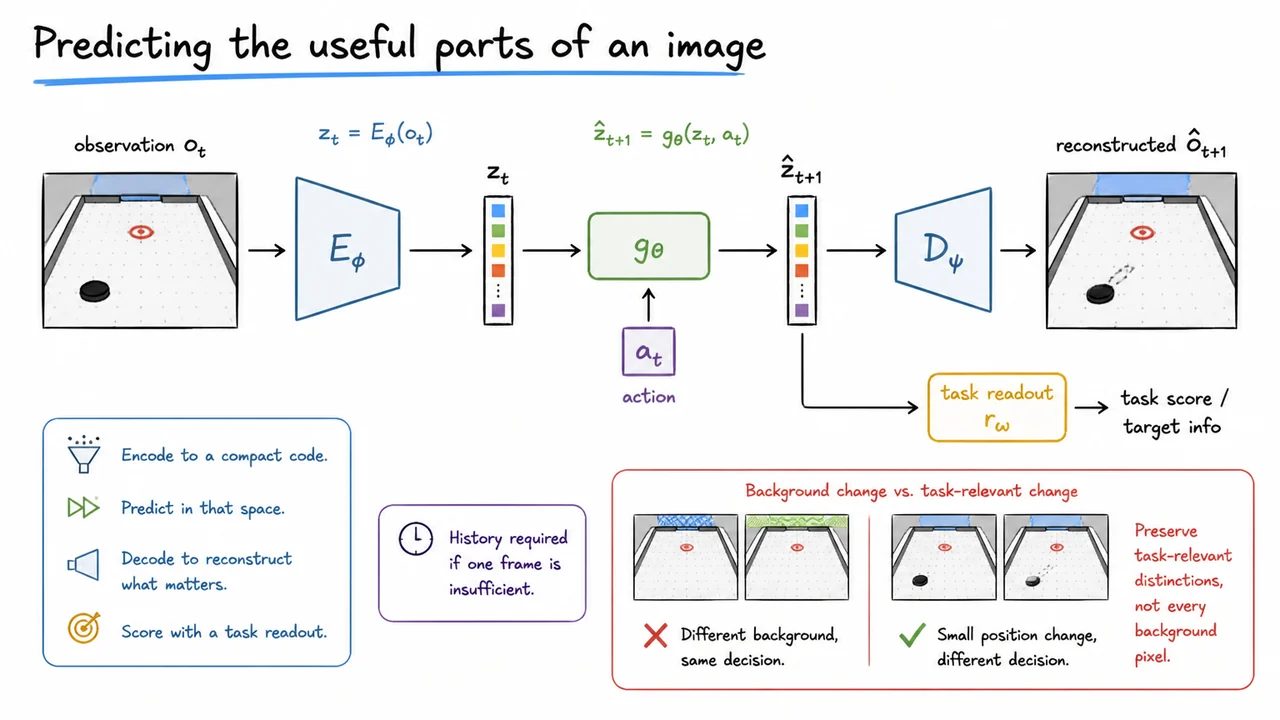
Our equations have treated the state as a convenient vector of relevant quantities. A camera, however, gives the robot an image. Predicting the next image pixel by pixel is possible, but it asks the model to account for a great deal of appearance: the table's texture, lighting, shadows, and the puck's position. A small position error may matter more for the next action than a large error in the background, even when a pixel-based loss says otherwise.
An encoder offers a way to work with a more compact description. It maps the observation into a vector, or latent code:
The encoder has parameters , learned from data. Its output can be much smaller than the image. The coordinates need not correspond neatly to physical quantities such as position and velocity; the network may distribute useful information across many entries. “Latent” simply tells us that this is an internal representation, rather than the raw observation.
In a simplified setting where one code contains enough information, we can learn a predictor for the next code:
This has the same basic structure as our state predictor. The difference is that the model now predicts in a learned representation. If one image leaves motion ambiguous, compressing that image does not recover the missing history. We still need temporal information, whether it is built into the representation or maintained by a separate state estimator.
A decoder, , with its own learned parameters , can map a code back into an image. Reconstructing the current observation gives one way to train the representation, and decoding predicted codes lets us inspect what the model expects to see. But a controller doesn't necessarily need to render each imagined future. It needs a way to assess what those codes imply for the task—for example, a readout that estimates the puck's position or its distance from the target.
That readout is a substantive part of the design. Two nearby vectors in an arbitrary learned space need not mean that the puck is physically near the target. The training objective has to encourage useful distinctions, and the decision procedure has to interpret them appropriately. We have gained a compact space in which to predict; we have also taken responsibility for what that space preserves.
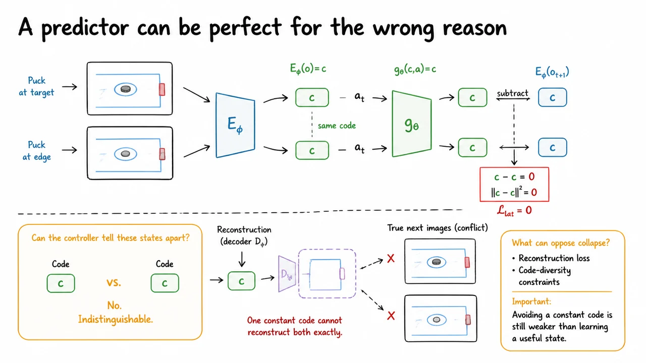
There is a tempting way to train the encoder and predictor together. Encode the current image, predict its successor code under the recorded action, and compare that prediction with the encoding of the next real image. If the codes match, reward the system. This seems to ask exactly what we want: learn a representation in which the future is predictable from the present and the action.
For a single transition, the squared-error objective is
The difficulty is that the encoder helps produce both sides of the comparison. It can change the prediction problem while the predictor learns to solve it. Suppose the encoder maps every possible image to the same vector . The puck inside the target, the puck at the table's edge, and an empty table now all receive identical codes. If the predictor also returns for every action, then
Every transition earns a perfect score. Yet the controller has lost the distinction between a situation in which it should stop and one in which it might need to intervene. This failure is called representation collapse. The model has satisfied the written objective by making its targets uninformative. The problem is already visible in this simple calculation; it does not depend on a difficult optimization failure.
Additional training requirements can make the constant solution unattractive. If a decoder must reconstruct distinct input images from their codes, a single constant code cannot provide the information needed to reconstruct all of them exactly. Other approaches constrain the representation so that its outputs retain variation across examples. The details matter, because they determine which alternatives to collapse the system can learn.
Even a varied code is only a beginning. A representation could change with the tabletop texture while failing to distinguish whether the puck is moving toward the target or away from it. Preventing a constant output removes one obvious failure, but usefulness still depends on retaining information that supports prediction and action. We should therefore inspect what the learned representation makes possible, rather than treating a low latent prediction loss as evidence that the robot understands its situation.
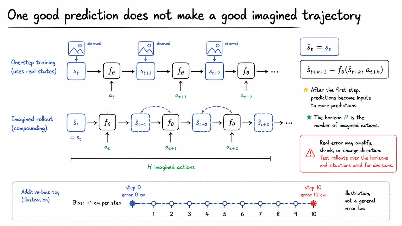
Once we have a useful one-step predictor, we can ask it about a sequence of pushes. Predict the state after the first command, feed that predicted state back into the model with the second command, and continue. This repeated simulation is a rollout. The number of actions we simulate is the planning horizon, . A horizon of five means that each candidate plan looks five action intervals into the future. We'll use state notation again for clarity; the same chaining of predictions applies in a latent space.
Starting at the current state, the calculation is
The index counts how far ahead we have imagined. On the first step, the model receives the state available from the real environment. On later steps, it receives its own predictions. This change of input is easy to overlook. A model tested only by predicting one observed frame from another has not yet been tested in the conditions created by a long rollout.
A simple toy calculation shows why the difference matters. Suppose the true one-dimensional motion adds the commanded displacement at each step, while our model adds that displacement plus an extra centimeter. The first predicted position is one centimeter too far forward. The next prediction starts from that already shifted position and adds another centimeter of bias. After ten steps, the predicted endpoint is ten centimeters ahead of the true one, even though every isolated one-step error looked small.
Real errors do not always follow this linear pattern. A mistake in position can change whether the predicted pusher makes contact, producing a much larger change in the next state. Depending on the system's dynamics, some differences may shrink instead. The useful lesson is to examine how the model's errors behave when predictions become inputs, over the horizons and situations that the controller will actually use.
Longer rollouts can reveal consequences that a short forecast misses, such as a push that first moves the puck away from the target to improve a later contact. They also give the model more opportunities to drift. Choosing a horizon therefore involves a practical tradeoff between seeing far enough to choose sensibly and relying on predictions that remain informative. To make that tradeoff concrete, we need to specify how a predicted trajectory earns a good or bad score.
A trajectory is useful to the controller only if it can tell whether that trajectory serves the task. For our puck, ending close to the target is desirable, but so is avoiding unnecessarily forceful commands or dangerous intermediate states. We can express these preferences as costs: smaller numbers represent outcomes we prefer. This choice belongs to the task designer. A predictor trained to forecast motion does not automatically know what the robot is supposed to accomplish.
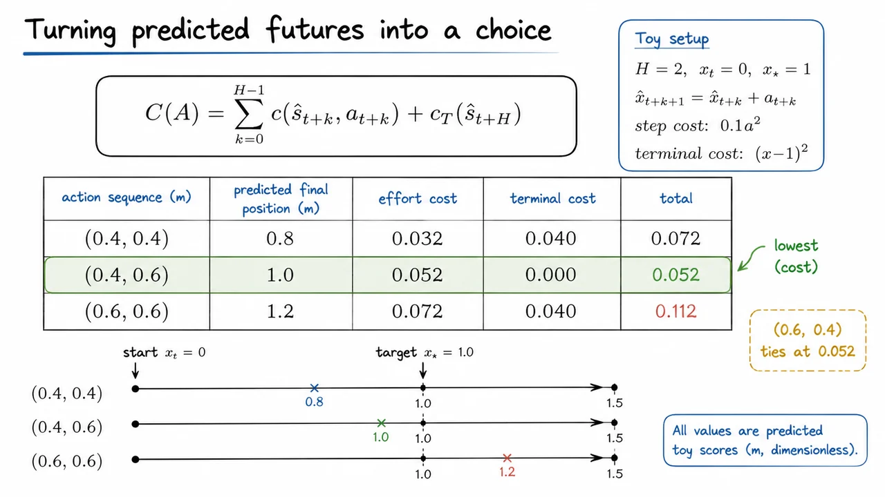
Let be a candidate sequence of actions. For a first planner, we'll use point predictions and explicit state variables. A per-step cost scores each state and action, while a terminal cost scores the state at the end of the horizon. Their total is
The sum charges for the actions and their starting states. The final term evaluates where the resulting sequence leaves us. Here is a cost function, unrelated to the constant vector used in the collapse example. By keeping intermediate and terminal costs separate, we can describe both how we want the robot to move and where we want it to finish.
For an arithmetic example, simplify the puck to one-dimensional position. It starts at , the target is at , and each action commands a displacement of either or meters. Assume the toy model predicts that displacement exactly: each next position is the previous position plus the action. Use two actions, a step cost of , and a terminal cost of , with distances entered as their numerical values in meters. These are illustrative dimensionless scores, not a physical energy calculation.
Consider three candidate sequences:
| Sequence | Predicted endpoint | Step costs combined | Terminal cost | Total |
|---|---|---|---|---|
| m | ||||
| m | ||||
| m |
For the mixed sequence, the step costs are . Its endpoint is exactly the target, so it incurs no terminal penalty. It beats the two gentler pushes because their lower effort cost doesn't compensate for stopping short. Reversing the mixed sequence gives the same score in this simple model, though order could matter in a system with momentum, obstacles, or contact.
We have now converted a prediction into a choice. The qualification is visible in the calculation: we selected the lowest predicted cost among the candidates considered, using a deliberately simplified model and objective. A richer controller could evaluate sampled uncertain futures or add constraints. Even this small version is enough to show how a task preference and a learned transition model work together.
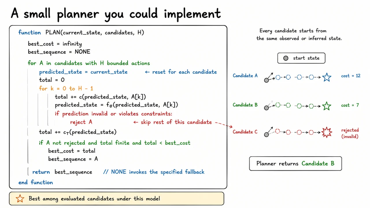
The calculation in the table can be turned into a planner with two loops. The outer loop considers candidate action sequences. The inner loop simulates one candidate, accumulating its cost as it goes. Each candidate must start from the same current state; otherwise, we would be comparing plans for different situations. The model's parameters stay fixed during this search. We are choosing actions with the model, rather than training it.
The pseudocode below assumes a positive horizon and that we have supplied the dynamics function, the two cost functions, and any constraints that candidates must satisfy. “Invalid” includes a prediction that fails numerically, and “feasible” means that the predicted state meets the constraints we chose. Neither check establishes that a real-world action is safe when the model itself is wrong.
function PLAN(current_state, candidates, H)
    best_cost = infinity
    best_sequence = NONE

    for A in candidates:
        if length(A) != H or actions_out_of_bounds(A):
            continue

        predicted_state = copy(current_state)
        total = 0
        rejected = false

        for k = 0 to H - 1:
            total = total + c(predicted_state, A[k])
            predicted_state = f_theta(predicted_state, A[k])
            if invalid(predicted_state) or not feasible(predicted_state):
                rejected = true
                break

        if rejected:
            continue

        total = total + c_T(predicted_state)
        if finite(total) and total < best_cost:
            best_cost = total
            best_sequence = A

    return best_sequence
end function
Notice where the costs enter. We add the step cost before advancing the predicted state, matching the convention in the equation. After the last transition, we add the terminal cost exactly once. A candidate rejected partway through is skipped entirely. If all candidates are rejected, the function returns NONE; the caller must then follow an explicit fallback procedure instead of pretending that a plan was found.
For the two-action toy problem, we can enumerate all four possible sequences. With many continuous actions, enumeration soon becomes impractical, so a simple alternative is to sample a finite collection of bounded sequences. The same scoring loop still works. More candidates give the search more opportunities to find a good predicted plan, but do not improve the predictor's knowledge of the environment. We will need that distinction when examining what happens after the planner starts making real choices.
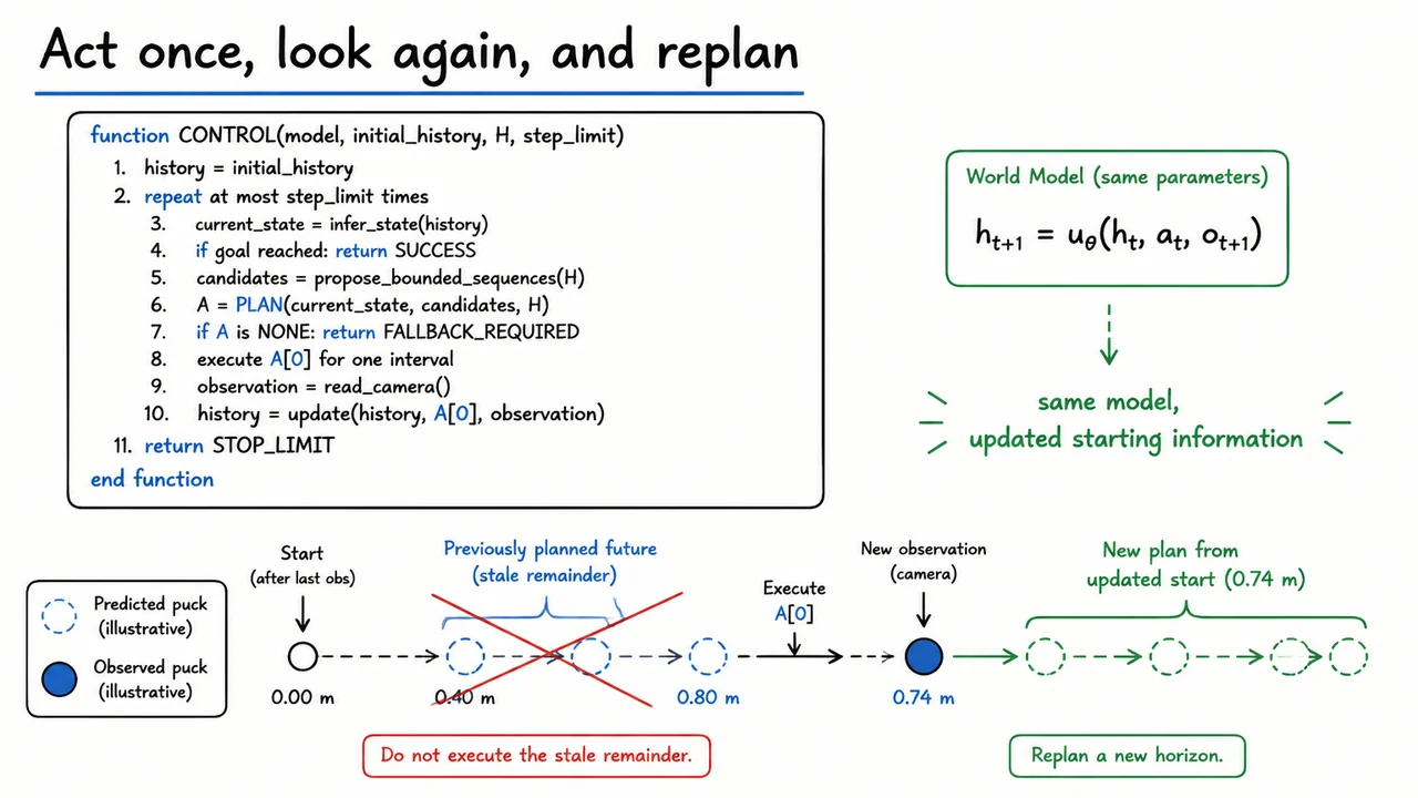
Suppose the planner has selected a five-push sequence. It might seem natural to send all five commands to the robot. But the second command was evaluated from the model's prediction of where the first push would leave the puck. If the first contact goes differently, the remaining plan starts to describe a situation the robot is no longer in. We can use the camera to update that starting information before committing to another push.
The resulting procedure is called receding-horizon control, or model predictive control. Plan several steps ahead, execute only the first action, observe the result, and plan a fresh horizon from the updated state estimate. The unused actions helped us judge the first action's consequences. They are provisional; the robot doesn't owe them execution once new evidence arrives.
In our earlier numerical example, a model predicted a puck position of meters while the observed position was meters. Replanning uses the observation to update the state estimate instead of continuing from the old predicted position. This does not automatically change the dynamics model's parameters. The next prediction can still be wrong for the same reason as the previous one. What changes immediately is the information from which the next plan begins.
Using the history update introduced earlier, the surrounding control loop can be written as follows. The history begins with the available observations, and the model, costs, constraints, and candidate generator are supplied by the application.
function CONTROL(initial_history, H, step_limit)
    history = initial_history

    repeat at most step_limit times:
        current_state = infer_state(history)
        if goal_reached(current_state):
            return SUCCESS

        candidates = propose_bounded_sequences(H)
        A = PLAN(current_state, candidates, H)
        if A is NONE:
            return FALLBACK_REQUIRED

        execute A[0] for one interval
        observation = read_camera()
        history = update(history, A[0], observation)

    if goal_reached(infer_state(history)):
        return SUCCESS
    return STOP_LIMIT
end function
The final goal check uses the observation after the last permitted action, so reaching the target on that action still counts as success.
Feedback helps because each new plan can incorporate evidence that was unavailable when the preceding plan was made. It doesn't remove every source of failure. A noisy camera can produce a poor state estimate; a short horizon can miss a later consequence; and observing a puck after it has fallen off the table cannot undo the action that sent it there. The value of replanning lies in making subsequent decisions from fresher information, within the limits of sensing, prediction, and the time available to react.
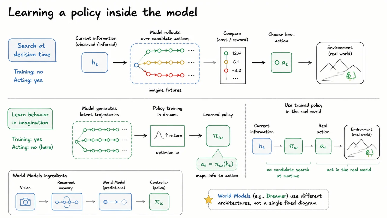
Searching through candidate sequences every time the robot moves is one way to use a world model. Another is to use imagined experience to train a decision rule in advance. Such a rule is called a policy. Given the information available now, it produces an action. With representing that information and denoting the policy's learned parameters, we can write
For the puck, a policy might learn to choose a pusher motion from the estimated position, motion, and target relationship. Instead of evaluating a fresh collection of sequences for every real push, it applies a function whose parameters have already been adjusted through training. The model can still be involved in estimating the current situation; using a policy does not mean the robot stops processing observations or maintaining memory.
Imagined rollouts provide a place to improve that policy. Starting from a suitable state, the policy proposes an action, the world model predicts what follows, and the policy proposes another action from the imagined situation. The resulting trajectory can be scored against the task. A learning procedure adjusts the policy to favor behavior with better predicted outcomes. In reinforcement learning, it is common to express this score as reward, with larger values preferred, rather than as a cost to minimize.
This broad distinction helps separate methods that are sometimes grouped together. In the original World Models work, a vision component compresses the observation and a recurrent memory component models temporal structure. A small controller uses the current visual code and memory state to choose an action. The predicted next visual code is not fed directly into that controller. The work also explores training a controller inside a learned dream environment and transferring it to the actual environment.
Dreamer develops behavior learning through imagined trajectories in a learned latent state space. It uses learned state values to estimate future reward and derivatives, or gradients, to guide changes in behavior through imagined trajectories. Those derivatives indicate how small changes in the policy affect the predicted reward. The relevant connection to our example is that the model supplies experience for improving a reusable policy, rather than merely supplying a fresh list of candidate plans to rank at each physical decision.
Both routes still depend on the quality of the experience the model supplies. Online search can favor an action because its predicted trajectory looks attractive. A policy trained in imagination can learn to seek the same kind of attractive trajectory repeatedly. In either case, improving the decision-maker against the model can expose weaknesses that were easy to miss when the model was evaluated only as a predictor.
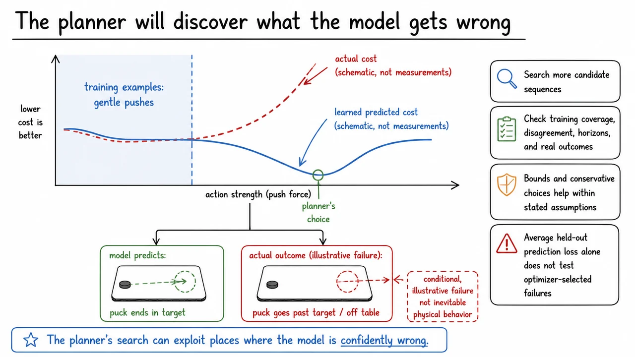
Suppose most of the robot's training data contains gentle pushes. Within that range, the learned model predicts the puck's motion reasonably well. Outside it, the model happens to predict that a much stronger command will produce a long, controlled slide ending near the target. The real puck might overshoot or respond unpredictably, but those outcomes are absent from the calculation. To the planner, the unsupported prediction can look like an excellent opportunity.
The planner has no reason to avoid that opportunity unless its objective or constraints give it one. Its job is to find a low predicted cost. By searching many possibilities, it may concentrate precisely on the region where the model is most optimistic. An error that affected only a small fraction of randomly chosen test actions can therefore become a frequent error under the controller's own choices. The distribution of actions has changed because we started optimizing.
This explains why increasing the search budget is not always a remedy for poor real-world performance. More candidates improve coverage of the action space we are searching. They do not provide new observations of what those actions actually do. If the additional candidates include more opportunities to exploit a bad prediction, a better search can find plans that look better in the model while working worse on the table.
We can respond at several points in the loop. Action bounds can keep candidate commands within a range supported by experience. Collecting data in relevant new situations can improve the model there. Disagreement among predictors can flag some uncertain candidates, and shorter horizons can reduce reliance on distant forecasts. Each intervention addresses a particular source of trouble; none makes an untested prediction correct by definition. Shared model errors and irreversible actions remain possible.
The test should therefore include the choices the controller is actually making. If a robot repeatedly selects a kind of push that fails despite receiving a low predicted cost, averaging that error together with thousands of easy predictions hides the important fact. The model is wrong where its answer changes behavior. Understanding that failure requires looking at prediction, selection, and real outcome as one connected process.
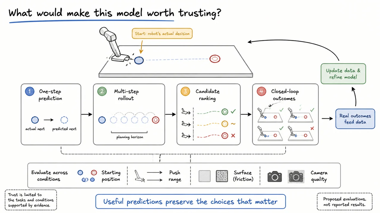
Return to the robot waiting beside the puck. It now has a procedure for considering a push before making it: infer the current situation, imagine candidate consequences, compare their costs, and take an action. The remaining question is practical. What evidence would convince us that this procedure helps, under the conditions in which we intend to use it?
We could begin with held-out trials and check the state components that matter for the task. Does the model predict the puck's position and motion after a push? Does it distinguish contact from a miss? Keeping the evaluation separate from training helps us see whether the model has learned more than the examples it already knows. Testing several starting positions and command strengths also makes the limits of that evidence more visible than a single average score.
Next, we would evaluate complete rollouts over the proposed planning horizon. A model may make accurate one-step predictions while drifting too far to compare five-step plans. We should then examine whether its candidate rankings survive contact with the real system: when it prefers one sequence to another, does that preference agree with outcomes from comparable starting conditions? Such comparisons require controlled trials or appropriate repeated measurements, since executing one sequence changes the state for the next. These are proposed evaluations for our example, not reported experimental results.
Finally, we would test the closed loop itself: repeated observation, planning, action, and feedback. Record both task completion and the ways attempts fail, while varying the conditions we expect the robot to encounter. A change in surface friction, a poor camera observation, or a start near the edge can reveal a limitation that ordinary trials conceal. The relevant question is how the whole procedure behaves when its predictions influence which data it encounters next.
A beautiful predicted video might pass none of these tests. A much plainer internal representation could pass them if it preserves the distinctions needed to choose well. The model's value comes from making useful consequences available before the robot acts: this push is likely to stop short, that one depends on a contact we cannot estimate reliably, and another is worth trying from the position we have actually observed.
The robot still has to make a real push. What it gains is a better basis for choosing that push, and a way to use the result when choosing the next one.